Research Progress on Spatiotemporal Interpolation Methods for Meteorological Elements

Abstract

With the development of mathematical statistics, people have developed the spatiotemporal interpolation methods based on the spatial interpolation method or the temporal interpolation method. These methods fully consider the comprehensive effects of time series changes and spatial distribution to better handle complicated and changeable meteorological element data. This article systematically reviews the current research progress of spatiotemporal interpolation methods for spatiotemporal sampling data of meteorological origin. Spatiotemporal interpolation methods of meteorological elements are classified into three categories: spatiotemporal geostatistical interpolation methods, spatiotemporal deterministic interpolation methods, and spatiotemporal mixed interpolation methods. This article summarizes the theoretical concept and practical application of the spatiotemporal interpolation methods of meteorological elements, analyzes the advantages and disadvantages of using spatiotemporal interpolation methods for estimating or forecasting meteorological elements, combined through some measures and their application to explain the accuracy of the spatiotemporal interpolation methods; and discusses the problems and challenges of spatiotemporal interpolation. Finally, the future research focus of spatiotemporal interpolation methods is proposed. This article provides a valuable method reference for estimating or predicting meteorological elements such as precipitation in unsampled points.

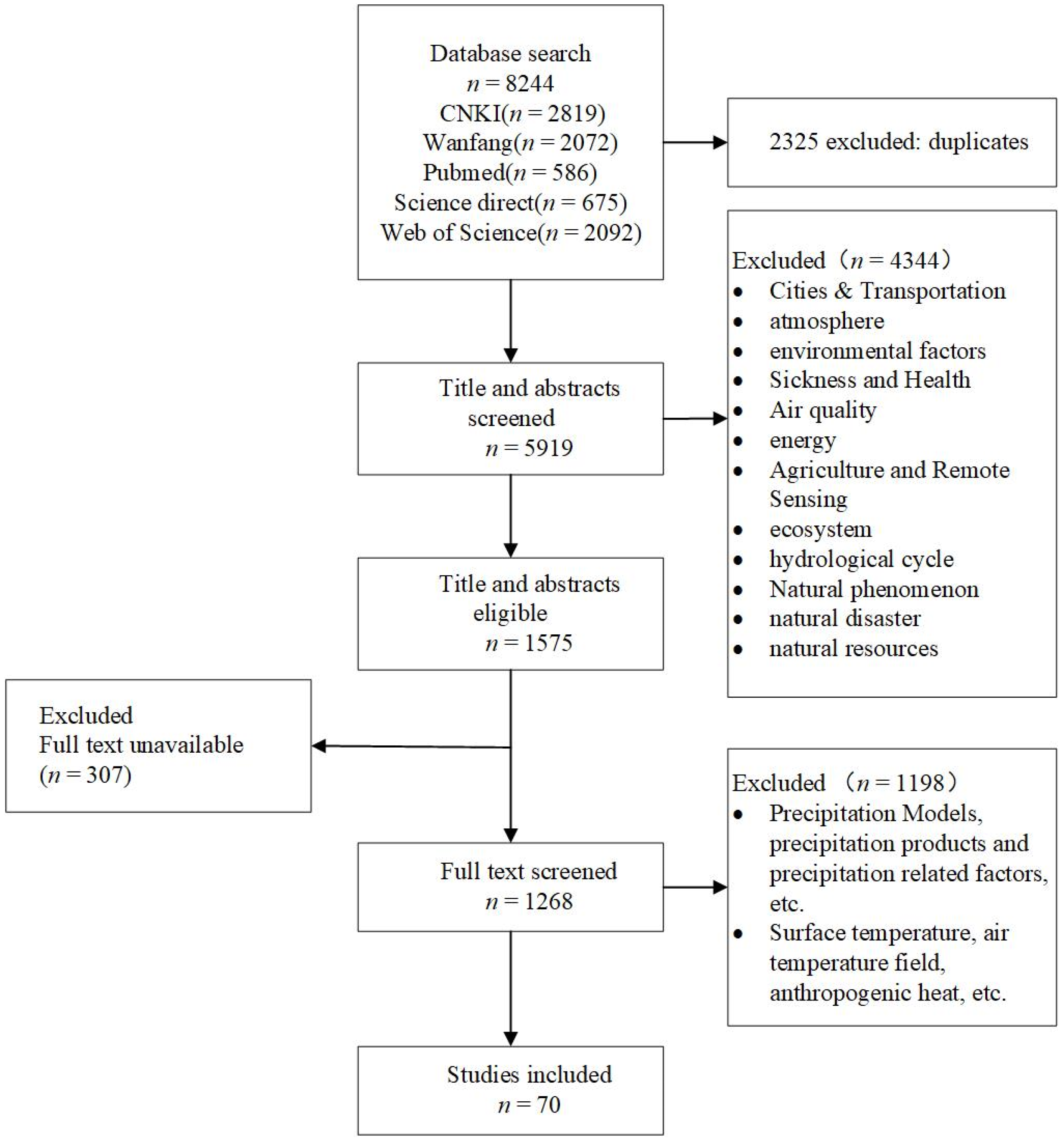
1. Introduction

The scientific community is becoming more and more concerned with the topic of global climate change and its repercussions [1,2]. Conventional meteorological element data mostly depend on station observation [3]. However, since there are not sufficient meteorological observation stations as there should be in light of topographical factors, economic factors, and technical limitations, meteorological element data are typically unavailable in many locations, and this has an impact on people’s judgment and decision-making.

To address these issues, researchers typically use and mine the temporal or spatial autocorrelation of meteorological elements, as well as the temporal or spatial correlation between meteorological elements and auxiliary variables based on particular mathematical frameworks and generate the raster data that are continuous and cover the whole region by predicting the whole study area through the data of the sample points in the study area [4]. For time series of climatic elements, common interpolation techniques include the autoregressive model, moving average model, generalized summation model, etc. Nevertheless, these approaches severely lack the ability to characterize the geographical distribution of meteorological parameters and neglect their spatial structure and continuity [5]. Spatial interpolation is typically categorized as either deterministic or geostatistical [6]. The geostatistical interpolation methods primarily comprise kriging interpolation [1] and stochastic simulation [7]. The deterministic spatial interpolation comprises the Tyson polygon, inverse distance weight method, trend surface, multiple regression method [8], polynomial interpolation, and spline function. There is no definitive standard model for the spatial interpolation method of meteorological factors because topography and station distribution vary so much [9]. This method only considers the spatial relationship between sampled and unsampled points in the study area, or the spatial relationship between meteorological observation stations and the points to be estimated; it does not consider the temporal correlation of the meteorological factors, meaning that historical data on meteorological factors cannot be used to judge meteorological factors in the present or the future.

Meteorological element observations, such as temperature, humidity, and precipitation, are examples of typical spatiotemporal data that exhibit high temporal and spatial correlations. Researchers currently often consider space and time separately when interpolating and evaluating meteorological element data [10], or reduce spatiotemporal data to a set of spatial data for spatial interpolation [11]. It is not possible to gather meteorological data for the points that need to be approximated with a greater level of accuracy by using any of the methods that deal with space and time independently. Consequently, in order to produce a dataset that covers both space and time, a spatiotemporal interpolation technique that combines temporal and spatial information is required [12]. The spatiotemporal interpolation method is primarily used with spatiotemporal sampling data, which not only solves the problem of statistical difficulties due to the incomplete time series of meteorological data but also solves the decrease in interpolation accuracy caused by fewer observation stations [13], and it is of great significance to the spatiotemporal mining and modeling of meteorological data.

Significant advancements have been made in the study of interpolation techniques for meteorological components like temperature, humidity, and precipitation, among others, thanks to the growth of meteorology and statistics. A systematic review of the techniques used for the spatiotemporal interpolation of the synthesized meteorological element data is lacking. Currently, researchers primarily examine the spatial interpolation methods of meteorological elements and compare the interpolation accuracies [6,9,14,15,16,17,18]. A few researchers have also looked into the methods of interpolation, reconstruction, and prediction of heterogeneous sparsely distributed spatiotemporal data. This research conducts a thorough analysis of the current spatiotemporal interpolation models considering this. It reviews and organizes the indexes of evaluating the spatiotemporal interpolation methods; looks ahead to the direction of future research development; and summarizes the spatiotemporal interpolation methods of precipitation and other meteorological elements from the three aspects of spatiotemporal geostatistical interpolation, spatiotemporal deterministic interpolation, and spatiotemporal hybrid interpolation. For the purpose of calculating or forecasting meteorological factors like precipitation, this paper offers helpful methodological references.

2. Methodology

The purpose of the search strategy in this paper is to determine the methodology for spatiotemporal estimation or prediction of meteorological element data at the point to be estimated. Three English databases, PubMed, Science direct, and Web of science; and two Chinese databases, CNKI and Wanfang database, were searched without time constraints. The core content of the search was meteorological factors and spatiotemporal interpolation, and the search expression was TI = (“spatiotemporal”) AND AB = (“interpolation” + “estimation” + “Forecast”) AND AB = (“Meteorology” + “Climate” + “Weather” + “humidity” + “temperature” + “precipitation” + “rainfall”); due to the differences between the Chinese and English interpretations, the search terms were changed accordingly. Last searched on 6 June 2023.

Following the removal of duplicate articles, the following criteria were used to screen the literature for this study: (1) based on the article titles and abstracts, the literature in subjects unrelated to describing meteorological elements was excluded; (2) the literature written by authors who were not able to access the original article was not included; (3) full text based on the topic of this study excludes the literature investigating the features of spatial and temporal changes in meteorological elements, correlates of meteorological elements, and spatial and temporal models in other domains; and (4) the literature on non-spatiotemporal sampling data was excluded based on data types, e.g., models using surface data or gridded data for spatiotemporal estimation. The process of the literature screening is shown in Figure 1.

Research topic, research area, research population, data source, data processing, sample size (representative stations), study unit/spatial scale, study timeframe, timescale/temporal resolution, and study methodology (temporal variability (trend)/interpolation, spatial variability/interpolation, spatial–temporal variability/interpolation, and accuracy tests) were all taken from the literature that was included in the study.

3. Results

3.1. Characteristics of the Study

A total of 70 documents were eventually included in this study after 8244 documents were retrieved from five Chinese and English databases. Duplicates were eliminated, and the articles were filtered based on their title, abstract, and full text. It is essential to represent the link between spatiotemporal variables to solve the spatiotemporal interpolation problem, which involves considering both spatial and temporal correlation simultaneously. Remember that the spatiotemporal interpolation method is a way to interpolate spatiotemporal sampling data. In other words, it is a way to interpolate the observation data from the study area’s observation stations and ultimately obtain full-coverage continuous raster values. The spatiotemporal interpolation techniques that are now in use are divided into three categories in this paper: spatiotemporal geostatistical interpolation, spatiotemporal deterministic interpolation, and spatiotemporal mixed interpolation.

3.2. Spatiotemporal Geostatistical Interpolation

Based on the idea of regionalized variables with a spatial distribution and the variational function, geostatistics is the science of examining natural occurrences that are both random and organized in their spatial distribution [19]. By considering the temporal element as an extra dimension that is strongly related to the spatial factor, spatiotemporal geostatistics solves the challenge of predicting the valuation of regionalized variables in the spatiotemporal domain and characterizes the correlation of those variables [20]; compared to geostatistical interpolation, more precise estimations and forecasts can be made [21]. The spatiotemporal geostatistical techniques which are most frequently employed are spatiotemporal kriging (STKriging) [22] and Bayesian Maximum Entropy (BME) [23]. These spatiotemporal statistical models efficiently represent the spatiotemporal dependence and non-stationarity of the interaction between spatiotemporal variables and employ statistical inference to illustrate the relationship between variables [24].

3.2.1. Spatiotemporal Variability Function

In environmental science and geophysics, a statistical analysis of dynamic processes depends strongly on spatiotemporal variability [25]. The degree of proximity of environmental variables on the spatiotemporal domain is objectively described by the spatiotemporal variability function [20]. In this study, we denote ${\mathbb{R}}^2$ as the two-dimensional Euclidean space, where variables are defined and interpolated. Assume that $Z(s,t)$ is a variable on the time–space of $\left\{\right(s,t\left)\right|s\in {\mathbb{R}}^2,t\in \mathbb{R}\}$ and satisfies second-order smoothness, and its covariance function and variability function are as follows:

$$C(h_s,h_t)=Cov\left(Z\right(s+h_s,t+h_t)-Z(s,t\left)\right)$$

(1)

$$\frac{1}{2}E{\left(Z(s+h_s,t+h_t)-Z(s,t)\right)}^2={\sigma }^2-C(h_s,h_t)$$

(2)

where $h_s,h_t$, respectively, represent spatial and time interval variables; and ${\sigma }^2$ is the variance of $Z(s,t)$. If the spatiotemporal variability of two variables is to be investigated, a spatiotemporal covariance function is constructed to characterize the spatiotemporal continuity of the crossover between the two variables:

$${\gamma }_{12}(h_s,h_t)=\frac{1}{2}E\left\{\left[Z_1(s+h_s,t+h_t)-Z_1(s,t)\right]\left[Z_2(s+h_s,t+h_t)-Z_2(s,t)\right]\right\}$$

(3)

$Z_1(s,t)$ and $Z_2(s,t)$ are two different variables on the space–time point, $(s,t)$. An important prerequisite for the construction of the spatiotemporal variability function is the assumption that the spatiotemporal variables satisfy second-order smoothness. Treating the meteorological factor data as a time series on a spatial observatory, the time-series decomposition of the meteorological factor data is given as follows:

$$Z(s,t)=S(s,t)+T(s,t)+R(s,t)$$

(4)

$S(s,t)$ is a seasonal term, $T(s,t)$ is a trend term, and $R(s,t)$ is a random term. To keep overall trend changes and data continuity, the seasonal or time trend item is eliminated from the time series.

There are two kinds of spatiotemporal covariance functions: separable models and non-separable models. The separable model is a composite treatment of pure temporal and spatial covariance functions by multiplication or linear combination, such as the spatiotemporal product model, which is simpler to construct but cannot portray the spatiotemporal interaction part of spatiotemporal regionalized variables [26]. The non-separable model successfully shows the correlation of variables in time and space; the process of modeling is difficult [27]. There are two widely used non-separable models: the spatiotemporal product–sum model and the spatiotemporal summation model [23,28,29].

The spatiotemporal variational function model can be optimized and improved in certain ways to effectively increase the accuracy of the interpolation. As an example, the combination of STKriging and the elastic net algorithm solves the problem that the spatiotemporal variability function matrix in the process of solving the weight coefficients in the STKriging algorithm is unable to invert the condition number directly because of its pathological characteristics. The accuracy of the method on the interpolation of meteorological and spatiotemporal data has been verified through the use of the measured air temperature data and AQI data with the spatial kriging, ESCP, STARMA, and STESN algorithms [30].

3.2.2. Spatiotemporal Kriging

The estimate for a spatiotemporal point is a weighting of the observed values of the meteorological elements surrounding that spatiotemporal location in spatiotemporal kriging, a spatiotemporal extension of the kriging method [28]. Spatiotemporal ordinary kriging (STOK), Spatiotemporal CoKriging (STCK), Spatiotemporal Universal Kriging (STUK), Spatiotemporal Regression Kriging (STRK), Modified Median Polish Kriging (MMPK), and Fixed Rank Filtering (FRF) are spatiotemporal kriging techniques that are frequently used in meteorological research. The ordinary kriging interpolation formula for spatiotemporal data is as follows:

$$Z(s,t)=\sum _{i=1}^N{\lambda }_{i}Z(s_i,t_i)$$

(5)

where $Z(s,t)$ is an estimate of the meteorological element at point $(s,t)$, $Z(s_i,t_i)$ is an observation of the meteorological element at space–time point $(s_i,t_i)(i=1,\dots ,N)$, and ${\lambda }_i$ is a kriging weighting coefficient [31].

STCK is an additional covariate to STOK with the following interpolation formula:

$$Z_{CK}(s,t)=\sum _{i=1}^{N_1}{\alpha }_{i}Z(s_i,t_i)+\sum _{j=1}^{N_2}{\beta }_{j}V(s_j,t_j)$$

(6)

where $Z_{CK}(s,t)$ is the estimated value of the main variable at point $(s,t)$; $Z(s_i,t_i)$ is the observed value of the main variable at station $(s_i,t_i)(i=1,\dots ,N_1)$; ${\alpha }_i$ is a set of weight coefficients assigned to the main variable at each station; $V(s_j,t_j)$ is the observed value of the covariate at station $(s_j,t_j)(j=1,\dots ,N_2)$; ${\beta }_j$ is a set of weight coefficients assigned to the covariate at each station; $N_1$ and $N_2$ are the number of stations used for interpolation for the main variable and covariate, respectively $N_1\le N_2$. STCK can be calculated in R using the gstat and space–time packages [32]. STCK with monthly mean precipitation from 54 stations in Xinjiang Province, China, as the main variable and monthly mean air humidity at the same time in the same area as the auxiliary variable is more accurate than STOK interpolation [23,30].

Spatiotemporal Universal Kriging (STUK), which is linear and non-stationary, is also useful for estimating or predicting meteorological data at a given moment in time. Spatiotemporal Universal Kriging (STUK) measures the spatial distribution characteristics of meteorological factors based on the trend at each station and the residual variance of the observed values of meteorological factors at a given moment from the trend [5]. STUK was applied to reconstructed meteorological records from 150 observation stations in 10 provinces and cities in China for one year and compared with linear interpolation, standard ratio (normal ratio, NR), and OK, considering the effect of elevation and altitude, and it was found to have the highest interpolation accuracy. Meanwhile, STUK is suitable for small watersheds with no precipitation observatory distribution and can be used as a method for watershed precipitation calculation [33].

The combination of spatiotemporal kriging and regression modeling is called Spatiotemporal Regression Kriging (STRK). The method can be used not only to fit trends in purely spatial and purely temporal series but also to capture their interactions with covariates [34]. A regression model is used to determine the trend component of the meteorological factor data, where the regression model is related to covariates such as spatial location, timescale, and elevation. If the residuals of the regression model have spatiotemporal autocorrelation, a spatiotemporal variability function is built for them and a spatiotemporal kriging estimation is performed, and the final estimate of the meteorological factors is the sum of the residuals’ predicted values, the trend component, and the seasonal cycle component [35]. Among the regression models can be multivariate linear regression, locally weighted linear regression (LWLR) [36], and generalized additive model GAMLSS based on location, range, and shape [37,38]. Compared to STUK, STRK can introduce more auxiliary variables to fit the trend part of the variables, so satellite data can be used as auxiliary variables in meteorological studies to fuse the observation data from the observatory, which can help to accurately estimate the amount of precipitation at unknown points [39].

Modified Median Polish Kriging (MMPK) is a four-dimensional iterative algorithm incorporating Median Polish Kriging (MPK), which eliminates the spatiotemporal trend by calculating the median in the spatial and temporal domains and then interpolates the residuals with spatiotemporal kriging to estimate the rainfall for the Colombian rainy period precipitation estimation, which results in higher accuracy than using spatiotemporal ordinary kriging alone [40]. However, MPK does not have an uncertainty assessment, and its trend-term uncertainty is quantified by the residuals.

It takes a long time to interpolate and analyze a large number of high-dimensional spatial datasets. Fixed Rank Kriging (FRK) is based on the Spatial Random Effects (SREs) model to reduce the computation volume and compress the computation time by reducing the dimensionality of the data, extends it to the spatiotemporal dimensions to form the Spatial–Temporal Random Effects (STREs), and uses Kalman filtering to realize the fast recursive update in the time dimension to form the Fixed Rank Filtering (FRF). The SRE model can be calculated using the FRK package in R. Due to the change in formulas in the inverse operation of the covariance matrix and the appropriate selection of spatial basis function vectors, this method can increase computing efficiency while guaranteeing accuracy [41]:

$$Z(s,t)=\mu (s,t)+v(s,t)+\epsilon (s,t)$$

(7)

$$\left\{\begin{array}{c}v(s,t)=S(s,t{)}^{\prime }{\eta }_t+\xi (s,t)\\ {\eta }_{t+1}=H_{t+1}{\eta }_t+{\varsigma }_{t+1}\end{array}\right.$$

(8)

where $Z(s,t)$ is the estimate of point $(s,t)$; $\mu (s,t)$ is a deterministic (space–time) trend term; $v(s,t)$ is a spatial variable random term; $\epsilon$ is Gaussian white noise and $\epsilon (s,t)\sim N(0,{\sigma }_{\epsilon }^2{v}_{\epsilon }(s,t\left)\right)$; $S(s,t)$ represents a set of spatial basis function vectors; ${\eta }_t(·)$ is a Gaussian random vector with mean 0; $\xi (s,t)$ represents the error introduced by the descending rank; and the second equation is a first-order vector autoregressive process. $H_{t+1}$ is a first-order autoregressive (or propagation) matrix. When a uniform overall distribution of spatial data points is available, FRK prediction accuracy is found to be slightly higher than FRF prediction accuracy when MODIS temperature data are interpolated. However, when a larger spatial range of meteorological data cannot be obtained, FRF can obtain a higher accuracy of the prediction results with a higher degree of practicability [42]. Spatial–temporal models developed using high-performance algorithms can also effectively increase computational efficiency with the development of high-performance computing techniques. A prime example is the spatiotemporal kriging parallel acceleration algorithm, which is based on OpenCL and has been experimentally demonstrated to significantly increase interpolation speed when compared to existing methods [43].

3.2.3. Bayesian Maximum Entropy

Geostatistical methods such as kriging do not take into account uncertainty in the dataset, as well as model fitting techniques (e.g., regression analysis, sampling theory, etc.) in the interpolation process [44]. In contrast, the Bayesian maximum entropy (BME) algorithm for spatiotemporal analysis and mapping based on spatiotemporal random field theory is nonlinear interpolation: it does not require artificial assumptions of normal distribution or spatial homogeneity for the data involved in interpolation [45]. The method does not require the data involved in interpolation to be precise “hard data” without error but effectively utilizes and expresses “soft data” of different sources and different accuracies, including sampling data, historical data, coarse measurement data, etc., in the form of a priori knowledge and specific knowledge. BME utilizes the principle of maximum entropy and conditional Bayes to derive the probability density function and calculate the prediction results in three stages (a priori, intermediate, and a posteriori).

$$\overline{y}(s,t)={\displaystyle \int y(s_i,t_i)}f(y(s_i,t_i))dy(s_i,t_i)$$

(9)

$$\overline{y}(s,t)=\max \left[f(y(s_i,t_i))\right]$$

(10)

where $\overline{y}(s,t)$ is the estimated value of point $(s,t)$; $y(s_i,t_i)$ is the observed value of the meteorological element at the spatiotemporal point $(s_i,t_i)(i=1,\dots ,N)$; $f(y(s_i,t_i))$ is the probability density function of the posterior information distribution; and $dy(s_i,t_i)$ is the amount of change in the measured value, which is calculated using BMElib (https://mserre.sph.unc.edu/BMElib_web/BMELIB.htm), accessed on 5 March 2024.

For the selection of “soft data”, it is possible to use the following: First, data sets with discontinuous observations in the stations as soft data, and continuous observations as hard data [46]. The results of spatial and spatiotemporal interpolation of 105 stations (44 hard data stations and 61 soft data stations) for 30 years in Lake Namak Basin, Iran, respectively, showed that the maps generated by BEM were more accurate and reliable than kriging, and the contours generated were smoother. However, if the correlation between precipitation and elevation is considered, it is found that bivariate performs better in spatial interpolation, while univariate performs better in spatiotemporal interpolation [47]. The second is using satellite data as soft data [48]. For example, when using TRMM satellite data as auxiliary data for year-by-year spatiotemporal interpolation of 13-year precipitation in Fujian Province, the results show that the BME predicted data are closer to the observed data, and the BME method better reflects the local precipitation differences when compared with STOK’s interpolation [49].

3.3. Spatiotemporal Deterministic Interpolation

In addition to the spatiotemporal geostatistical interpolation method, the interpolation methods that estimate the value of the unsampled points by means of a fixed mathematical formula or spatial location relationship between the sampled points, without considering the variability or randomness of the data, are collectively called spatiotemporal deterministic interpolation methods.

3.3.1. State Space Model

The state space model (SSM) is a spatiotemporal linear model that considers both spatial and temporal correlations and consists of a state transfer equation, which describes the law of state change over time $p\left(\xi \left(s,t\right)\left|\xi \left(s,t-1\right)\right.\right)$; and an observation model, which summarizes the conditional probability distribution of the observed values of meteorological elements in a given state $p\left(Z\left(s,t\right)\left|\xi \left(s,t\right)\right.\right)$ [50].

$$\xi (s,t)=F\xi (s,t-1)+V(s,t)$$

(11)

$$Z(s,t)={\beta }^{T}X(s,t)+H^T\xi (s,t)+w(s,t)$$

(12)

where $\xi (s,t)$ is a state value at location $s$ and time $t$, $F$ is a state transfer matrix, $V(s,t)$ is a state noise, $V(s,t)\sim N(0,Q)$, and $Q$ is a covariance of the state noise. $Z(s,t)$ denotes an observed value of a meteorological element at location $s$ and time $t$, $\beta ={({\beta }_1,\dots ,{\beta }_l)}^T$ denotes the coefficients of a non-random regression $X(s,t)={(X_1(s,t),\dots ,X_l(s,t))}^T$, $H^T$ denotes an observation matrix, $w(s,t)\sim N(0,R)$ is an observation noise, and $R$ is a covariance of the observation noise. The Kalman filter was utilized to synthesize the errors of state and observed values to obtain more accurate parameter estimates and reliable spatiotemporal predictions at unobserved points [51]. Parameter estimation and prediction of daily air temperature data from 60 stations in Southern Chile, using a state space model and comparing the results with those of simple kriging estimation, revealed that parameter optimization using Kalman filtering in the state space model not only makes use of the most available information to explain the spatiotemporal evolution of the study target but also has more advantages than simple kriging in spatiotemporal prediction [52].

3.3.2. Funk-SVD Model

The Funk-SVD model is a variant of the matrix decomposition model proposed by Funk [41]. Consider the precipitation data as an intrinsic correlation matrix, $P={(p_{ij})}_{m\times n}$. The columns in the matrix represent time, and the rows represent space; the potential factor, $q$, is obtained by F-SVD decomposition, and implicit interactions in time and space are established; and the matrix, $P$, can be decomposed into a spatial characterization matrix, $X={(x_{iu})}_{m\times q}$ and a temporal characterization matrix, $Y={(y_{uj})}_{q\times n}$, representing the degree of influence of the $q$ potential influence factors of the observatory located in $i$ and the correlation of the $q$ potential influence factors in the moment of $j$, respectively. The formula for the computation of $p_{ij}$ is as follows:

$$p_{ij}={\displaystyle \sum _{u=1}^q{x}_{iu}{y}_{uj}}$$

(13)

The optimal values of the spatial feature matrices, $X_i$, and temporal feature matrices,$Y_i$, were calculated using regularization methods and stochastic gradient descent algorithms [53]. A comparison of the accuracy with IDW and OK reveals that interpolating precipitation data using F-SVD has the highest accuracy and that combining IDW and OK with F-SVD can substantially improve the interpolation accuracy of IDW and OK alone [54].

3.3.3. Poly-log Weibull

The Poly-log Weibull (PLW) model is defined by a marginal Pareto distribution conditional on spatially shared potential random fields. As a result, the PLW model can better fit data with complex spatial structures and irregularities. And it can capture spatial correlation: data points at spatially neighboring locations may have correlated features, which is particularly important for spatiotemporal interpolation problems. Using PLW, spatiotemporal interpolation of 20-year monthly mean temperatures from 14 meteorological stations in the Brazilian Amazon generates interpolation results that are not significantly different from the IDW interpolation results, but the PLW model can be used as a spatially shifted model for interpolation of meteorological factor minima, and it can also be used efficiently for spatiotemporal forecasting [55].

3.3.4. Residual Network Model

The residual network model is a deep-learning model for multiple regression prediction, which is based on self-encoder and realizes the high-speed transmission of error information by adding residual connections to compensate for the problem of decreasing accuracy of the conventional deep network with the deepening of the number of network layers. The residual network model is used for the high-resolution spatiotemporal estimation of meteorological factors (temperature, relative humidity, and wind speed) from 824 meteorological stations in Mainland China in 2015, and the results are better than those of GAM and ordinary kriging [56].

3.4. Spatiotemporal Mixed Interpolation

The spatiotemporal mixed interpolation method combines the geostatistical interpolation method and deterministic interpolation method, which integrally considers the spatiotemporal variability and the spatiotemporal correlation in the spatiotemporal data, and its interpolation result is better than that of the separate temporal interpolation or spatial interpolation [57]. The following are commonly used spatiotemporal mixed interpolation methods.

3.4.1. Approximate Reduction Method and Extension Method

The approximate reduction method considers time as an independent dimension. First, use the time interpolation methods (such as arithmetic mean interpolation, inverse time distance interpolation and inverse power exponential interpolation) to calculate the estimated value of the observation station to be interpolated at a certain point in time, and then carry out the spatial interpolation on the basis of this, and ultimately obtain the results of the spatiotemporal interpolation [13]. The inverse time distance interpolation is taken as an example here:

$$Z(s_i,t)=\frac{t_2-t}{t_2-t_1}Z(s_i,t_1)+\frac{t-t_1}{t_2-t_1}Z(s_i,t_2)$$

(14)

where the observed values of meteorological elements at station $i(i=1,\dots ,m)$ at time $t_1$ and time $t_2$ are $Z(s_i,t_1)$ and $Z(s_i,t_2)$, respectively. According to the spatial interpolation formula,

$$Z(s,t)=\frac{{\displaystyle \sum _{i=1}^m\frac{Z(s_i,t)}{d_i^n}}}{{\displaystyle \sum _{i=1}^m\frac{1}{d_i^n}}}$$

(15)

Calculate the estimated value $Z(s,t)$ of the meteorological factor at point $(s,t)$, where $d_i$ is the spatial distance between the $i$ station and point $(s,t)$, and $n$ is the power index.

$$d_i=\sqrt{{(x_i-x)}^2+{(y_i-y)}^2+{(t_i-t)}^2}$$

(16)

and the inverse of the spatiotemporal distance $d_i$ is used as a parametric weighting and substituted into Equation (15) to calculate $Z(s,t)$ [58], where the spatial point $s_i$ is $(x_i,y_i)$.

3.4.2. Spatiotemporal Heterogeneous Covariance Method

The spatiotemporal heterogeneous covariance method (ST-HC) takes into account that the spatial and temporal heterogeneity of meteorological elements is affected by spatial and temporal non-smoothness, and it partitions the spatial and temporal datasets into temporal and spatial dimensions, respectively. The correlation coefficient is used to determine the space–time weights, and meteorological factor values $Z(s,t)$ at point $(s,t)$ are estimated by selecting meteorological factor observations from the $n$ stations $(s_i,t)(i=1,\dots ,n)$, with the highest spatial correlation around point $(s,t)$ and $m$ stations $(s,t_j)(j=1,\dots ,m)$, and with the highest temporal correlation before and after point $(s,t)$ in the same region [59]:

$$Z(s,t)=AS(s_i,t)+BT(s,t_j)$$

(17)

where $S(s_i,t)$ is the valuation of meteorological elements in the spatial dimension, $T(s,t_j)$ is the valuation of meteorological elements in the temporal dimension, $A$ denotes the spatial dimension weights, and $B$ denotes the temporal dimension weights. Comparing with the un-partitioned interpolation methods STOK and OK, it is found that the accuracy of the results of spatiotemporal interpolation of precipitation data from 554 meteorological stations in Mainland China using ST-HC is optimal. However, the method will be difficult to partition the data with fuzzy spatiotemporal partitioning.

3.4.3. Fit-Coefficient Method

The fit-coefficient method is a combination of temporal and spatial interpolation methods by fitting optimal coefficients:

$$Z(s,t)=a+b{Z}_S(s,t)+c{Z}_T(s,t)$$

(18)

where $Z(s,t)$ is the estimate of point $(s,t)$, which is to be estimated; $Z_S(s,t)$ is the spatially interpolated estimate of the neighboring observatory $(s_i,t)(i=1,\dots ,n)$ of $(s,t)$; and $Z_T(s,t)$ is the temporally interpolated estimate of the $(s_i,t)(j=1,\dots ,m)$ year of the observatory $(s,t)$. Moreover, $a$ is a constant term, $b$ is the coefficient of the spatially interpolated estimate, $c$ is the coefficient of the temporally interpolated estimate, and the optimal coefficient $a,b,c$ is calculated by the least squares method. The spatiotemporal interpolation of annual mean temperature and rainfall data from each observed station in China for the year 2008, using the fit-coefficient method, revealed that the interpolation accuracy using the fitted coefficients method was better than that using temporal and spatial interpolation independently [57].

3.4.4. Integrated Approach

The integration of multiple methods can address the increased complexity caused by considering both the temporal and spatial dimensions by providing a flexible and coherent structure. The spatiotemporal interpolation environment (STIE) uses an integrated approach to combine iterations of interpolation methods for both the temporal and spatial dimensions and uses auxiliary data to provide additional information for interpolating spatiotemporal data. The spatiotemporal interpolation integration framework consists of a temporal interpolation processor (TP), a spatial interpolation processor (SP), and a calibration processor (CP). Spatiotemporal estimation of urban land cover using STIE (inverse distance-weighted interpolation for SP and a meta cellular automata model for TP) using 20 years of meteorological factor data (air temperature, elevation, land cover, and surface temperature) for the state of Phoenix, AZ, showed that the method improved the accuracy of the estimation better than using a single interpolation method (inverse distance-weighted interpolation) [60].

3.5. Precision Evaluation

At present, scholars at home and abroad generally choose cross-validation (CV) to test the interpolation accuracy of spatiotemporal interpolation [18], which is categorized into leave-p-out cross-validation [40], K-fold cross-validation, and leave one out (LOO) [19]. In meteorological studies, K often takes the value of 10 in K-fold cross-validation (also known as 10-fold cross-validation), and K represents K sets of training/validation sets [11]. LOO validation is a special case of K-fold cross-validation, which is computationally complex but has high sample utilization suitable for small sample datasets [9].

The selection of accuracy evaluation metrics is also a very important issue because it is not only related to the evaluation of model performance but also to the calibration of model parameters [36]. Two or three evaluation indexes are usually chosen [61]. In the study of spatiotemporal interpolation methods for meteorological elements, commonly used evaluation indexes are used to assess the interpolation accuracy of the model, i.e., to assess the closeness of the predicted values to the actual observations or to assess the accuracy of the variational function model fitting. The commonly used accuracy evaluation indexes and their usage are shown in

Table 1. Evaluation indicators and their use.

Usage	Evaluation Indicators
Evaluate the interpolation accuracy of the model	Mean Error (ME), Relative Mean Absolute Error (RMAE), Mean Square Error (MSE), Normalized Mean Square Error (NMSE), Root Mean Square Error (RMSE), Bias, Coefficient of Determination (R2, the best variance function/covariance has the highest R2, indicating a strong correlation between the estimates and the observations), Pearson’s Correlation Coefficient, Mean Symmetric Absolute Percentage Error (SMAPE), Standard Deviation (SD), Standard Error (SE), Percentage Error (PERC), and two-sample Kolmogorov–Smirnov test statistic (KS) [54]
Evaluating the accuracy of variational function model fitting	Mean Absolute Error (MAE), Root Mean Square Error (RMSE, also known as Root Mean Square Deviation, RMSD), Root Mean Squared Interpolation Error (RMSIE, reflecting the sensitivity of estimation using sample data and extreme effects, mainly used in geostatistics or spatial analysis), Normalized Root Mean Square Error (NRMSE), Nash–Sutcliffe Efficiency (NSE), and Relative Root Mean Square Error (RRMSE, indicating the degree of increase in the accuracy of the estimation, such as calculating a decrease in the Root Mean Square Error (RMSE) of the STCK relative to STOK [23])

.

4. Conclusions and Future Remarks

Based on the search results, this study provides an extensive examination of methods for spatiotemporal interpolation of meteorological factors. It is shown that, as the fields of mathematical statistics and spatial observation technologies have advanced, relevant researchers have developed spatiotemporal interpolation methods from modeling algorithms in various domains, which can be divided into three categories: spatiotemporal geostatistical interpolation, spatiotemporal deterministic interpolation, and spatiotemporal mixed interpolation.

Table 2. Characteristics and shortcomings of each approach.

Category	Spatiotemporal Method	Characteristics	Shortcomings
Spatiotemporal geostatistical interpolation	STOK	STOK is a temporal extension of ordinary kriging that uses the spatiotemporal variability of spatiotemporal data for modeling and estimating the value of an unknown location or time; wide applicability.	Limited ability to predict the future; more suitable for interpolation estimation of data in space; does not consider the uncertainty in the dataset and the fitting technique of the model; more sensitive to the outliers in the data.
	STCK	Adds covariates to STOK; suitable for continuous and stable spatiotemporal data.	Limited modeling capability for non-stationary and nonlinear spatiotemporal data; computationally intensive.
	STUK	Ability to flexibly handle different forms of spatial and temporal correlations; suitable for non-smooth and nonlinear spatiotemporal data.	The selection and adjustment of parameters may be difficult. Interpolation results may be unstable for cases where the data are not evenly distributed or where there are missing values.
	STRK	Ability to use auxiliary variables to better explain the spatiotemporal variability of the data; better fit for spatiotemporal data in the presence of more auxiliary variables.	The structure and parameters of the regression model need to be determined in advance; limited modeling capability for non-stationary and nonlinear spatiotemporal data; computationally intensive.
	MMPK	Able to effectively deal with outliers and outliers, making the interpolation results more robust. Applicable to spatiotemporal data with local outliers or outliers.	The identification and treatment of outliers and outliers may be more fixed and not adaptable to different data situations.
	FRF	With simple and fast computational characteristics, it is suitable for interpolation of large-scale spatiotemporal data. Works better for smooth and less noisy spatiotemporal data.	Limited modeling capability for non-stationary and nonlinear spatiotemporal data.
	BME	Flexibility in handling various types of data and complex model structures; introducing a priori knowledge intuitively into the model, which helps to improve the accuracy and robustness of the model; providing a posteriori probability distribution makes the results of the model easier to interpret and understand, providing an intuitive basis for decision-making.	Interpolation results are affected by the choice of prior distributions, and the selection of inappropriate prior distributions may lead to biased or misleading results; computational complexity and long computation time; the need for reasonable settings and adjustments of parameters and hyperparameters, which increases the complexity of the model and the difficulty of debugging.
Spatiotemporal deterministic interpolation	SSM	Captures the dynamics of data in time and space. Typically deals with continuous time-series data, including a wide range of noise, such as measurement error; strong ability to predict the future and capture the evolutionary trends of the system.	Calculations and parameter selection have high complexity and are computationally expensive to handle large-scale data.
	F-SVD	Using regularization methods and stochastic gradient descent algorithms.	Complex calculations, difficult parameter adjustment, and some difficulty in interpreting results.
	PLW	Being able to effectively deal with extreme values in the data; the ability to flexibly parameterize the data and adapt to different types and scales of spatiotemporal data.	Limited by modeling assumptions, e.g., assumption of Pareto distribution and potential random fields for spatial sharing; high complexity in calculations and parameter selection.
	Residual network model	Capable of handling complex relationships between multiple input variables and target variables; strong nonlinear fitting ability to model complex spatial and temporal correlations in spatiotemporal data.	Complex calculations, difficult parameter adjustment, and some difficulty in interpreting results.
Spatiotemporal mixed interpolation	Approximate reduction and extension method	Simple and easy to implement.	The moment points to be interpolated can only be derived from the measured values of the two moments before and after the moment, ignoring the measured values of other moments on the whole time series, resulting in the deviation of the estimated value from the measured value.
	SH-HC	Considering spatiotemporal heterogeneity, the spatiotemporal dataset is partitioned into temporal and spatial dimensions, respectively, and the correlation coefficient is used to determine the spatiotemporal weights.	Partitioning is difficult for data with fuzzy spatiotemporal partitioning.
	Fit-coefficient method	By fitting the optimal coefficients, the advantages of temporal and spatial interpolation methods are fully combined.	Interpolation results depend on the quality and distribution of the original data. There is a risk of overfitting when fitting the optimal coefficients.
	STIE	Iterative use of temporal and spatial dimensionality methods using integrated methods to improve interpolation accuracy and stability.	Complex calculations, difficult parameter adjustment, and some difficulty in interpreting results.

lists the characteristics and shortcomings of each approach. These methods effectively increase the estimation value accuracy and deepen our understanding of the spatiotemporal distribution characteristics of meteorological elements by considering spatiotemporal features like spatiotemporal dependence, heterogeneity, autocorrelation, and correlation of spatiotemporal data. However various issues have arisen that need to be resolved. The spatiotemporal interpolation approach has emerged as the core method for processing spatiotemporal continuous coverage data from spatiotemporal sampling data:

• The development of spatiotemporal interpolation methods: The first problem faced by the current spatiotemporal interpolation methods is that there is no obvious similarity between the spatial and temporal domains of meteorological element data in terms of units of measurement, characteristics of data arrangement, and data volume [28], and the establishment of a more appropriate model of the relationship between spatiotemporal variables becomes crucial. Secondly, the main research of the current spatiotemporal interpolation method is conducted to improve the existing method. The improved spatiotemporal interpolation model has some degree of improvement in estimation accuracy, but the spatiotemporal variability of spatiotemporal data is extremely complex, and the spatiotemporal stability and spatiotemporal correlation are poorly interpreted [41,54], so how can we build a spatiotemporal interpolation model in conformity with the spatiotemporal mechanism? For example, the stochastic simulation based on geostatistics can reproduce the spatial pattern using various types of data, and the effect of smoothing in kriging can be overcome by the stochastic simulation. If the stochastic simulation based on geostatistics is extended to the spatiotemporal pattern and the results are compared with the prediction results of the univariate-based spatiotemporal interpolation methods such as spatiotemporal kriging, it will be helpful for evaluating the uncertainties in the interpolation results, and it has a very important practical significance [62]. The third aspect is that, based on analyzing the spatiotemporal mechanisms affecting the changes in interpolated elements and the spatiotemporal distribution of the available data, it is also necessary to consider the accuracy and computational efficiency of the method [63]. In addition to the preprocessing stage of meteorological data, spatiotemporal data analyses such as the cluster analysis and trend analysis of the original dataset can help to obtain a better estimation accuracy [31]. Machine learning can also be chosen to improve the accuracy and computational efficiency of the method and is able to adaptively establish complex nonlinear relationships and adapt to various complex data patterns, such as building spatiotemporal interpolation models based on vector machines [61] and Gaussian process regression [64]. Combining machine learning with spatiotemporal statistical methods not only satisfies the spatiotemporal dependence and non-stationarity of spatiotemporal data and reflects the physical mechanism of meteorological element changes but also improves the interpolation efficiency.
• The assessment of spatiotemporal interpolation methods: When evaluating the interpolation accuracy of the novel spatiotemporal interpolation model, scholars often use the spatial interpolation model to make comparisons, ignoring the different dimensions between the two and obtaining different results. Therefore, in the following evaluation of spatiotemporal interpolation methods, in addition to the new spatiotemporal interpolation model and the STOK model for accuracy comparison, other spatiotemporal geostatistical interpolation methods, spatiotemporal deterministic interpolation methods, and spatiotemporal hybrid interpolation methods can be considered for accuracy comparison. At present, a lot of spatiotemporal interpolation methods are proposed, but a unified evaluation standard needs to be developed, and the applicable scenarios about spatiotemporal interpolation models need to be discussed.
• The selection of data sources: At present, when estimating or forecasting meteorological elements, the data from meteorological stations are mainly used. However, when the meteorological stations are sparsely distributed, their measured data cannot fully reflect the spatial and temporal variation characteristics of meteorological elements [65]. Remote sensing-based meteorological products can obtain more accurate estimates of meteorological values than meteorological stations [66,67,68], but remote-sensing meteorological products are susceptible to certain errors due to the influence of sensor performance and other factors [69]. Combining these two types of observations using kriging [39,65], Bayesian modeling [48], and regression modeling [36], which utilizes high-quality data from meteorological stations while also obtaining spatially continuous information observed by remote sensing, can effectively improve the estimation accuracy of meteorological values [7,70].

Finally, the transition from the purely spatial dimension to spatiotemporal interpolation for the estimation of meteorological elements to be valued, such as precipitation, is still a research trend and a research challenge. Therefore, the future work focuses on the establishment of a spatiotemporal interpolation model that integrates spatiotemporal stability and spatiotemporal correlation using multi-source data in order to obtain the optimal interpolation results.

References

- Lu, Y.Y.; Wu, B.W.; Tian, H.; Sun, W. Spatial and temporal variability characteristics of precipitation in HUAI river basin during 1961~2005. Resour. Environ. Yangtze Basin 2011, 20, 567–573. [Google Scholar]
- Sun, P.; Jin, Y.T.; Guo, Z.C.; Liu, N.; Su, H.M. Study on the summer precipitation spatial-temporal variation and influencing factors in Anhui Province in 1959–2017. J. Irrig. Drain. 2020, 39, 99–106. [Google Scholar]
- Xu, S.Q.; Ding, X.C.; Wang, B. Alternative observation of ground stations by multiple satellite remote sensing precipitation in Alpine region. J. Northeast Agric. Univ. 2017, 48, 63–73. [Google Scholar]
- Hu, Q.; Li, Z.; Wang, L.; Huang, Y.; Wang, Y.; Li, L. Rainfall spatial estimations: A review from spatial interpolation to multi-source data merging. Water 2019, 11, 579. [Google Scholar] [CrossRef]
- Chen, F.R.; Liu, Y.; Li, X. A novel imputation method of missing air temperature records based on merging Spatio-temporal Characteristics. Sci. Geogr. Sin. 2014, 34, 1125–1133. [Google Scholar]
- Shope, C.L.; Maharjan, G.R. Modeling spatiotemporal precipitation: Effects of density, interpolation, and land use distribution. Adv. Meteorol. 2015, 2015, 174196. [Google Scholar] [CrossRef]
- Caseri, A.; Ramos, M.H.; Javelle, P.; Leblois, E. A space-time geostatistical approach for ensemble rainfall nowcasting. E3S Web Conf. 2016, 7, 18001. [Google Scholar] [CrossRef]
- Casellas, E.; Bech, J.; Veciana, R.; Miró, J.R.; Sairouni, A.; Pineda, N. A meteorological analysis interpolation scheme for high spatial-temporal resolution in complex terrain. Atmos. Res. 2020, 246, 105103. [Google Scholar] [CrossRef]
- Wu, L.; Wu, X.J.; Xiao, C.C.; Tian, Y. On temporal and spatial error distributions of five precipitation interpolation models: A case of Shenzhen. Geogr. Geo-Inf. Sci. 2010, 26, 19–24. [Google Scholar]
- Subyani, A.M. Climate variability in space-time variogram models of annual rainfall in arid regions. Arab. J. Geosci. 2019, 12, 650. [Google Scholar] [CrossRef]
- Li, L.; Zhou, X.; Kalo, M.; Piltner, R. Spatiotemporal interpolation methods for the application of estimating population exposure to fine particulate matter in the contiguous US and a real-time web application. Int. J. Environ. Res. Public Health 2016, 13, 749. [Google Scholar] [CrossRef] [PubMed]
- Wang, J.F.; Ge, Y.; Li, L.F.; Meng, B.; Wu, J.L.; Bo, Y.C.; Du, S.H.; Liao, Y.L.; Hu, M.G.; Xu, C.D. Spatiotemporal data analysis in geography. Acta Geogr. Sin. 2014, 69, 20. [Google Scholar]
- Li, Y.; Wang, L.N. Research of spatio-temporal interpolation algorithm based on time series. Comput. Sci. 2014, 41, 414–416. [Google Scholar]
- Li, Y.; Qi, S.; Cheng, B.; Ma, J.; Ma, C.; Qiu, Y.; Chen, Q. Influencing factors of space-time distribution of precipitation and comparison of interpolation methods for mountain areas in Southwest China. Fresenius Environ. Bull. 2019, 28, 4759–4777. [Google Scholar]
- Wu, C.G.; Lin, D.S.; Zhou, Z.X.; Wang, P.C.; Xiao, W.F.; Teng, M.J. Patial interpolation methods and temporal-spatial distribution of precipitation in the three gorges reservoir area. Resour. Environ. Yangtze Basin 2010, 19, 752–758. [Google Scholar]
- Zhu, Q.A.; Jiang, H.; Song, X.D. Simulation and analysis of spatial-temporal patterns of acid rain in southern China based on spatial interpolation. Res. Environ. Sci. 2009, 22, 1237–1244. [Google Scholar]
- Fung, K.F.; Chew, K.S.; Huang, Y.F.; Ahmed, A.N.; Teo, F.Y.; Ng, J.L.; Elshafie, A. Evaluation of spatial interpolation methods and spatiotemporal modeling of rainfall distribution in Peninsular Malaysia. Ain Shams Eng. J. 2022, 13, 101571. [Google Scholar] [CrossRef]
- Ali, G.; Sajjad, M.; Kanwal, S.; Xiao, T.; Khalid, S.; Shoaib, F.; Gul, H.N. Spatial-temporal characterization of rainfall in Pakistan during the past half-century (1961–2020). Sci. Rep. 2021, 11, 6935. [Google Scholar] [CrossRef]
- Hu, D.G. Multivariate Spatiotemporal Kriging Interpolation and Spatiotemporal Analysis of Precipitation in Xinjiang. Ph.D. Thesis, Wuhan University, Wuhan, China, 2019. [Google Scholar]
- Ye, J.T.; Ji, S.M.; Yang, Y. Spatio-temporal geostatistics method research and progress. Geomat. Spat. Info R Mation Technol. 2014, 37, 38–43. [Google Scholar]
- Kebaili, B.Z.; Chebbi, A. Comparison of two kriging interpolation methods applied to spatiotemporal rainfall. J. Hydrol. 2009, 365, 56–73. [Google Scholar] [CrossRef]
- Fernández-Cortés, A.; Calaforra, J.M.; Jiménez-Espinosa, R.; Sánchez-Martos, F. Geostatistical spatiotemporal analysis of air temperature as an aid to delineating thermal stability zones in a potential show cave: Implications for environmental management. J Environ. Manag. 2006, 81, 371–383. [Google Scholar] [CrossRef] [PubMed]
- Hu, D.G.; Shu, H. Spatiotemporal interpolation of precipitation across Xinjiang, China using space-time CoKriging. J. Cent. South Univ. 2019, 26, 684–694. [Google Scholar] [CrossRef]
- Deng, M.; Cai, J.N.; Yang, W.T.; Tang, J.; Yang, X.; Liu, Q.; Shi, Y. Spatio-temporal analysis methods for multi-modal geographic big data. J. Geo-Inf. Sci. 2020, 22, 41–56. [Google Scholar]
- Chen, W.F.; Genton, M.G.; Su, Y. Space-time covariance structures and models. Annu. Rev. Stat. Its Appl. 2021, 8, 191–215. [Google Scholar] [CrossRef]
- Hu, D.G.; Shu, H.; Hu, H.D. Variogram modeling in space-time CoKriging. J. Cent. China Norm. Univ. (Nat Sci.) 2015, 49, 596–602+22. [Google Scholar]
- Liu, Q.F. A Study on Two Classes of Spatio-Temporal Data Models and Their Application. Master’s Thesis, Chang’an University, Xi’an, China, 2015. [Google Scholar]
- Li, S.; Shu, H.; Xu, Z.Q. Study on Spatial-temporal kriging interpolation of monthly precipitation in three provinces of northeast China. J. China Hydrol. 2011, 31, 31–35. [Google Scholar]
- Bourotte, M.; Allard, D.; Porcu, E. A flexible class of non-separable cross-covariance functions for multivariate space–time data. Spat. Stat. 2016, 18, 125–146. [Google Scholar] [CrossRef]
- Xu, M.L.; Xing, T.; Han, M. Spatial-temporal data interpolation based on spatial-temporal Kriging method. Acta Autom. Sin. 2020, 46, 1681–1688. [Google Scholar]
- Nasseri, M.; Zahraie, B. Application of simple clustering on space-time mapping of mean monthly rainfall pattern. Int. J. Climatol. 2011, 31, 732–741. [Google Scholar] [CrossRef]
- Raja, N.B.; Aydin, O.; Turkoglu, N.; Çiçek, I. Space-time kriging of precipitation variability in Turkey for the period 1976–2010. Theor. Appl. Climatol. 2017, 129, 293–304. [Google Scholar] [CrossRef]
- Liu, X.M.; Wan, Z.; Liu, H.Y. Spatial and temporal variation of rainfall in the Hailar river basin based on geostatistics theory. South North Water Transf. Water Sci. Technol. 2014, 12, 16–20. [Google Scholar]
- Li, S.; Griffith, D.A.; Shu, H. Temperature prediction based on a space-time regression-kriging model. J. Appl. Stat. 2020, 47, 1168–1190. [Google Scholar] [CrossRef]
- Hu, D.G.; Shu, H.; Hu, H.D.; Xu, J. Spatiotemporal regression Kriging to predict precipitation using time-series MODIS data. Clust. Comput. J. Netw. Softw. Tools Appl. 2017, 20, 347–357. [Google Scholar] [CrossRef]
- Zhang, G.; Tian, G.; Cai, D.; Bai, R.; Tong, J. Merging radar and rain gauge data by using spatial–temporal local weighted linear regression kriging for quantitative precipitation estimation. J. Hydrol. 2021, 601, 126612. [Google Scholar] [CrossRef]
- Medeiros, E.S.; Lima, R.R.; Olinda, R.A.; Dantas, L.G.; Santos, C.A.D. Space-time kriging of precipitation: Modeling the large-scale variation with model GAMLSS. Water 2019, 11, 2368. [Google Scholar] [CrossRef]
- Medeiros, E.S.; Lima, R.R.; Olinda, R.A.; Dantas, L.G.; Santos, C.A.D. Performance assessment of spatio-temporal regression kriging with GAMLSS models as trends. Acad. Bras. Cienc. 2022, 94 (Suppl. 3), e20211241. [Google Scholar] [CrossRef] [PubMed]
- Varouchakis, E.A.; Kamińska-Chuchmala, A.; Kowalik, G.; Spanoudaki, K.; Graña, M. Combining geostatistics and remote sensing data to improve spatiotemporal analysis of precipitation. Sensors 2021, 21, 3132. [Google Scholar] [CrossRef]
- Martinez, W.A.; Melo, C.E.; Melo, O.O. Median polish kriging for space-time analysis of precipitation. Spat. Stat. 2017, 19, 1–20. [Google Scholar] [CrossRef]
- Cressie, N.; Shi, T.; Kang, E.L. Fixed rank filtering for spatio-temporal data. J. Comput. Graph. Stat. 2010, 19, 724–745. [Google Scholar] [CrossRef]
- Duan, Y.; Shu, H.; Hu, H.D. Using fixed rank filtering to make spatio-temporal interpolation of MODIS temperature. Geomat. Inf. Sci. Wuhan Univ. 2016, 41, 1027–1033. [Google Scholar]
- Zhang, Y.H.; Zheng, X.Q.; Wang, Z.H.; Ai, G.; Huang, Q. Implementation of a parallel GPU-based space-time kriging framework. Int. J. Geo-Inf. 2018, 7, 193. [Google Scholar] [CrossRef]
- Bayat, B.; Nasseri, M.; Zahraie, B. Identification of long-term annual pattern of meteorological drought based on spatiotemporal methods: Evaluation of different geostatistical approaches. Nat. Hazards 2015, 76, 515–541. [Google Scholar] [CrossRef]
- Shi, T.T.; Yang, X.M.; Christakos, G.; Wang, J.; Liu, L. Spatiotemporal Interpolation of Rainfall by Combining BME Theory and Satellite Rainfall Estimates. Atmosphere 2015, 6, 1307–1326. [Google Scholar] [CrossRef]
- Wang, C.L.; Zhong, S.B.; Yao, G.N.; Huang, Q.Y. BME Spatiotemporal estimation of annual precipitation and detection of drought hazard clusters using space-time scan statistics in the Yun-Gui-Guang region, mainland China. J. Appl. Meteorol. Climatol. 2017, 56, 2301–2316. [Google Scholar] [CrossRef]
- Bayat, B.; Zahraie, B.; Taghavi, F.; Nasseri, M. Evaluation of spatial and spatiotemporal estimation methods in simulation of precipitation variability patterns. Theor. Appl. Climatol. 2013, 113, 429–444. [Google Scholar] [CrossRef]
- Jin, B.S.; Wu, Y.H.; Miao, B.Q.; Wang, X.L.; Guo, P. Bayesian spatiotemporal modeling for blending in situ observations with satellite precipitation estimates. J. Geophys. Res. Atmos. 2014, 119, 1806–1819. [Google Scholar] [CrossRef]
- Shi, T.T.; Yang, X.M.; Zhang, T.; Liu, L.; Tian, W.J. Spatiotemporal Analytical Research of Precipitation in Fujian Province Based on TRMM and BME. J. Geo-Inf. Sci. 2014, 16, 470–481. [Google Scholar]
- Militino, A.F.; Ugarte, M.D.; Goicoa, T.; Genton, M. Interpolation of daily rainfall using spatiotemporal models and clustering. Int. J. Climatol. 2015, 35, 1453–1464. [Google Scholar] [CrossRef]
- Padilla, L.; Lagos-Álvarez, B.; Mateu, J.; Porcu, E. Space-time autoregressive estimation and prediction with missing data based on Kalman filtering. Environmetrics 2020, 31, e2627. [Google Scholar] [CrossRef]
- Lagos-Álvarez, B.; Padilla, L.; Mateu, J.; Ferreira, G. A Kalman filter method for estimation and prediction of space–time data with an autoregressive structure. J. Stat. Plan. Inference 2019, 203, 117–130. [Google Scholar] [CrossRef]
- Chen, H.; Sheng, S.; Xia, R.; Ma, R.; Zhu, Y.; Li, T. Spatiotemporal interpolation method of rainfall based on matrix decomposition. J. Hohai Univ. (Nat. Sci.) 2021, 49, 35–41. [Google Scholar]
- Chen, H.; Sheng, S.; Xu, C.Y.; Li, Z.Y.; Zhang, W.; Wang, S.W.; Guo, S.L. A spatiotemporal estimation method for hourly rainfall based on F-SVD in the recommender system. Environ. Model. Softw. 2021, 144, 105148. [Google Scholar] [CrossRef]
- Mota, A.L.; De Lima, M.S.; Demarqui, F.N.; Duczmal, L.H. The poly-log Weibull model applied to space-time interpolation of temperature. Environmetrics 2018, 29, e2520. [Google Scholar] [CrossRef]
- Fang, Y.; Li, L.F. Spatiotemporal estimation of high-accuracy and high-resolution meteorological parameters based on machine learning. J. Geo-Inf. Sci. 2019, 21, 799–813. [Google Scholar]
- Peng, S.L. Developments Spatio-Temporal Interpolation Methods for Meteorological Elements. Master’s Thesis, Central South University, Changsha, China, 2010. [Google Scholar]
- Li, L.X.; Revesz, P. Interpolation methods for spatio-temporal geographic data. Comput. Environ. Urban Syst. 2004, 28, 201–227. [Google Scholar] [CrossRef]
- Fan, Z.D.; Gong, J.Y.; Liu, B.; Li, J.L.; Deng, M. A Space-time interpolation method of missing data based on spatio-temporal heterogeneity. Acta Geod. Cartogr. Sin. 2016, 45, 458–465. [Google Scholar]
- Wentz, E.A.; Peuquet, D.J.; Anderson, S. An ensemble approach to space-time interpolation. Int. J. Geogr. Inf. Sci. 2010, 24, 1309–1325. [Google Scholar] [CrossRef]
- Su, S.F.; Zhu, C.; Zhu, W.J.; Zhao, F.C. Algorithm of missing value filling based on temporal-spatial fusion. Comput. Eng. Des. 2020, 41, 78–84. [Google Scholar]
- Leblois, E.; Creutin, J.D. Space-time simulation of intermittent rainfall with prescribed advection field: Adaptation of the turning band method. Water Resour. Res. 2013, 49, 3375–3387. [Google Scholar] [CrossRef]
- Zhou, Z.H.; Jia, Y.W.; Wang, H.; Zhu, H.H.; Wang, J.H.; Yan, D.H. Interpolating precipitation in space and time in large-scale basin based on rain gauges. J. China Hydrol. 2006, 1, 6–11. [Google Scholar]
- Kuang, Y.; Chen, T.S.; Yin, F.; Zhong, R. Recursive implementation of gaussian process regression for spatial-temporal data modeling. In Proceedings of the 2019 11th International Conference on Wireless Communications and Signal Processing (WCSP), Xi’an, China, 23–25 October 2019. [Google Scholar]
- Cassiraga, E.; Gomez-hernandez, J.J.; Berenguer, M.; Sempere-Torres, D.; Rodrigo-Ilarri, J. Spatiotemporal precipitation estimation from rain gauges and meteorological radar using geostatistics. Math. Geosci. 2021, 53, 499–516. [Google Scholar] [CrossRef]
- Manz, B.; Paez-Bimos, S.; Horna, N.; Buytaert, W.; Ochoa-Tocachi, B.; Lavado-Casimiro, W.; Willems, B. Comparative ground validation of IMERG and TMPA at variable spatiotemporal scales in the tropical Andes. J. Hydrometeorol. 2017, 18, 2469–2489. [Google Scholar] [CrossRef]
- Pour, S.H.; Wahab, A.K.A.; Shahid, S. Spatiotemporal changes in precipitation indicators related to bioclimate in Iran. Theor. Appl. Climatol. 2020, 141, 99–115. [Google Scholar] [CrossRef]
- Mosaffa, H.; Sadeghi, M.; Hayatbini, N.; Afzali Gorooh, V.; Akbari Asanjan, A.; Nguyen, P.; Sorooshian, S. Spatiotemporal variations of precipitation over Iran using the high-resolution and nearly four decades satellite-based PERSIANN-CDR dataset. Remote Sens. 2020, 12, 1584. [Google Scholar] [CrossRef]
- Long, Y.P.; Zhang, Y.N.; Ma, Q.M. A Merging framework for rainfall estimation at high spatiotemporal resolution for distributed hydrological modeling in a data-scarce area. Remote Sens. 2016, 8, 599. [Google Scholar] [CrossRef]
- Shen, Y.; Zhao, P.; Pan, Y.; Yu, J. A high spatiotemporal gauge-satellite merged precipitation analysis over China. J. Geophys. Res. Atmos. 2014, 119, 3063–3075. [Google Scholar] [CrossRef]