Abstract
Large-scale hydrological modeling is an emerging approach in river hydrology, especially in regions with limited available data. This research focuses on evaluating the performance of two well-known large-scale hydrological models, namely E-HYPE and LISFLOOD, for the five transboundary rivers of Greece. For this purpose, discharge time series at the rivers’ outlets from both models are compared with observed datasets wherever possible. The comparison is conducted using well-established statistical measures, namely, coefficient of determination, Percent Bias, Nash–Sutcliffe Efficiency, Root-Mean-Square Error, and Kling–Gupta Efficiency. Subsequently, the hydrological models’ time series are bias corrected through scaling factor, linear regression, delta change, and quantile mapping methods, respectively. The outputs are then re-evaluated against observations using the same statistical measures. The results demonstrate that neither of the large-scale hydrological models consistently outperformed the other, as one model performed better in some of the basins while the other excelled in the remaining cases. The bias-correction process identifies linear regression and quantile mapping as the most suitable methods for the case study basins. Additionally, the research assesses the influence of upstream waters on the rivers’ water budget. The research highlights the significance of large-scale models in transboundary hydrology, presents a methodological approach for their applicability in any river basin on a global scale, and underscores the usefulness of the outputs in cooperative management of international waters.
1. Introduction
Despite numerous international water agreements, treaties, and joint cooperation protocols (more than 688) aiming to shed light on cooperation issues and prevent uncontrolled disputes [1], recent history reveals grey areas among riparian states concerning the management of their shared waters. The Nile transboundary river basin serves as a characteristic example of the water conflict situation among Ethiopia, Sudan, and Egypt. However, the water conflicts are non-violent components of the political conflict regarding the management of the Nile River’s water [2], since international frameworks and research on water conflict and cooperation, aimed at mitigating and adapting to water problems, have played a crucial role in recent decades in smoothing out tensions and preventing violent conflicts [3]. Nonetheless, the risk of conflict remains and will potentially increase as the population grows, water use intensifies, and climate change is un unmet reality [4]. Coordinated and cooperative management of international rivers can be secured when it is based on solid ground derived using knowledge of the hydrosystem’s data and behavior [3,5], as clearly mentioned in the United Nation Economic Commission for Europe convention on the protection and use of transboundary watercourses and international lakes [6].
According to the latest data, there are currently 286 international river basins globally shared by 151 countries [7]. At the European scale, there are 72 designated transboundary basins, with Greece sharing the waters of five rivers with neighboring countries. The water governance of the countries that further belong to the European Union (EU) is strictly controlled by the well-known Water Framework Directive (WFD) and implemented through the River Basin Management Plans (RBMPs) [8]. The outputs of these strategic documents are based on water-related data and information, and expressed through environmental and water balance indexes. However, WFD’s primary aim is water quality rather than quantity issues, resulting in limited knowledge about the available river runoffs in several EU Member States. For instance, in Greece, the transboundary rivers and their tributaries are not regularly monitored, making them either completely or partially ungauged [9]. Moreover, and despite the emergence of spatiotemporal coverage from remote sensing water-related products, their validation and ground truth rely on observations [10,11]. The limitation on discharge observations could thus compromise the precision of the RBMPs’ outputs and pose an obstacle to sustainable and coordinated management of the transboundary waters.
The use of large-scale hydrological models (LSMs) is an emerging advancement in Earth system modeling and climate impact assessment [12], since they address water management challenges, such as global water security, by expanding the scope of modeling from the catchment scale to continental and global domains [13]. Initially designed for flood predictions and early warning systems across large geographical areas [14], LSMs have seen their utility expand to include long-term simulations across diverse environments when provided with relevant long-term input time series [9]. LSMs, much like traditional catchment-scale models, rely on a variety of input parameters, such as topographic characteristics, meteorological variables, and land uses, which are sourced from global datasets [15]. Moreover, the computational capabilities of modern computers enable the simultaneous modeling of various spatiotemporal resolutions representing multiple river basins [16,17]. However, unlike catchment models, LSMs are typically only partially calibrated due to the limited availability of gauges compared to the vast number of catchments that need to be simulated. Therefore, these models are based on efficient parameter regionalization, which involves transferring well-defined model parameterization to basins lacking gauge stations but with similar characteristics [18], while their validation primarily relies on flow signatures [19]. In the context of international rivers, LSMs prove particularly valuable, as the lack of knowledge about neighboring riparian waters, coupled with limited communication channels [20], poses a significant challenge to hydrological simulations at transboundary watershed scales.
Bias correction of meteorological and hydrometric datasets is crucial in hydrology because of input uncertainty, such as measurement errors, model uncertainty, and parametric uncertainty [21,22]. Nowadays, bias correction has become a compulsory process when integrating hydrological models with climate change datasets, which inherently contain biases from systematic and random errors derived by the climate models [23]. Pierce et al. [24] applied four bias-correction methods, including quantile mapping, to daily maximum temperature and precipitation data from 21 Global Climate Models (GCMs) to assess their impact on the GCMs’ climate change signal. Ghimire et al. [25] tested eight bias-correction methods, ranging from simple to complex, to improve hydrological simulation at multiple timescales. The authors concluded that linear scaling and parametric and nonparametric empirical quantile mapping methods produced highly satisfactory hydrological performance. Shrestha et al. [26] demonstrated that, in their case study basin and with the utilized Regional Climate Models (RCMs), simplified bias-correction methods, such as linear scaling, can perform as effectively as more advanced ones such as quantile mapping. However, little evidence exists on the optimal bias-correction method since it depends on the examined variable, the case study area physiography and extent, and the quality and quantity of the available data [27].
This research focuses on transboundary river basins that lack extensive spatiotemporal monitoring information, and its objectives are threefold. Firstly, it aims to assess the applicability of two well-known large-scale hydrological models (LSMs) to the transboundary river basins of Greece. Secondly, this research seeks to validate which model can more accurately represent the discharge status of these rivers. Finally, it aims to demonstrate the dependence of the downstream basins on upstream waters, an issue that has not been quantified in detail before in the case study basins. To achieve these goals, LSM data representing the rivers’ discharges at the basins’ outlet and on the political borders of the riparian states are initially compared with available observations. The LSMs’ data series are then bias corrected and the synthetic time series are re-evaluated in comparison to observed data. The methodology underscores the applicability of LSMs in transboundary rivers to produce reliable discharge time series. It can be applied to any international basin and the outputs can support the development of reliable approaches focused on cooperative policies and decision frameworks, particularly in the era of climate change.
2. Materials and Methods
2.1. Case Study Basins
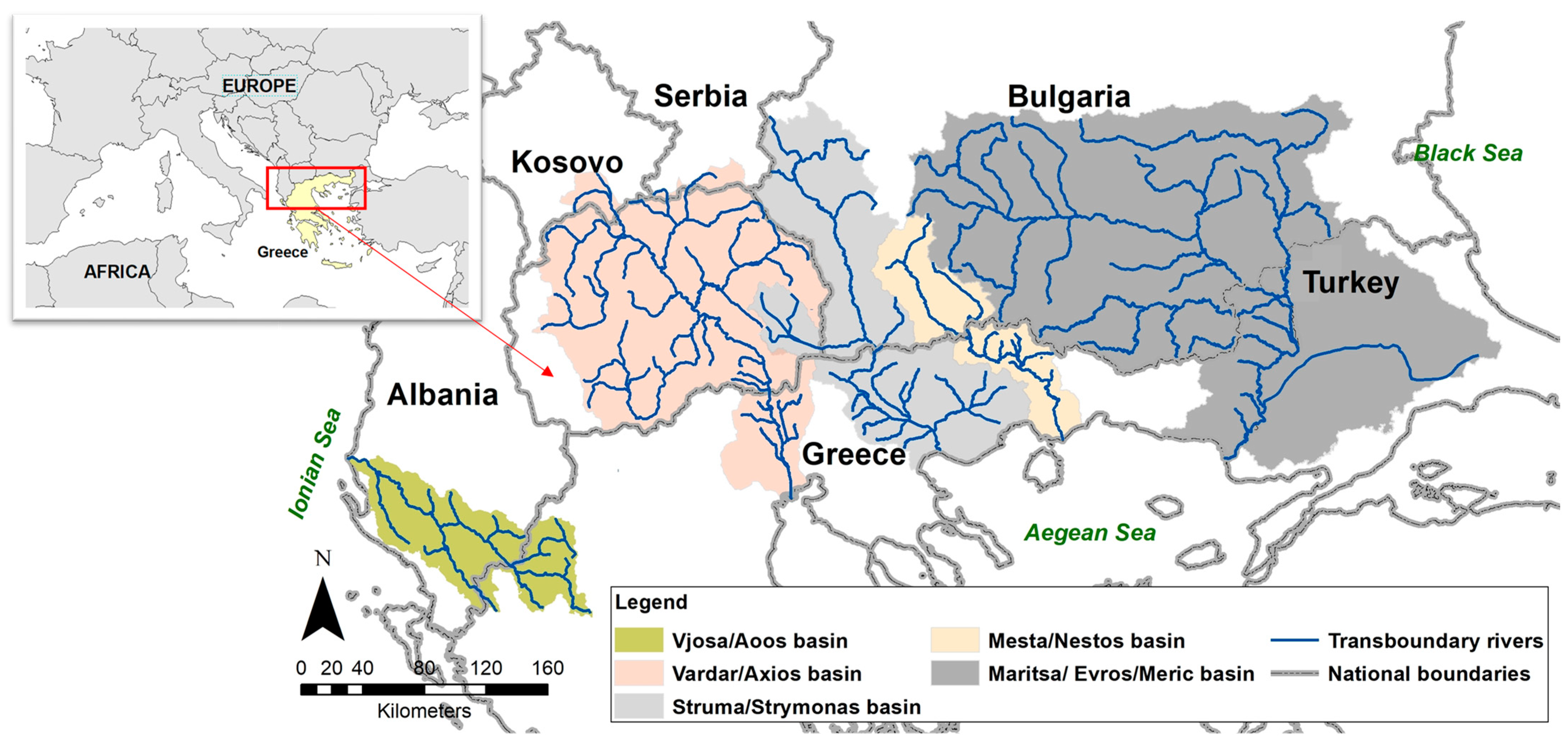
The case study area consists of the transboundary basins of Greece. Since Greece is located at the southern tip of the Balkan Peninsula (Figure 1), it serves as the natural conduit for the drainage into the North Aegean Sea from four rivers, each with its headwaters originating in upstream neighboring countries. At the same time, Greece is the source of an additional transboundary river, transcending national borders and draining into the North Ionian Sea. In a westward progression, Greece is the downstream country of the Maritsa/Evros/Meriç, Mesta/Nestos, Struma/Strymonas, and Vardar/Axios river basins, while it is the upstream country in the Vjosa/Aoos river basin case (Figure 1). Politically, more than 30 groundwater bodies are also identified that are shared with the same countries [28].

Figure 1.
Geographical illustration of the transboundary rivers shared between Greece and other riparian states.
The largest basin both in terms of areal coverage and population is the Maritsa/Evros/Meriç basin, with an extent of 53,475 km2 and more than 2 billion inhabitants (Table 1), followed by the Vardar/Axios basin, which covers 22,250 km2 and is populated by 1.77 million people. On the other hand, the Mesta/Nestos basin is the smallest basin, with an area of 5619 km2 and approximately 0.176 million people. In terms of river discharge and based on the literature data, the Maritsa/Evros/Meriç river has the highest outlet flow at 267.0 m3/s, while the Vardar/Axios river follows with 204.0 m3/s. Detailed river outlet data are provided in Section 3.1 for easier comparison with LSM-derived data.

Table 1.
Characteristics of the transboundary river basins of Greece.
From the five riparian countries of the case study basins (Table 1), only Greece and Bulgaria are EU Member States, meaning that only these two countries have a common water-related policy. Historically, as clearly stated in the 2nd Assessment of Transboundary Rivers, Lakes and Groundwaters [29], there were problems among the riparian countries regarding the quality (degraded water inflows) and quantity (excess water volumes) of these international waters. However, recent advancements, such as the creation of a Joint Expert Working Group between Bulgaria and Greece working on issues of the common development of RBMPs [30], the official solution of North Macedonia’s naming dispute with Greece [5], and the accession process of Albania and North Macedonia to the EU, which signifies, amongst other factors, the compliance of their national legislation with the WFD, have started casting light on the water-related disputes.
2.2. Large-Scale Hydrological Models and Data Sources
In this research, we used the simulation outputs of two well-established large-scale hydrological models (LSMs) at the European scale, namely the E-HYPE and the LISFLOOD models. E-HYPE [31] is the European version of the HYdrological Predictions for the Environment (HYPE) distributed hydrological model developed at the Swedish Meteorological and Hydrological Institute [32]. The model divides the 8.8 million km2 of Europe into 35,408 catchments, and all the data necessary for setting up the model, such as the hydrographic network of each watershed, land uses, and soil types, derived from validated open data sources [33]. Similarly, the daily mean precipitation and temperature required for the forcing of the model are from the open access WFDEI (WATCH Forcing Data–ERA-Interim) dataset, i.e., an enhanced version of the ERA-Interim data [34]. The model outputs consist of historic daily river discharges at the outlets of the designated catchments covering a time period of 30 years, i.e., January 1981 to December 2010. The calibration of E-HYPE is based on numerous discharge stations, while independent stations are used for its validation [33]. The literature review demonstrates that the E-HYPE model has been reviewed and validated at various spatiotemporal scales [9,35,36].
Regarding the LISFLOOD model, it was initially launched as the hydrological model of the European Flood Alert System (EFAS), i.e., an integrated system for medium-range flood forecasting at the European scale, developed by the European Commission Joint Research Centre (JRC) [37]. LISFLOOD is actually a hybrid model that combines both conceptual and physical rainfall-runoff components, coupled with a routing module in the river channel [38]. Thus, it is currently being routinely used for river basin hydrology, and assessment of river regulation effects, climate, and land use changes [39]. Operationalized on a squared 5 × 5 km grid, LISFLOOD employs spatially distributed input parameters and variables derived from European databases, such as the JRC MARS and the EU-FLOOD-GIS databases [40]. Static inputs, such as topography, soil type, land use, channel geometry, and river network, are also sourced from global databases, with soil properties, for instance, obtained from the European Soil Geographical Database. The model calibration is based on 693 stations, while the Standard Particle Swarm 2011 (SPSO-2011) algorithm was used to define the optimum parameters during the calibration phase [37]. The model has produced daily discharge data spanning from January 1992 to December 2022. Its effectiveness in simulating river basin dynamics has been demonstrated by numerous researchers (e.g., [41,42,43,44]).
The delineation of the transboundary basins into upstream and downstream waters is based on the political borders between riparian states. In the case of E-HYPE, the model’s catchments align with the border lines; therefore, water drained in these specific catchments represents upstream discharges. The LISFLOOD model, on the other hand, is a spatial distributed model with a 5 × 5 km grid. Thus, the grid cell representing the river’s course at national boundaries corresponds to the waters entering the downstream country. The runoff data sources used for the validation of the applicability of the large-scale hydrology models in the case study transboundary basins are derived from (i) the 1st revision of the RBMPs of the River Basin Districts of Epirus (EL05), Central Macedonia (EL10), Eastern Macedonia (EL11), and Thrace (EL12) (e.g., [45,46]), which contain the official hydrological data of Greece; (ii) the 2nd Second Assessment of Transboundary Rivers, Lakes and Groundwaters [29], which contains interannual averaged river discharge figures in both parts of a transboundary basin; and (iii) the Global Runoff Data Centre (GRDC) [47], which is an international hydrological data and information repository under the auspices of the World Meteorological Organization, with its data being used by numerous scholars [48,49]. All the aforementioned data are publicly available on the internet, with their sources given in the “Data availability statement” section. Lastly, the analysis of the LSMs data spans from January 1992 to December 2010, representing the common time period shared by LISFLOOD and E-HYPE.
2.3. Bias Correction and Output Validation
The bias correction of the LSMs’ outputs vs. the observation was conducted with the use of four methods, namely, scaling factor, linear regression, delta change, and quantile mapping. All the bias-correction calculations were employed with the use of the Python programming language. The scaling factor (SF) method aims to perfectly match the long-term monthly mean of simulated values with those of observed values [50]. Actually, the method calculates a scaling factor for multiplying the data that need to be corrected. The scaling factor is the ratio of the standard deviation of the observed data to the standard deviation of the simulated data and is expressed through the following equation:
where represents the bias-corrected discharges, Sf is the scaling factor, and represent the standard deviation of the observed and simulated data, respectively, and represents the simulated discharges.
In the linear regression (LR) method, the relationship between the observed and simulated data is formulated through a linear regression model [51]:
where represents the observed data, a is the intercept, and β is the slope. Then, the method calculates the optimal values of intercept and slope parameters that best fit the relationship between the independent and the dependent variable, and calculates the bias-corrected time series .
The delta change (DC) method, also known as the scaling factor or scaling coefficient method, uses a function for delta change multiplicative correction, and in our case the function is expressed as [52]:
where is the ratio between observed and simulated data (), where and represent the difference between consecutive observed and simulated values, respectively.
Quantile mapping (QM) is a statistical method used for adjusting the cumulative distribution function (CDF) of a model’s output to match that of observed data [53]. The main idea is to correct biases and discrepancies in the simulated data by aligning their quantiles with those of the observed data. In our case, after shorting the data, we calculate the quantiles for both datasets, dividing them into intervals of equal probability. Then, a mapping function (linear interpolation) is employed to map simulated quantiles to observed quantiles and the simulated data are adjusted accordingly. It can briefly be summarized through the following mathematical function [54]:
where the observed variable, is the modeled variable, is the CDF of , and is the inverse CDF corresponding to .
Finally, to assess the performance of the LSMs’ outputs in the case study basins, we performed goodness-of-fit quality checks, i.e., comparisons between the simulated outputs (before and after the bias correction) and the measured data (whenever and wherever it was feasible). To do so, the coefficient of determination (R2), the Percent Bias (PBIAS), Nash–Sutcliffe Efficiency (NSE) coefficient, Root-Mean-Square Error (RMSE), and the Kling–Gupta Efficiency (KGE) statistical measures were adopted. The specific statistical measures are routinely used in hydrology (e.g., [55,56]).
3. Results
3.1. Upstream Waters’ Contribution to Total Discharges
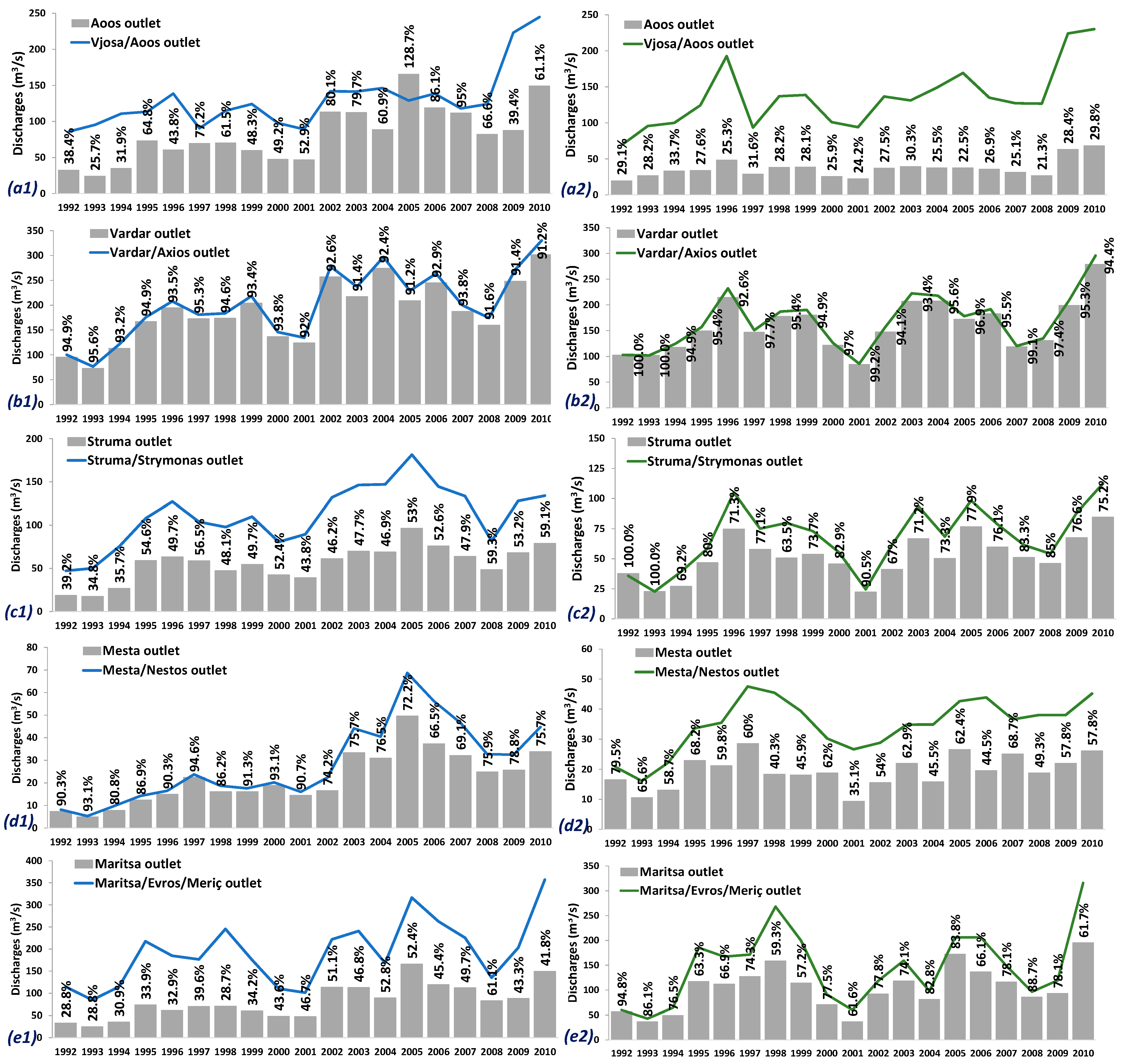
Initially, to identify the dependance of the downstream country to the upstream waters per basin, and as attributed by the large-scale models, we compared the upstream waters discharged at the political borders of the riparian states with the total river discharges at the outlets of the transboundary basins. In the Vjosa/Aoos river basin, the LISFOOD model shows that 63.04% of the waters come from the upstream basin (Figure 2(a1)), while the E-HYPE model shows a relatively smaller percentage of 27.21% of incoming waters (Figure 2(a2)).
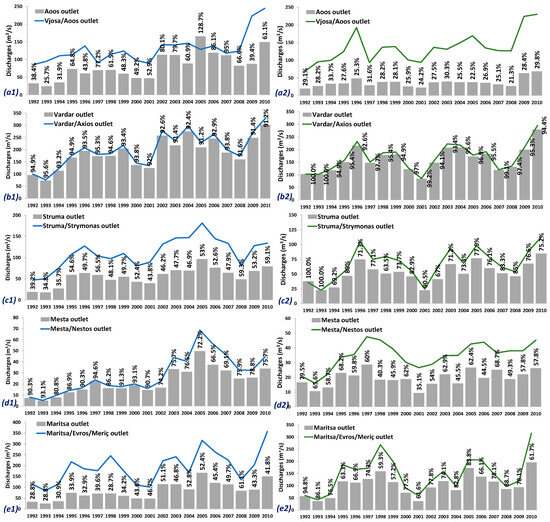
Figure 2.
Combined diagrams for demonstrating the contribution of the upstream parts of a basin (grey columns) to the total river discharges of the transboundary basins. The blue curves and the figures (a1–e1) correspond to the LISFLOOD simulations, and the green curves and figures (a2–e2) correspond to the E-HYPE model for the period 1992–2010.
For the Vardar/Axios river, LISFLOOD indicates a significant dependance of 92.84% on upstream waters (Figure 2(b1)). This dependency is of a similar magnitude to the 95.77% dependence on upstream waters depicted by the E-HYPE model (Figure 2(b2)). In the Struma/Strymonas basin, LISFLOOD shows that 49.97% of the water comes from upstream (Figure 2(c1)), while this percentage equals 76.52% in the case of the E-HYPE model (Figure 2(c2)). For the Mesta/Nestos basin, the simulated inflows to the downstream basin equal 77.95% and 55.86% for LIFLOOD (Figure 2(d1)) and E-HYPE (Figure 2(d2)), respectively. Finally, in the Maritsa/Evros/Meriç basin, the LISFLOOD and E-HYPE models do not converge, indicating that approximately 42.53% and 70.91% of the total river discharges originate from the upstream parts of the basin, respectively (Figure 2(e1,e2), respectively).
In terms of absolute figures for the period 1992–2010, as presented in Table 2, LISFLOOD significantly overestimates the runoff of the Vardar/Axios basin (201.44 m3/s vs. 132.71 m3/s respectively), while it underestimates the Vjosa/Aoos runoff (129.85 m3/s vs. 204.10 m3/s respectively). It exhibits a similar order of magnitude to the literature sources regarding the Struma/Strymonas basin (around 100.0 m3/s), while in all other cases it underestimates the interannual averaged discharges at the basins’ outlet. As far the E-HYPE model is concerned, Table 2 depicts that the model’s simulated outflows also significantly underestimate the Vjosa/Aoos runoff (135.48 m3/s vs. 204.10 m3/s, respectively), and slightly overestimate the Vardar/Axios runoff (167.68 m3/s vs. 132.71 m3/s, respectively). In all other basins, the model consistently undervalues the discharges, with the larger variation, i.e., approximately 50% less than the recorded values, occurring in the Maritsa/Evros/Meriç basin. It should be clearly mentioned that the runoff from the RBMPs and literature sources are cited figures that do not specify the period they concern. However, the author decided to present these figures since they mainly originate from the River Basin Management Plans and UNECE’s 2nd Assessment Report, demonstrating an order of magnitude of the transboundary river discharges. In the following sections, the observed discharges used in the analysis come from publicly available databases where information about the station’s location, observation timestep, and time series duration are available.
Table 2.
Averaged interannual discharges from the utilized LSMs (period 1992–2010) and literature sources, at both the basins’ borders and outlets.
3.2. Basins’ Climatology and Transboundary Rivers Discharges per LSM
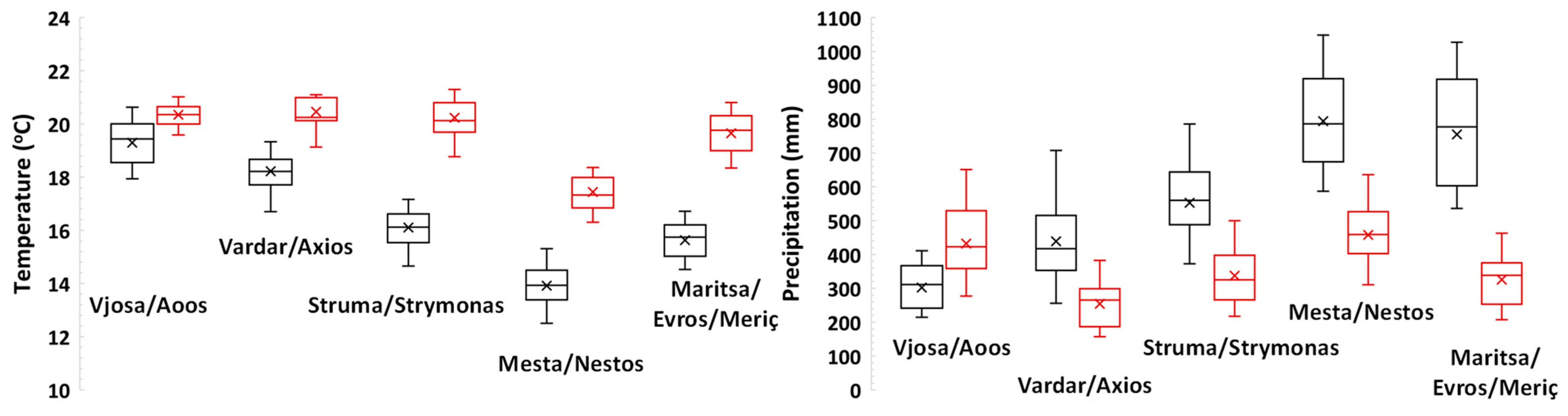
In terms of the regional climatology per basin and based on the ERA5 Land dataset [57], the areas of the basins in proximity to the Mediterranean Sea exhibit a more arid climate compared to the relatively sub-continental climate of the upper basins, as also shown by other scholars [58]. Specifically, as depicted in Figure 3, temperatures in all the downstream parts of the basins (red-colored boxplots) are higher than those in the upstream parts (black-colored boxplots). The larger differences are observed in the basins shared between Bulgaria and Greece, ranging between 3.52 and 4.12 °C, as the waters of these basins originate in the Rhodope mountains, which constitute the highest reliefs in the Balkans. The smaller temperature differences of approximately 1.1 °C are observed between the upper and lower part of the Vjosa/Aoos basin. Regarding precipitation, significant differences in rainfall are evident between the upper (black-colored boxplots) and lower parts (red-colored boxplots) of all the case study basins. The most pronounced differences are observed in the Mesta and Maritza basins, which receive interannual rainfall of approximately 795 mm and 755 mm, respectively, compared to the 460 mm and 330 mm of rainfall observed in the downstream Nestos and Evros basins.
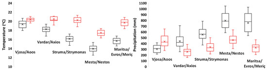
Figure 3.
Boxplot diagrams illustrating the interannual temperature (left-hand plots) and rainfall (right-hand plots) comparisons between the upper (red-colored plots) and lower (black-colored plots) parts of the five transboundary case study basins for the period 1992–2010.
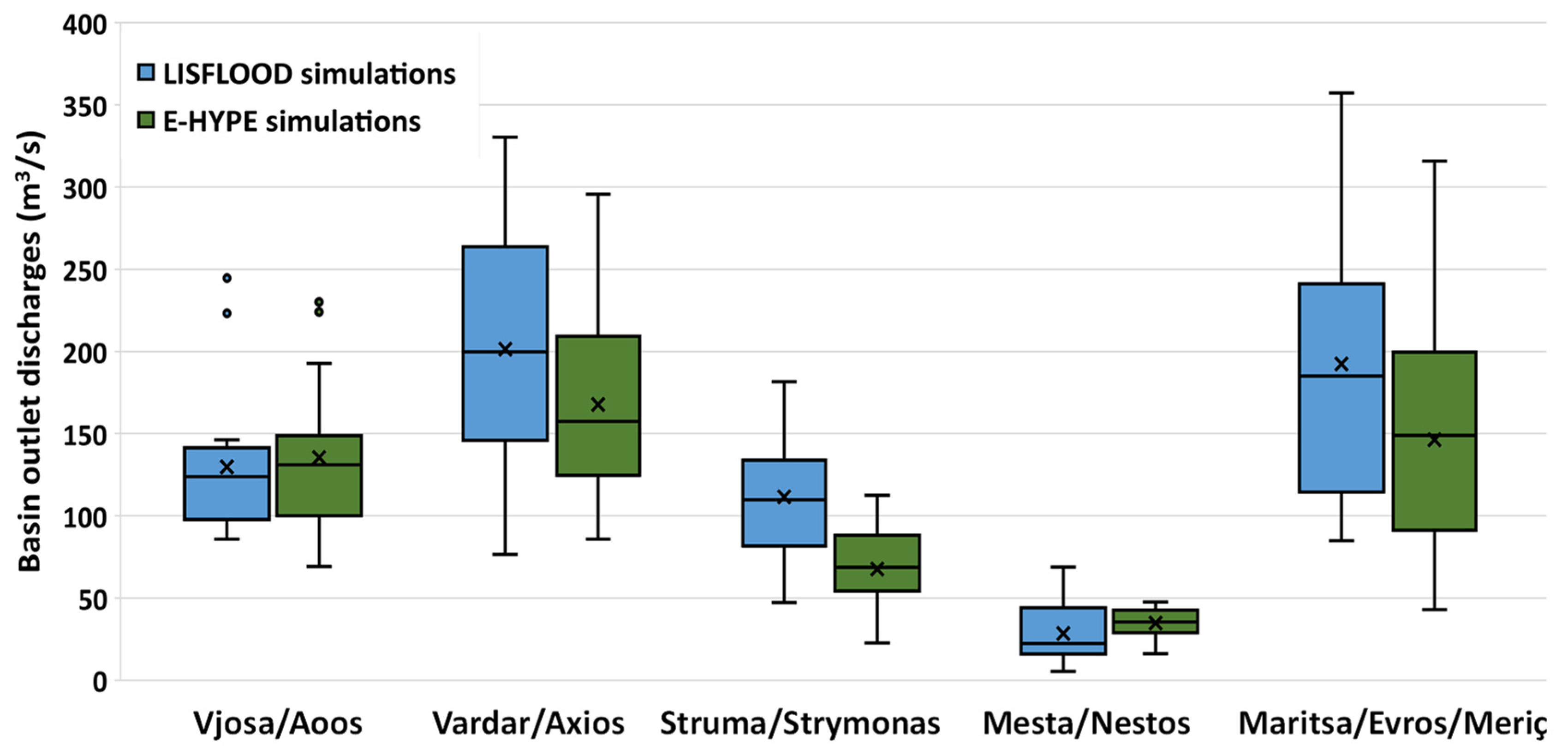
As for the LSMs’ simulated runoffs, disparities between the outputs of the two models are initially evident, particularly in the Struma/Strymonas and Mesta/Nestos basins. Figure 4 illustrates these differences, depicting the averaged interannual discharges in the form of boxplots, where the mean (the x sign within the boxes), median, lower and upper quartiles, and outliers are displayed. Specifically, the maximum runoff of the Struma/Strymonas River is 181.59 m3/s for the LISFLOOD model (depicted by blue boxplots in Figure 4) and 112.26 m3/s for the E-HYPE model (depicted by green boxplots in Figure 4), indicating an approximately 50% difference in favor of the former. Similar disparities are also observed in the case of monthly mean runoffs where LISFLOOD’s and E-HYPE’s discharges are 178.43 m3/s and 259.72 m3/s, respectively. In addition to the maximum values, LISFLOOD demonstrates an average interannual runoff of 111.46 m3/s, nearly twice the value of E-HYPE’s average of 67.05 m3/s. Notably, the lower whisker of LISFLOOD’s discharges is approximately equivalent to the E-HYPE’s the 3rd quartile (Q3), underscoring the magnitude of differences between the two models’ outputs.
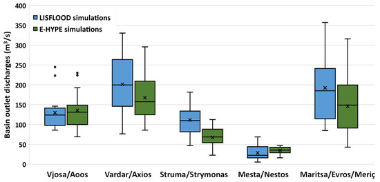
Figure 4.
Simulated averaged interannual discharges’ characteristics derived by the LISFOOD and E-HYPE models for the time period 1992–2010 at the outlets of the transboundary rivers in Greece.
The main difference in the performance of the LSMs within the Vardar/Axios river basin primarily lies in the occurrence of maximum values, with a difference of approximately 35.5 m3/s in favor of the LISFLOOD model. Despite the relatively small difference in median values of the two LSMs, which are 199.68 m3/s and 157.45 m3/s for LISFLOOD and E-HYPE, respectively, this difference is amplified in the case of the third quartile (Q3). In this regard, the upper limit of the Q3 values for LISFLOOD and E-HYPE are 263.89 m3/s and 209.31 m3/s, respectively. Nonetheless, both LSMs consistently project minimum average discharges of approximately 80.0 m3/s.
As for the Vjosa/Aoos basin, both LSMs present similar mean (approximately ±130.0 m3/s) and median values (approximately ±125.0 m3/s). Moreover, both models estimate that the maximum river discharges range between 230.0 m3/s and 244.0 m3/s, which are represented as outliers in the boxplot shown in Figure 4. In terms of minimum values, LISFLOOD simulations indicate that the interannual minimum runoff equals 85.9 m3/s, in comparison to 69.2 m3/s of the E-HYPE model.
Regarding the Mesta/Nestos basin, which has the smallest outflows of all five transboundary basins, LISFLOOD-simulated discharges range from 5.3 m3/s to 68.7 m3/s, while E-HYPE simulations range from 16.1 m3/s to 47.5 m3/s. The water volume ranges become even narrower when focusing on the values packed between the first (Q1) and third quartiles (Q3), as clearly depicted in Figure 4.
Lastly, given the vast extent of the Maritsa/Evros/Meriç basin, both LSMs exhibit similar performance indices, with the LISFLOOD model showing slightly overestimated discharges compared to E-HYPE. Specifically, LISFLOOD’s maximum and minimum interannual discharges are 357.3 m3/s and 84.8 m3/s, respectively (upper and lower whiskers), while E-HYPE’s maximum and minimum discharges are 315.8 m3/s and 42.9 m3/s, respectively, as indicated by the upper and lower whiskers of the corresponding boxplots in Figure 4. On the other hand, the performed analysis at monthly time scale (not shown here) reveals that LISFLOOD’s maximum discharge of 918.8 m3/s is almost half of E-HYPE’s 1674.9 m3/s.
3.3. Bias-Corrected LSM Outflows and Comparison to Measurements
The implemented methodology for bias correction of the LSMs outputs was fully applied only to the Vardar/Axios and Mesta/Nestos basins, where measured discharges were available for the same time period with the LSMs. For the Struma/Strymonas and the Maritsa/Evros/Meriç basins, the available data are compared only with E-HYPE’s outflows because the observation datasets had a relatively short (60 months) mutual temporal coverage. As for the Vjosa/Aoos basin, no published runoff time series were identified; thus, we conducted an intercorrelation analysis between the two LSMs to investigate their performance.
3.3.1. Vardar/Axios Basin
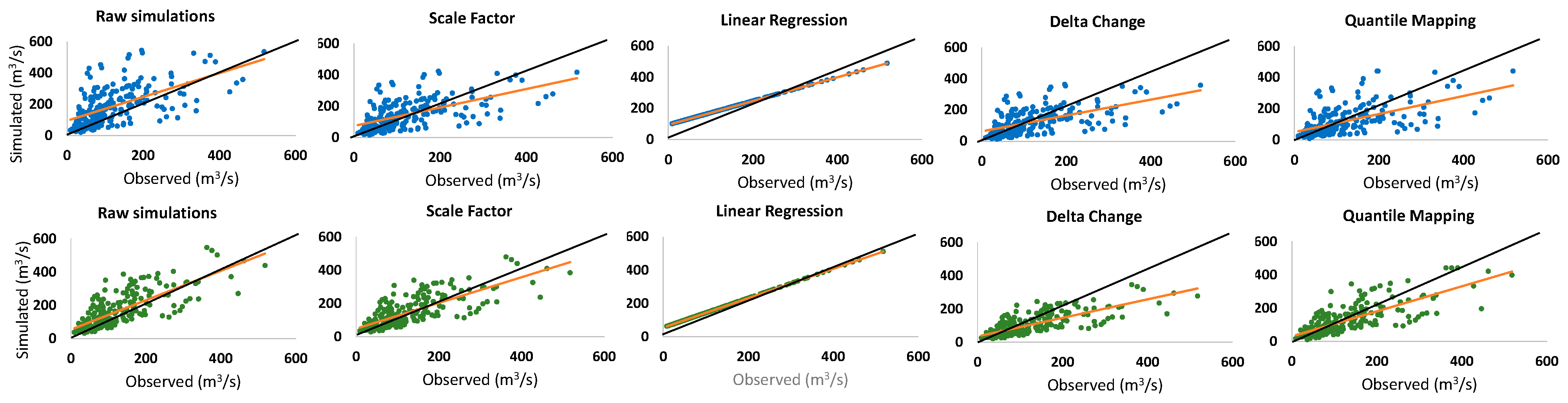
Starting with the Vardar/Axios basin, the common dataset spans from January 1992 to December 2010 (number of samples: n = 228), with observed discharges spatially measured just a few kilometers upstream (location: Gevgelija City, latitude: 41.147598, longitude: 22.523647) of the borders, and practically corresponding to the discharges of the North Macedonian part of the basin. Regarding the LISFLOOD model, the comparison of the observed and simulated runoff, depicted as the “Raw simulations” blue plotted points in Figure 5, illustrates a relatively good correlation between the two time series. The numerical representation of this correlation, as well as those generated after applying bias-correction techniques, is provided in Table 3, where the statistical measures indicate satisfactory initial values, for instance R2 = 0.349. The scale factor (SF) bias-correction technique as depicted by the relevant plot and the associated statistics significantly improves the correlation of the two time series (e.g., NSE = 0.111 instead of the initial negative value, and KGE=-0.657). The linear regression plot in Figure 5 corresponds to the linear regression (LR) bias-correction method and, while the R2 value is as expected at 1.0, other indices remain above 0.4, for example, NSE = 0.423 and KGE = 0.403. Similarly, both the delta change (DC) and quantile mapping (QM) techniques improve the relationship between the two datasets, with all statistical measures being accepted (in both cases NSE ≥ 0.34 and KGE ≥ 0.57). It should be noted that single basin model streamflow simulations are considered satisfactory when NSE > 0.50 and PBIAS = ±25%, as clearly mentioned by Moriasi et al. [59]. However, for multi-basin calibration and validation, i.e., the case of LSMs, these thresholds are slightly lower, as highlighted in the Section 4, since the models’ performance is based on the overall output of these statistical indicators.
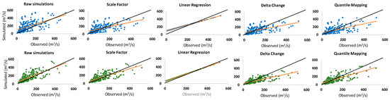
Figure 5.
Comparison of observed runoff with simulations of LISFLOOD (blue plotted points) and E-HYPE (green plotted points) for the Vardar/Axios basin. Raw simulation plots (first column of plots) show the data before their bias correction, while subsequent columns display bias-corrected data per method. The orange curve represents the linear feet, and the black curve denotes the 1:1 slope.
Table 3.
Performance of bias-correction methods in the case of the Vardar/Axios river’s LISFLOOD-simulated runoff expressed through statistical measures.
It should be noted that the coefficient of determination (R2) of the SF and DC methods equals the one obtained when comparing measured and raw discharges. This occurs because the bias-corrected time series produced by these two methods maintain a linear relationship with the initial LSM simulations, as expressed by Equations (1) and (4), respectively. Therefore, in all the relevant tables, the R2 value among these specific methods will be equal to that of the raw data.
For the E-HYPE model, the statistical comparison between observed and simulated data reveals a significant correlation between the two datasets, with R2 and KGE being larger than 0.5, as presented in Table 4. Despite the low initial NSE value of 0.268, all statistical indexes improve after the bias-correction process. In the SF method, NSE increases to 0.497, PBIAS is halved, KGE reaches 0.719, and RMSE falls to 41.412 m3/s. Similarly, high correlation indexes are observed in the LR and DC methods, with NSE values of 0.797 and 0.548 respectively, while KGE exceeds 0.6 in both methods. Satisfactory results are also achieved with the QM method, where R2, NSE, and KGE are all above 0.55 in every case, and PBIAS is very close to zero.
Table 4.
Performance of bias-correction methods in the case of the Vardar/Axios river’s E-HYPE-simulated runoff expressed through statistical measures.
3.3.2. Mesta/Nestos Basin
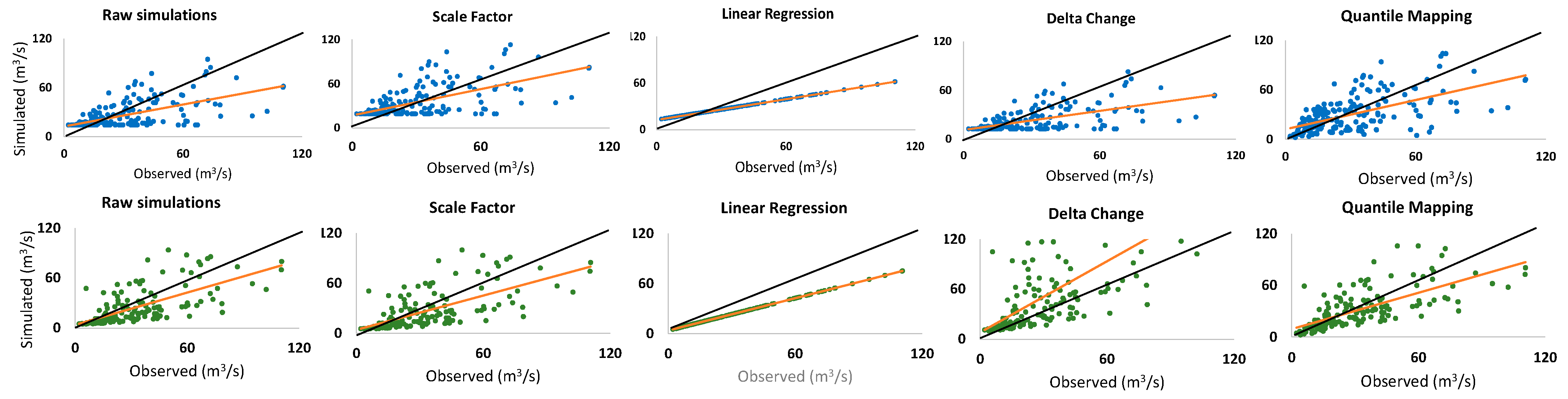
The comparison of the monthly averaged LISFLOOD discharges with observed data received just a few kilometers downstream the Greek–Bulgarian border (location: Thissavros dam latitude: 41.382363, longitude: 24.080333) for the period November 1997–December 2010 (n = 158) demonstrates an initially good correlation between the two time series, as shown in the upper left scatter plot of Figure 6. As observed in the specific figure, LISFLOOD’s minimum runoff is approximately 14.5 m3/s and is repeated frequently (numerous points at the same level of the y-axis), meaning that the model has a low-flow threshold that cannot be surpassed. On the other hand, one-third of the recorded flows vary from 2.19 m3/s to 14.5 m3/s, indicating the inability of the model to assess the basin’s low discharges. This minimum threshold affects the performance of the implemented bias-correction techniques, as is clearly apparent in the remainder of the blue plotted points. Only the QM and LR methods seems to overcome this shortcoming, where the bias-corrected time series are much better correlated with the records (e.g., KGE > 0.4 in both cases). The statistical measures of the specific plots, as presented in Table 5, confirm the average correlation, as R2 equals 0.35 and both NSE and KGE range between 0.21 and 0.6 in all cases.
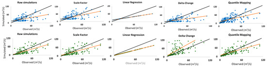
Figure 6.
Comparison of observed runoff with the simulations of LISFLOOD (blue plotted points) and E-HYPE’s (green plotted points) for the Mesta/Nestos basin. The first column of plots shows the data before their bias correction, while subsequent columns display bias-corrected data. The orange curve represents the linear feet, and the black curve denotes the 1:1 slope.
Table 5.
Performance of bias-correction methods in the case of the Mesta/Nestos river’s LISFLOOD-simulated runoff expressed through statistical measures.
On the other hand, E-HYPE’s raw outputs demonstrate a satisfactory correlation with the observed discharges, as depicted by the first plot with green points of Figure 6. This correlation is further increased when some of the bias-correction methods are implemented. For the QM method, the initial R2 of 0.473 increases to 0.501, accompanied by an increase in KGE from 0.604 to 0.708, as shown in Table 6. In the LR method, the produced time series have an increased NSE indicator reaching 0.772, the KGE is 0.574, and the RMSE falls to 10.938 m3/s. The SF method yields outputs with statistical measures close to those of the raw data, while the DC method fails to produce acceptable statistical indicators.
Table 6.
Performance of bias-correction methods in the case of the Vardar/Axios river’s E-HYPE-simulated runoff expressed through statistical measures.
3.3.3. Struma/Strymonas Basin
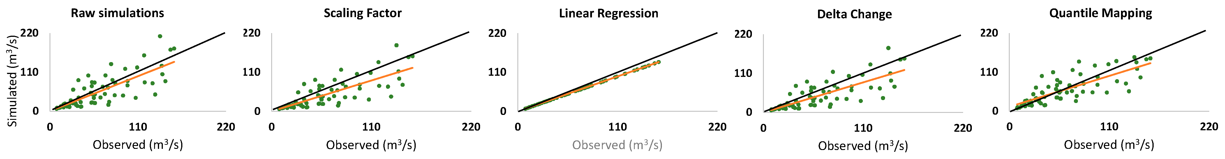
The monitored discharges for the Struma/Strymonas basin are available for the period January 1981–December 1986 (n = 72) and they originate from a Bulgarian station (location: Marino Pole, latitude: 41.41666, longitude: 23.35) just upstream of the political borders of the riparian states. Hence, the available datasets’ time coverage only allows statistical analysis of E-HYPE’s simulated discharges, as LISHFLOOD data are only available from January 1992. As illustrated in Figure 7, the comparison between the model’s raw output with the observed flows demonstrates a strong performance, with R2 and KGE indexes exceeding 0.61. Additionally, NSE equals 0.472 and RMSE is 28.951 m3/s (Table 7). The SF and DC bias-correction methods result in a slight improvement in the correlation indexes, with NSE values of 0.475 and 0.476 respectively. However, the comparison indexes remain very similar to the initial ones. The QM method outperforms the previous two methods, with all indexes falling within the range of increased correlated datasets, i.e., R2 = 0.629, NSE = 0.589, KGE=-0.793, and PBIAS is almost equal to zero. The LR method yields the best bias-correction results, with an NSE of 0.965, a KGE of 0.852, and an RMSE of 7.448 m3/s (Table 7). These values demonstrate the LR method’s capability of producing bias-corrected discharges that are highly correlated with the observation records. However, it is worth noting that the relatively short temporal coverage of the measurements and their age necessitates the further evaluation of the produced linear regression’s slope and intercept factors in recent years.
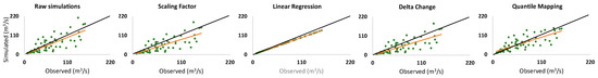
Figure 7.
Comparison of observed runoff with E-HYPE’s raw and bias-corrected simulations for the Struma/Strymonas basin. The orange curve represents the linear feet, and the black curve denotes the 1:1 slope.
Table 7.
Performance of bias-correction methods in the case of the Struma/Strymonas river’s E-HYPE-simulated runoff expressed through statistical measures.
3.3.4. Maritsa/Evros/Meriç Basin
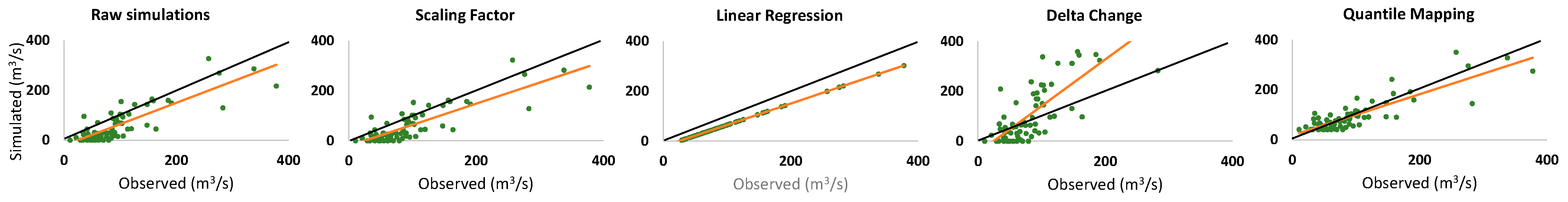
Similar to the Struma/Strymonas basin, the available observations of the Maritsa/Evros/Meriç river basin date to the period January 1981–December 1986, comprising n = 72 monthly samples. Therefore, the conducted analysis focuses on the E-HYPE model. However, it is important to note that the monitoring station is situated in the Maritsa part of the basin (location: Svilengrad village, latitude: 41.766666, longitude: 26.2000), just above the Greek–Bulgarian border. As a result, the data obtained from this station do not include the runoff of the Tundja, Arda, and Ergene river basins, which are the larger tributaries of this transboundary river.
The correlation between observations and E-HYPE’s simulations, as depicted in Figure 8, is impressively good. The trend curve closely follows and parallels the 1:1 slope of the axes, as indicated by the orange and black curves in Figure 8. Furthermore, the bias-correction techniques maintain the same visual performance, apart from the case of the delta change method.
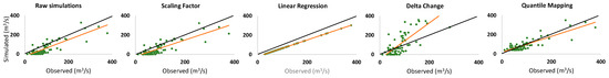
Figure 8.
Comparison of observed runoff with E-HYPE’s raw and bias-corrected simulations for the Maritsa/Evros/Meriç basin. The orange curve represents the linear feet, and the black curve denotes the 1:1 slope.
In terms of absolute figures, the outputs between the observed and unbiased discharges, as indicated by R2 = 0.714 (see Table 8), and the other statistical measures, such as a fair NSE (= 0.444), a quite high KGE (= 0.602), and a RMSE of 54.499 m3/s (considering that the maximum flow of the river is 377.89 m3/s), denote a relatively good correlation in the time series. The comparison of outputs between the observed and the produced LR and QM modified discharges revealed that these two methods generate the less biased time series. LR demonstrates a strong correlation, with all indices exceeding 0.6 (NSE = 0.737 and KGE = 0.616), as shown in Table 8. On the other hand, the QM method produces time series that are even more correlated, with all statistical measures surpassing 0.74 (R2 = 0.749, NSE = 0.761, and KGE = 0.856). Moreover, both LR and QM yield RMSE values (RMSE = 36.097 m3/s and RMSE = 35.816 m3/s) that are considered good since they are less than half of the measured standard deviation [60]. Nevertheless, due to the limited duration and aging of the measurements, it is crucial to reassess the linear regression’s slope and intercept factors in recent years for the specific river basin.
Table 8.
Performance of bias-correction methods in the case of the Struma/Strymonas river’s E-HYPE-simulated runoff expressed through statistical measures.
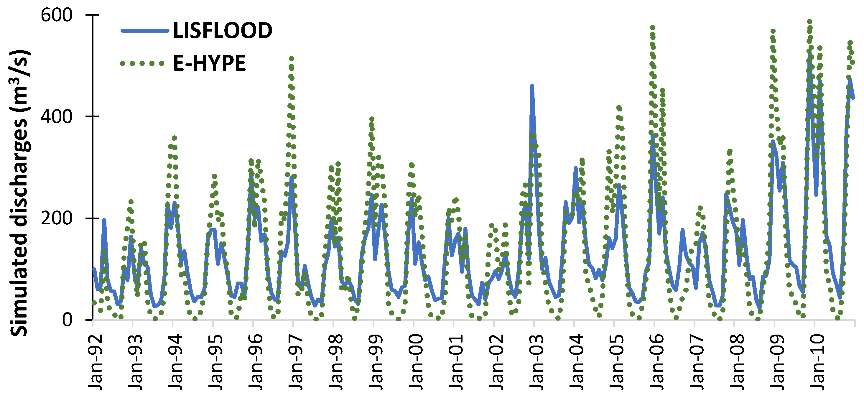
3.3.5. Vjosa/Aoos Basin
Due to the lack of monitored discharges in the Vjosa/Aoos basin, a qualitative comparison of the two LSMs datasets was conducted during the common period of data, spanning from January 1992 to December 2010 (n = 228), as illustrated in Figure 9. While both models capture the seasonal discharge variability similarly, a notable difference is detected in LISFLOOD outputs, which exhibit a low-flow threshold, i.e., the minimum value of the river runoff does not drop below approximately 25.0 m3/s. Overall, it can be observed that the specific model outputs feature lower peaks and less pronounced fluctuations compared to those of E-HYPE. Furthermore, it is important to note that the figures cited in the literature regarding the rivers’ runoff, as outlined in Table 2, can only be examined quantitatively. This is because the time period for which these average flows were generated is unspecified; they may thus correspond to wet or dry periods, potentially resulting in overestimated or underestimated river discharges, respectively. Regardless of the case, the literature indicates that the average Vjosa/Aoos river’s outlet flow into the Ionian Sea is 204.10 m3/s, approximately 34% larger than the 129.85 m3/s and 135.48 m3/s estimated by the LISFLOOD and E-HYPE models, respectively.
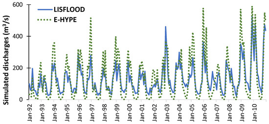
Figure 9.
LSMs’ simulated discharges at the outlet of the Vjosa/Aoos river for the period January 1992–December 2010.
Overall, in Table 9, we present the statistical numerical outputs of the observed time series, including minimum and maximum values (excluding outliers), first and third quantiles, and median and mean discharges. Additionally, the table includes the initial (raw) simulations of LISFLOOD and E-HYPE models, as well as the bias-corrected simulated time series generated using the LR and QM methods, which have demonstrated superior applicability in the case study basins. In all basins, LR and QM methods contribute to convergence of the median and mean simulated values to the observational data. In the Vardar/Axios basin, for instance, the median and mean LISFLOOD-simulated values of 199.68 m3/s and 201.44 m3/s, respectively, are adjusted to 117.64 m3/s and 121.01 m3/s, respectively, which closely approximate the observed values, with a difference of ±1.5 m3/s. It should be noted that the time series presented in Table 9 do not correspond to the same period. As mentioned earlier, the statistics for the Struma/Strymonas and Maritsa/Evros/Meriç basins derive from a six-year period of data, whereas the statistics for the other two basins derive from data spanning a period more than double in length. Finally, the Vjosa/Aoos basin is not included in the table due to the lack of observations, which impeded the bias correction of the LSM’s simulated runoff.
Table 9.
Statistical measures of observed discharges (Obs.), LISFLOOD’s and E-HYPE’s raw simulations (Raw), and linear regression (LR) and quantile mapping (QM) bias-corrected time series for the transboundary basins of Greece based on the available time series of data. All data are expressed in m3/s.
4. Discussion
Within the present study, we assess the applicability of two large-scale hydrology models (LSMs), namely the LISFLOOD and E-HYPE models, in accurately representing water volumes, focusing on the five transboundary river basins of Greece. The literature indicates that only a very limited number of scholars have utilized and validated the performance of these models in Greece and in its international waters. For instance, Skoulikaris and Piliouras [9], and Skoulikaris [36], evaluated E-HYPE’s performance solely for the Vardar/Axios river basin, while Mentzafou et al. [61] used the specific model’s simulated discharges as those that occur in seven national rivers, but without any validation. Notably, although LISFLOOD outputs form part of the EU Climate Data Store produced by the European Flood Awareness System (EFWS) as part of the Copernicus Programme [62], the model has yet to be utilized and evaluated in Greece. At the same time, to the best of the author’s knowledge, none of the specific LSMs have been utilized by the riparian states sharing their waters with Greece. Hence, we consider our approach novel in (i) using two LSMs in the transboundary river basins of Greece, which cover a large area of the Balkan Peninsula, (ii) validating the performance of these LSMs for selective case studies, and thus proposing solutions for situations of data scarcity or in ungauged basins, (iii) demonstrating, for the first time with the use of long-term discharge datasets, the dependance of the downstream parts of the basins to the upstream waters, and (iv) advocating for the use of LSMs as tools for integrated management of international waters.
The data analysis demonstrated, as anticipated, varying performance among the selected LSMs (see Figure 4). However, in most case study basins, the simulated interannual mean and median flows align between the two models. Notably, there were cases, such as in the Struma/Strymonas river basin, where significant disparities, such as more than 50% difference in averaged discharges, were observed between the outputs. Additionally, it was found that, in certain basins, the LISFLOOD model employs a low-flow threshold, resulting in inadequate attribution of minimum flows. This finding aligns with the research conducted by Gudmundsson et al. [12], where the assessment of nine LSMs, forced by the same meteorological variables, against observed runoff from 426 small catchments in Europe, demonstrates that while LSMs generally capture the interannual variability of mean flow well, differences in model performance become more pronounced for low-flow percentiles. Additionally, Donnelly et al. [31] highlight that models’ outputs are improved with increasing catchment size due to the lesser impact of water regulation strategies on hydrosystem behavior compared to the frequent runoff peaks observed in smaller catchments.
Focusing on the two LSMs, although they are well-established and validated models, as clearly indicated in the Section 2, e.g., [9,35,41,42], none of the Greek national or international basin gauges, along with their relative gauges, have been utilized for validation during their development phase. Specifically, that of LISFLOOD uses only a station (out of the 693 utilized stations) in the upper part of the Struma basin for its validation [62], while E-HYPE validation does not include sub-Danubian basins [31]. In this regard, the research validates the two LSMs in the river basins of Southeastern Europe, demonstrating their potential to successfully simulate river discharges. The data analysis reveals that, in the Vardar/Axios basin, R2, NSE, and KGE are 0.349, −0.657, and 0.259 for LISFLOOD, and 0.595, 0.268, and 0.574 for E-HYPE (see Table 3 and Table 4). For the Mesta/Nestos basin, the goodness-of-fit measures indicate that R2, NSE, and KGE are 0.353, 0.301, and 0.507 for LISFLOOD, and 0.473, 0.308, and 0.604 for E-HYPE (see Table 5 and Table 6). The outputs of the E-HYPE model in both of the aforementioned case study basins coincide with those produced by the model during its development phase, as reported by Donnelly et al. [31]. It is indicated that, for all E-HYPE’s validation stations across Europe, two-thirds had NSE greater than zero, and one-third of the stations had values greater than 0.4, which aligns with our research findings. Additionally, Donnelly et al. [31] demonstrate that 85% of all validation stations across Europe had KGE greater than zero, with 52% having values greater than 0.5, a pattern consistent with the outputs of our current research. Regarding the LISFLOOD model, the model’s validation output demonstrates that 16% (97 out of 594 validation stations) had a negative NSE, while 78% (461 out of 594 stations) had NSE values greater than 0.2 [62], which is consistent with the findings of the current research. Finally, in the case of the Struma/Strymonas and Maritsa/Evros/Meriç basins, the absence of current observational data necessitated an examination solely of E-HYPE’s capability to represent river runoff. In both cases, the outputs (R2 = 0.619, NSE = 0.472, and KGE = 0.726 for the Struma/Strymonas basin, and R2 = 0.714, NSE = 0.444, and KGE = 0.602 for the Maritsa/Evros/Meriç basin) reveal E-HYPE’s ability to accurately simulate the river discharges. However, it is essential to re-evaluate the specific model using more recent data and longer time series, since small data samples increase the likelihood of observational errors, potentially resulting in biased outcomes during model evaluation [12].
In the bias-correction process, the methods utilized are commonly employed in surface hydrology and mathematical models’ evaluation (e.g., [50]). Bias-correction methods resulted in an overall increase in the statistical indexes, indicating the correlation between observed and bias-corrected data. The relatively straightforward linear regression (LR) method, for instance, performed very well in the case of the Vardar/Axios and Mesta/Nestos basins. Specifically, the initial NSE values of −0.657 and 0.301 for LISFLOOD (see Table 3 and Table 5) became 0.423 and 0.797, respectively, while in the case of the E-HYPE model, NSE increased from 0.268 and 0.308 for the Vardar/Axios and Mesta/Nestos basins to 0.664 and 0.772, respectively (see Table 4 and Table 6). The same method also performed very well in the case of the Struma/Strymonas and Maritsa/Evros/Meriç basins, where NSE and KGE values for both LSMs were greater than 0.73 and 0.61, respectively (see Table 7 and Table 8). The quantile mapping (QM) method also had a positive impact on increasing the statistical measures, and in some cases, outperformed other methods. In the case of the LISFLOOD model, for example, KGE is constantly greater than 0.58, and in the case of the E-HYPE model, KGE is greater than 0.7, which is the best indicator among the bias-correction methods. Moreover, QM resulted in PBIAS values very close to zero (<±1.0 for all cases) indicating the excellence performance of the method. Finally, the scaling factor (SF) and delta change (DC) methods provided less satisfactory outputs, concluding that LR and QM bias-correction techniques are efficient in decreasing the LSMs’ runoff biases in the case study basins.
An important output of the research is the quantification of the dependence of the downstream parts of the case study transboundary basins on the available upstream water resources. This analysis is also considered an innovative aspect of the study, as the literature review revealed a lack of gauge stations, an issue which aligns with the research of Skoulikaris and Pilirouas [9] at the national borders of transboundary basins, as well as a lack of documented figures (see Table 2) about the upstream inflows. Regarding the contribution of the upper parts of the basins, in the case of the Vjosa/Aoos river basin, LISFLOOD and E-HYPE attribute 63.04% and 27.2% of the basins’ waters to upstream sources, respectively. Considering only 33% of the basin’s area belongs to Greece, it can be said that LISFLOOD partially overestimates the water inflow into Albania. In the Vardar/Axios basin, both LSMs demonstrate that the inflows from North Macedonia correspond to more than 92% of the total inflows, establishing the significant dependence of the downstream water uses on upstream waters. As for the Struma/Strymonas and Mesta/Nestos basins, which are almost equally shared between Bulgaria and Greece, both LSMs coincide that approximately 50% to 75% of the waters originate from upstream sources. This result, particularly in the case of the Mesta/Nestos basin, is validated in the literature [30]. As far the Maritsa/Evros/Meriç basin is concerned, the LISFLOOD and E-HYPE models show that 42.53% and 70.9% of the basin waters, respectively, are coming from upstream sources. These figures are relatively small, particularly in the case of LISFLOOD, considering that Greece accounts for only 6.9% of the basin’s extent and is primarily comprised of plain areas. However, it should be noted that not all major tributaries of the river are connected in the upstream waters, and thus are not considered by the two models as upstream waters.
To sum up, the research promotes a methodology for producing realistic outputs regarding the water discharges of transboundary basins, which can further be used to trigger indexes demonstrating cooperative and conflictive interactions, such as those of the International Water Event Database (IWED) [63]. Moreover, the outputs can lay the foundation for cooperative water management and the development of a framework for addressing scarcity and dependency, as proposed by Munia et al. [64]. De Stefano et al. [65] provide a thorough analysis on the transboundary basins that are more likely to experience hydro-political tensions over the coming years due to construction of large hydraulic projects, such as dams within the river course. Hence, the analysis of large-scale construction impacts on transboundary water resources is considered the advancement of the current research. Moreover, De Stefano et al. [66] investigated the institutional resilience to water variability in transboundary basins due to climate change; thus, the investigation of transboundary water bodies’ vulnerability to climate change is also a thematic proposed to be further investigated. In terms of the research limitations, LSMs provide daily or mean simulated discharges rather than extremes [12]; thus, the proposed methodology cannot be followed in the case of extremal analysis.
5. Conclusions
Accurate data and effective data exchange are fundamental for ensuring equitable and sustainable management of transboundary waters. This significance is underscored by Article 6 of the Convention on the Protection and Use of Transboundary Watercourses and International Lakes [6], as well as Article 8 of the Draft Articles on the Law of Transboundary Aquifers [67]. Furthermore, the EU, through its Water Framework Directive, recognizes information sharing as a cornerstone of integrated water resources management at national and transboundary scales [68].
This research, in the absence of monitoring data, investigated the way LISFLOOD and E-HYPE large-scale hydrological models (LSMs) can represent the river discharges of the transboundary river basin of Greece. The E-HYPE model slightly outperformed the LISFLOOD model in most of the case study basins; however, more recent data are required to establish a more secure consideration. Overall, the outputs demonstrate that both models provide reliable outputs that are further ameliorated after correcting for bias. Among the methods used for creating unbiased time series, linear regression and quantile mapping produced outputs of high accuracy. The research is considered a methodological roadmap that can be implemented in basins where limited data are available, as well as in transboundary basins where the often-political environmental policies and frameworks between the riparian states do not facilitate the integrated modeling of the water resources.
This research, conducted in the absence of ample monitoring data, investigates how LISFLOOD and E-HYPE large-scale hydrological models (LSMs) represent the river discharges of the transboundary river basin of Greece. The E-HYPE model slightly outperforms the LISFLOOD model in most of the case study basins; however, more recent data are required to establish a more secure conclusion. Overall, the outputs demonstrate that both models provide reliable results, which are further improved after bias correction. Among the methods used for creating unbiased time series, linear regression and quantile mapping produced highly accurate outputs. The research serves as a methodological roadmap that can be implemented in basins with limited data availability, as well as in transboundary basins where political and environmental policies and frameworks between riparian states often do not facilitate the integrated modeling of water resources.
Funding
This research received no external funding.
Data Availability Statement
All the data used in the research are freely available on the internet. RBMPs of Greece: https://wfdver.ypeka.gr/en/management-plans-en/approved-management-plans-en/ (accessed on 14 December 2023). Global Runoff Data Centre: https://www.bafg.de/GRDC/EN/01_GRDC/grdc_node.html (accessed on 10 December 2023). E-HYPE: https://hypeweb.smhi.se/explore-water/historical-data/ (accessed on 10 December 2023). LISFLOOD: https://cds.climate.copernicus.eu/cdsapp#!/dataset/efas-historical?tab=overview (accessed on 25 November 2023). ERA5-Land reanalysis dataset: https://cds.climate.copernicus.eu/cdsapp#!/dataset/reanalysis-era5-land?tab=overview (accessed on 28 January 2024).
Conflicts of Interest
The author declares no conflicts of interest.
References
- Giordano, M.; Drieschova, A.; Duncan, J.A.; Sayama, Y.; De Stefano, L.; Wolf, A.T. A review of the evolution and state of transboundary freshwater treaties. Int. Environ. Agreem. Politics Law Econ. 2014, 14, 245–264. [Google Scholar] [CrossRef]
- Turhan, Y. The hydro-political dilemma in Africa water geopolitics: The case of the Nile river basin. Afr. Secur. Rev. 2020, 30, 66–85. [Google Scholar] [CrossRef]
- Bernauer, T.; Böhmelt, T. International conflict and cooperation over freshwater resources. Nat. Sustain. 2020, 3, 350–356. [Google Scholar] [CrossRef]
- de Bruin, S.P.; Schmeier, S.; van Beek, R.; Gulpen, M. Projecting conflict risk in transboundary river basins by 2050 following different ambition scenarios. Int. J. Water Resour. Dev. 2024, 40, 7–32. [Google Scholar] [CrossRef]
- Skoulikaris, C.; Zafirakou, A. River Basin Management Plans as a tool for sustainable transboundary river basins’ management. Environ. Sci. Pollut. Res. 2019, 26, 14835–14848. [Google Scholar] [CrossRef]
- UNECE (United Nations Economic Commission for Europe). United Nation Convention on the Protection and Use of Transboundary Watercourses and International Lakes. 1992. Available online: https://unece.org/DAM/env/water/publications/WAT_Text/ECE_MP.WAT_41.pdf (accessed on 10 January 2024).
- UNEP-DHI; UNE. Transboundary River Basins: Status and Trends; United Nations Environment Programme (UNEP): Nairobi, Kenya, 2016. [Google Scholar]
- Skoulikaris, C.; Krestenitis, Y. Cloud Data Scraping for the Assessment of Outflows from Dammed Rivers in the EU. A Case Study in South Eastern Europe. Sustainability 2020, 12, 7926. [Google Scholar] [CrossRef]
- Skoulikaris, C.; Piliouras, M. Hydrological simulation of ungauged basins via forcing by large-scale hydrology models. Hydrol. Process. 2023, 37, e15044. [Google Scholar] [CrossRef]
- Junqueira, A.M.; Mao, F.; Mendes, T.S.G.; Simões, S.J.C.; Balestieri, J.A.P.; Hannah, D.M. Estimation of River Flow Using CubeSats Remote Sensing. Sci. Total Environ. 2021, 788, 147762. [Google Scholar] [CrossRef]
- Salat, J.; Pascual, J.; Flexas, M.; Chin, T.M.; Vazquez-Cuervo, J. Forty-five years of oceanographic and meteorological observations at a coastal station in the NW Mediterranean: A ground truth for satellite observations. Ocean Dyn. 2019, 69, 1067–1084. [Google Scholar] [CrossRef]
- Gudmundsson, L.; Wagener, T.; Tallaksen, L.; Engeland, K. Evaluation of nine large-scale hydrological models with respect to the seasonal runoff climatology in Europe. Water Resour. Res. 2012, 48, 11. [Google Scholar] [CrossRef]
- Archfield, S.A.; Clark, M.; Arheimer, B.; Hay, L.E.; McMillan, H.; Kiang, J.E.; Seibert, J.; Hakala, K.; Bock, A.; Wagener, T.; et al. Accelerating advances in continental domain hydrologic modeling. Water Resour. Res. 2015, 51, 10078–10091. [Google Scholar] [CrossRef]
- Kauffeldt, A.; Wetterhall, F.; Pappenberger, F.; Salamon, P.; Thielen, J. Technical review of large-scale hydrological models for implementation in operational flood forecasting schemes on continental level. Environ. Model. Softw. 2016, 75, 68–76. [Google Scholar] [CrossRef]
- Andersson, J.C.M.; Pechlivanidis, I.G.; Gustafsson, D.; Donnelly, C.; Arheimer, B. Key factors for improving large-scale hydrological model performance. Eur. Water. 2015, 49, 77–88. [Google Scholar]
- Avesani, D.; Galletti, A.; Piccolroaz, S.; Bellin, A.; Majone, B. A dual-layer MPI continuous large-scale hydrological model including Human Systems. Environ. Model. Softw. 2021, 139, 105003. [Google Scholar] [CrossRef]
- Vivoni, E.R.; Mascaro, G.; Mniszewski, S.; Fasel, P.; Springer, E.P.; Ivanov, V.Y.; Bras, R.L. Real-world hydrologic assessment of a fully-distributed hydrological model in a parallel computing environment. J. Hydrol. 2011, 409, 483–496. [Google Scholar] [CrossRef]
- Liu, H.; Jia, Y.; Niu, C.; Su, H.; Wang, J.; Du, J.; Khaki, M.; Hu, P.; Liu, J. Development and validation of a physically-based, national-scale hydrological model in China. J. Hydrol. 2020, 590, 125431. [Google Scholar] [CrossRef]
- McMillan, H.K. A Review of Hydrologic Signatures and Their Applications. Wires Water 2021, 8, e1499. [Google Scholar] [CrossRef]
- Timmerman, J.; Langaas, S. Water information: What is it good for? The use of information in transboundary water management. Reg. Environ. Chang. 2005, 5, 177–187. [Google Scholar] [CrossRef]
- Kim, K.B.; Kwon, H.H.; Han, D. Intercomparison of joint bias correction methods for precipitation and flow from a hydrological perspective. J. Hydrol. 2022, 604, 127261. [Google Scholar] [CrossRef]
- Dalla Torre, D.; Di Marco, N.; Menapace, A.; Avesani, D.; Righetti, M.; Majone, B. Suitability of ERA5-Land reanalysis dataset for hydrological modelling in the Alpine region. J. Hydrol. Reg. Stud. 2024, 52, 101718. [Google Scholar] [CrossRef]
- Aung, M.T.; Shrestha, S.; Weesakul, S.; Shrestha, P.K. Multi-model climate change projections for Belu River Basin, Myanmar under representative concentration pathways. J. Earth Sci. Clim. Change 2016, 7, L323. [Google Scholar]
- Pierce, D.W.; Cayan, D.R.; Maurer, E.P.; Abatzoglou, J.T.; Hegewisch, K.C. Improved bias correction techniques for hydrological simulations of climate change. J. Hydrometeorol. 2015, 16, 2421–2442. [Google Scholar] [CrossRef]
- Ghimire, U.; Srinivasan, G.; Agarwal, A. Assessment of rainfall bias correction techniques for improved hydrological simulation. Int. J. Climatol. 2019, 39, 2386–2399. [Google Scholar] [CrossRef]
- Shrestha, M.; Acharya, S.C.; Shrestha, P.K. Bias Correction of Climate Models for Hydrological Modelling—Are Simple Methods Still Useful? Meteorol. Appl. 2017, 24, 531–539. [Google Scholar] [CrossRef]
- Lafon, T.; Dadson, S.; Buys, G.; Prudhomme, C. Bias correction of daily precipitation simulated by a regional climate model: A comparison of methods. Int. J. Climatol. 2013, 33, 1367–1381. [Google Scholar] [CrossRef]
- Skoulikaris, C.; Ganoulis, J.; Aureli, A. A critical review of the transboundary aquifers in South-Eastern Europe and new insights from the EU’s water framework directive implementation process. Water Int. 2021, 46, 1060–1086. [Google Scholar] [CrossRef]
- UNECE (United Nations Economic Commission for Europe). Second Assessment of Transboundary Rivers, Lakes and Groundwaters; United Nations Publications: Geneva, Switzerland; New York, NY, USA, 2011; p. 428. ISBN 9789210549950. [Google Scholar]
- Skoulikaris, C. Transboundary Cooperation through Water Related EU Directives’ Implementation Process. The Case of Shared Waters between Bulgaria and Greece. Water Resour. Manag. 2021, 35, 4977–4993. [Google Scholar] [CrossRef]
- Donnelly, C.; Andersson, J.C.; Arheimer, B. Using flow signatures and catchment similarities to evaluate the E-HYPE multi-basin model across Europe. Hydrol. Sci. J. 2016, 61, 255–273. [Google Scholar] [CrossRef]
- Lindström, G.; Pers, C.; Rosberg, J.; Strömqvist, J.; Arheimer, B. Development and testing of the HYPE (Hydrological Predictions for the Environment) water quality model for different spatial scales. Hydrol. Res. 2010, 41, 295–319. [Google Scholar] [CrossRef]
- Hundecha, Y.; Arheimer, B.; Donnelly, C.; Pechlivanidis, I. A regional parameter estimation scheme for a pan-European multi-basin model. J. Hydrol. Reg. Stud. 2016, 6, 90–111. [Google Scholar] [CrossRef]
- Weedon, G.P.; Balsamo, G.; Bellouin, N.; Gomes, S.; Best, M.J.; Viterbo, P. The WFDEI meteorological forcing data set: WATCH Forcing Data methodology applied to ERA-Interim reanalysis data. Water Resour. Res. 2014, 50, 7505–7514. [Google Scholar] [CrossRef]
- Berg, P.; Donnelly, C.; Gustafsson, D. Near-Real-Time Adjusted Reanalysis Forcing Data for Hydrology. Hydrol. Earth Syst. Sci. 2018, 22, 989–1000. [Google Scholar] [CrossRef]
- Skoulikaris, C. Run-Of-River Small Hydropower Plants as Hydro-Resilience Assets against Climate Change. Sustainability 2021, 13, 14001. [Google Scholar] [CrossRef]
- Thielen, J.; Bartholmes, J.; Ramos, M.-H.; De Roo, A. The European flood alert system–part 1: Concept and development. Hydrol. Earth Syst. Sci. 2009, 13, 125–140. [Google Scholar] [CrossRef]
- de Roo, A.P.J.; Wesseling, C.G.; van Deursen, W.P.A. Physically based river basin modelling within a GIS: The LISFLOOD model. Hydrol. Process. 2000, 14, 1981–1992. [Google Scholar] [CrossRef]
- Van Der Knijff, J.M.; Younis, J.; De Roo, A.P.J. LISFLOOD: A GIS-based distributed model for river basin scale water balance and flood simulation. Int. J. Geogr. Inf. Sci. 2010, 24, 189–212. [Google Scholar] [CrossRef]
- Ntegeka, V.; Salamon, P.; Gomes, G.; Sint, H.; Lorini, V.; Thielen, J. EFAS-Meteo: A European Daily High-Resolution Gridded Meteorological Data Set for 1990–2011; JRC Technical Reports; EUR 26408; Publications Office of the European Union: Luxembourg, 2013. [Google Scholar]
- Cantoni, E.; Tramblay, Y.; Grimaldi, S.; Salamon, P.; Dakhlaoui, H.; Dezetter, A.; Thiemig, V. Hydrological performance of the ERA5 reanalysis for flood modeling in Tunisia with the LISFLOOD and GR4J models. J. Hydrol. Reg. Stud. 2022, 42, 101169. [Google Scholar] [CrossRef]
- Sutanto, S.J.; van Lanen, H.A.J. Catchment memory explains hydrological drought forecast performance. Sci. Rep. 2022, 12, 2689. [Google Scholar] [CrossRef] [PubMed]
- Dottori, F.; Mentaschi, L.; Bianchi, A.; Alfieri, L.; Feyen, L. Cost-effective adaptation strategies to rising river flood risk in Europe. Nat. Clim. Change 2021, 13, 196–202. [Google Scholar] [CrossRef]
- Vigiak, O.; Lutz, S.; Mentzafou, A.; Chiogna, G.; Tuo, Y.; Majone, B.; Beck, H.; de Roo, A.; Malagó, A.; Bouraoui, F.; et al. Uncertainty of modelled flow regime for flow-ecological assessment in Southern Europe. Sci. Total Environ. 2018, 615, 1028–1047. [Google Scholar] [CrossRef]
- Kanakoudis, V.; Tsitsifli, S.; Azariadi, T. Overview of the River Basin Management Plans Developed in Greece Under the Context of the Water Framework Directive 2000/60/EC Focusing on the Economic Analysis. Water Resour. Manag. 2015, 29, 3149–3174. [Google Scholar] [CrossRef]
- Special Secretariat for Water (SSW). The River Basin Management Plan of Thrace Water District (GR11); Ministry of Environment and Energy: Athens, Greece, 2013; (In Greek with Extended English Summary). [Google Scholar]
- Fekete, B.M.; Vörösmarty, C.J.; Lammers, R.B. Scaling gridded river networks for macroscale hydrology: Development, analysis, and control of error. Water Resour. Res. 2001, 37, 1955–1967. [Google Scholar] [CrossRef]
- Lv, M.; Lu, H.; Yang, K.; Xu, Z.; Lv, M.; Huang, X. Assessment of Runoff Components Simulated by GLDAS against UNH–GRDC Dataset at Global and Hemispheric Scales. Water 2018, 10, 969. [Google Scholar] [CrossRef]
- Jalali Shahrood, A.; Ahrari, A.; Rossi, P.M.; Klöve, B.; Torabi Haghighi, A. RiTiCE: River Flow Timing Characteristics and Extremes in the Arctic Region. Water 2023, 15, 861. [Google Scholar] [CrossRef]
- Mendez, M.; Maathuis, B.; Hein-Griggs, D.; Alvarado-Gamboa, L.-F. Performance Evaluation of Bias Correction Methods for Climate Change Monthly Precipitation Projections over Costa Rica. Water 2020, 12, 482. [Google Scholar] [CrossRef]
- Yoo, C.; Park, C.; Yoon, J.; Kim, J. Interpretation of mean-field bias correction of radar rain rate using the concept of linear regression. Hydrol. Process. 2014, 28, 5081–5092. [Google Scholar] [CrossRef]
- Beyer, R.; Krapp, M.; Manica, A. An empirical evaluation of bias correction methods for palaeoclimate simulations. Clim. Past 2020, 16, 1493–1508. [Google Scholar] [CrossRef]
- Xue, P.; Zhang, C.; Wen, Z.; Park, E.; Jakada, H. Climate variability impacts on runoff projection under quantile mapping bias correction in the support CMIP6: An investigation in Lushi basin of China. J. Hydrol. 2022, 614, 128550. [Google Scholar] [CrossRef]
- Skoulikaris, C.; Venetsanou, P.; Lazoglou, G.; Anagnostopoulou, C.; Voudouris, K. Spatio-Temporal Interpolation and Bias Correction Ordering Analysis for Hydrological Simulations: An Assessment on a Mountainous River Basin. Water 2022, 14, 660. [Google Scholar] [CrossRef]
- Althoff, D.; Rodrigues, L.N. Goodness-of-Fit Criteria for Hydrological Models: Model Calibration and Performance Assessment. J. Hydrol. 2021, 600, 126674. [Google Scholar] [CrossRef]
- Krause, P.; Boyle, D.P.; Fase, F. Comparison of different efficiency criteria for hydrological model assessment. Adv. Geosci. 2005, 5, 89–97. [Google Scholar] [CrossRef]
- Muñoz Sabater, J. ERA5-Land Monthly Averaged Data from 1950 to Present. Copernicus Climate Change Service (C3S) Climate Data Store (CDS). Available online: https://cds.climate.copernicus.eu/cdsapp#!/dataset/10.24381/cds.68d2bb30?tab=overview (accessed on 21 January 2024).
- Ganoulis, J.; Skoulikaris, C. Impact of Climate Change on Hydropower Generation and Irrigation: A Case Study from Greece. In NATO Science for Peace and Security Series C: Environmental Security; Springer: Dordrecht, The Netherlands, 2011; Volume 3, pp. 87–95. [Google Scholar]
- Moriasi, D.N.; Arnold, J.G.; Van Liew, M.W.; Bingner, R.L.; Harmel, R.D.; Veith, T.L. Model Evaluation Guidelines for Systematic Quantification of Accuracy in Watershed Simulations. Trans. ASABE 2007, 50, 885–900. [Google Scholar] [CrossRef]
- Singh, J.; Knapp, H.V.; Arnold, J.G.; Demissie, M. Hydrological modeling of the Iroquois river watershed using HSPF and SWAT 1. JAWRA J. Am. Water Resour. Assoc. 2005, 41, 343–360. [Google Scholar] [CrossRef]
- Mentzafou, A.; Dimitriou, E.; Papadopoulos, A. Long-Term Hydrologic Trends in the Main Greek Rivers: A Statistical Approach. In Handbook of Environmental Chemistry; Springer: Berlin/Heidelberg, Germany, 2018; Volume 59, pp. 129–165. [Google Scholar]
- Zajac, Z.; Zambrano-Bigiarini, M.; Salamon, P.; Burek, P.; Gentile, A.; Bianchi, A. Calibration of the LISFLOOD Hydrological Model for Europe; JRC Technical Report JRC87717; Joint Research Centre: Brussels, Belgium, 2013. [Google Scholar]
- Wolf, A.T.; Yoffe, S.B.; Giordano, M. International waters: Identifying basins at risk. Water Policy 2003, 5, 29–60. [Google Scholar] [CrossRef]
- Munia, H.A.; Guillaume, J.H.A.; Mirumachi, N.; Wada, Y.; Kummu, M. How downstream sub-basins depend on upstream inflows to avoid scarcity: Typology and global analysis of transboundary rivers. Hydrol. Earth Syst. Sci. 2018, 22, 2795–2809. [Google Scholar] [CrossRef]
- De Stefano, L.; Petersen-Perlman, J.D.; Sproles, E.A.; Eynard, J.; Wolf, A.T. Assessment of transboundary river basins for potential hydro-political tensions. Glob. Environ. Chang. 2017, 45, 35–46. [Google Scholar] [CrossRef]
- De Stefano, L.; Duncan, J.; Dinar, S.; Stahl, K.; Strzepek, K.M.; Wolf, A.T. Climate change and the institutional resilience of international river basins. Peace Res. 2012, 49, 193–209. [Google Scholar] [CrossRef]
- McCaffrey, S. The International Law Commission’s flawed Draft Articles on the Law of Transboundary Aquifers: The way forward. Water Int. 2011, 36, 566–572. [Google Scholar] [CrossRef]
- Skoulikaris, C. Toponyms: A neglected asset within the water framework and flood directives implementation process; the case study of Greece. Acta Geophys. 2023, 71, 1801–1815. [Google Scholar] [CrossRef]
Disclaimer/Publisher’s Note: The statements, opinions and data contained in all publications are solely those of the individual author(s) and contributor(s) and not of MDPI and/or the editor(s). MDPI and/or the editor(s) disclaim responsibility for any injury to people or property resulting from any ideas, methods, instructions or products referred to in the content. |
© 2024 by the author. Licensee MDPI, Basel, Switzerland. This article is an open access article distributed under the terms and conditions of the Creative Commons Attribution (CC BY) license (https://creativecommons.org/licenses/by/4.0/).