Article

Impact of Future Climate Scenarios and Bias Correction Methods on the Achibueno River Basin

by
Héctor Moya
1,2,3,*,
Ingrid Althoff
1,
Juan L. Celis-Diez
2,3,4,
Carlos Huenchuleo-Pedreros
2,3 and
Paolo Reggiani
1
1
Department of Civil Engineering, Research Institute for Water and Environment, University of Siegen, 57076 Siegen, Germany
2
Escuela de Agronomía, Pontificia Universidad Católica de Valparaíso, Quillota 2260000, Chile
3
Centro Regional de Investigación e Innovación para la Sostenibilidad de la Agricultura y los Territorios Rurales (CERES), Quillota 2260000, Chile
4
Institute of Ecology and Biodiversity (IEB), Concepción 4070374, Chile
*
Author to whom correspondence should be addressed.
Water 2024, 16(8), 1138; https://doi.org/10.3390/w16081138
Submission received: 8 March 2024 / Revised: 11 April 2024 / Accepted: 13 April 2024 / Published: 17 April 2024
(This article belongs to the Special Issue Advances in Hydrology: Flow and Velocity Analysis in Rivers)

Abstract

:
Future climate scenarios based on regional climate models (RCMs) have been evaluated widely. However, the use of RCMs without bias correction may increase the uncertainty in the assessment of climate change impacts, especially in mountain areas. Five quantile mapping methods (QMMs) were evaluated as bias correction methods for precipitation and temperature in the historical period (1979–2005) of one local climate model and three RCMs at the Achibueno River Basin, southcentral Chile. Additionally, bias-corrected climate scenarios from 2025 to 2050 under two Representative Concentration Pathways (RCPs) were evaluated on the hydrological response of the catchment with the Soil and Water Assessment Tool (SWAT+). The parametric transformation function and robust empirical quantile were the most promising bias correction methods for precipitation and temperature, respectively. Climate scenarios suggest changes in the frequency and amount of precipitation with fluctuations in temperatures. Under RCP 2.6, partial increases in precipitation, water yield, and evapotranspiration are projected, while for RCP 8.5, strong peaks of precipitation and water yield in short periods of time, together with increases in evapotranspiration, are expected. Consequently, flooding events and increasing irrigation demand are changes likely to take place. Therefore, considering adaptation of current and future management practices for the protection of water resources in southcentral Chile is mandatory.

1. Introduction

During the last decades, severe events associated with climate change have been observed worldwide [1]. In particular, heat waves, droughts, and floods have gained considerable attention because of their devastating impacts on the economic and ecological sectors [2]. Hydrological processes from different river basins have been strongly affected by reductions in precipitation and increases in temperatures [3,4,5]. Therefore, the effects of future climate scenarios on hydrological processes and water resource availability have become a relevant issue, especially in agroecosystems due to potential risks to food security [6,7].
To evaluate the possible impacts of future climate scenarios at the basin scale, high-resolution regional climate models (RCMs) are recommended for forecasting and projection studies. Relative to global circulation models (GCMs), RCMs provide a higher level of detail at a local and regional scale. However, the outputs of the models can include uncertainties due to systematic and random biases relative to in-situ datasets [8], the coarser resolutions of the models or parameterization schemes, and effects related to intricate topography or atmosphere–biosphere transitions along with large water bodies [9]. The implications of the use of climate models without bias correction can include the overestimation of precipitation and extreme temperature values [10]. As a consequence, confusing or erroneous results can be obtained.
To minimize inherent errors or biases in the RCM time series, quantile mapping methods (QMMs) are recommended and have been extensively applied to different climate datasets [11,12,13,14]. QMMs include statistical transformations for the post-processing of climate modeling outputs based on different methods such as the parametric transformation function (PTF), distribution derived transformation (DIST), empirical quantiles (QUANT), robust empirical quantiles (RQUANT), and smoothing spline (SSPLIN) [15]. Because of the reliability of QMMs, these methods have been successfully applied to precipitation and temperature datasets from the Coordinated Regional Climate Downscaling Experiment (CORDEX) in different catchments worldwide [16,17,18,19].
Distributed hydrological models are widely used research tools for the evaluation of the possible effects of future climate scenarios on the availability of water resources at the catchment level [20,21]. In particular, physically-based hydrological models allow for the evaluation of future climate scenarios in several components of the hydrological cycle under different management practices [22,23]. Continuous time models such as the Soil and Water Assessment Tool + (SWAT+) [24,25] support the evaluation and quantification of the impacts of climate scenarios with the inclusion of land management practices on water resources over long periods of time [26]. Due to the possibility of assessing the specific effects of land management practices on agricultural systems and forest production, along with other processes, SWAT has been widely applied to different watersheds worldwide [27,28,29].
Future climate scenarios based on GCMs and RCMs have been evaluated in Chile [30,31,32,33,34], a country well-known for its mining and agricultural sectors. However, bias correction methods have not been implemented extensively in regional climate models to assess the impacts of future climate scenarios on catchments in the southcentral area of the country. Additionally, several studies have been carried out in Chile using SWAT in different areas; however, the applications of SWAT have been limited to evaluate the impacts of climate change on snow accumulation [33,34], climate change under one local climate model in coastal areas [32], in areas with scarce hydro-meteorological data [35,36], and have focused on management practices and land use change [37,38,39,40]. Therefore, evaluations of future climate scenarios with proper bias correction at the basin scale with SWAT+ have not been conducted.
The Achibueno River Basin is a sub-basin of the Loncomilla River Basin located in the Maule region, in southcentral Chile, while the predominant activities in the river basin are related to agriculture and forest plantations. Although uncommon extreme precipitation events have affected the river basin in recent years, the impact of future climate scenarios has not been well-studied at the hydrological level. Consequently, the aim of this study was to evaluate the effects of bias-corrected future climate scenarios on the hydrological response and significance of water resources in the Achibueno River Basin, in the Maule region, in the southcentral zone of Chile with SWAT+. Considering the complex topography of the mountain areas, the results of this study can be used as a reference for other agroecosystems in the region.

2. Materials and Methods
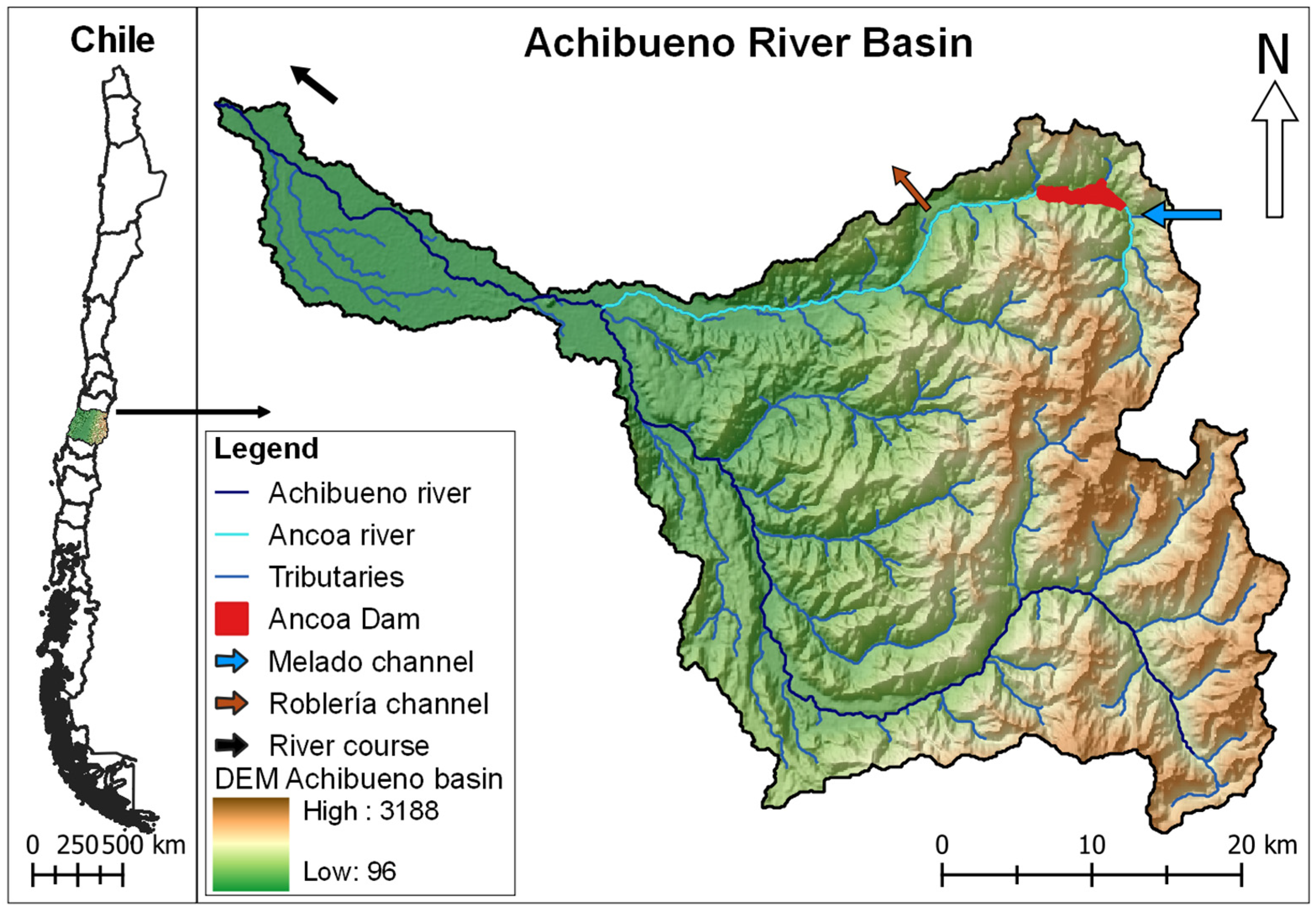
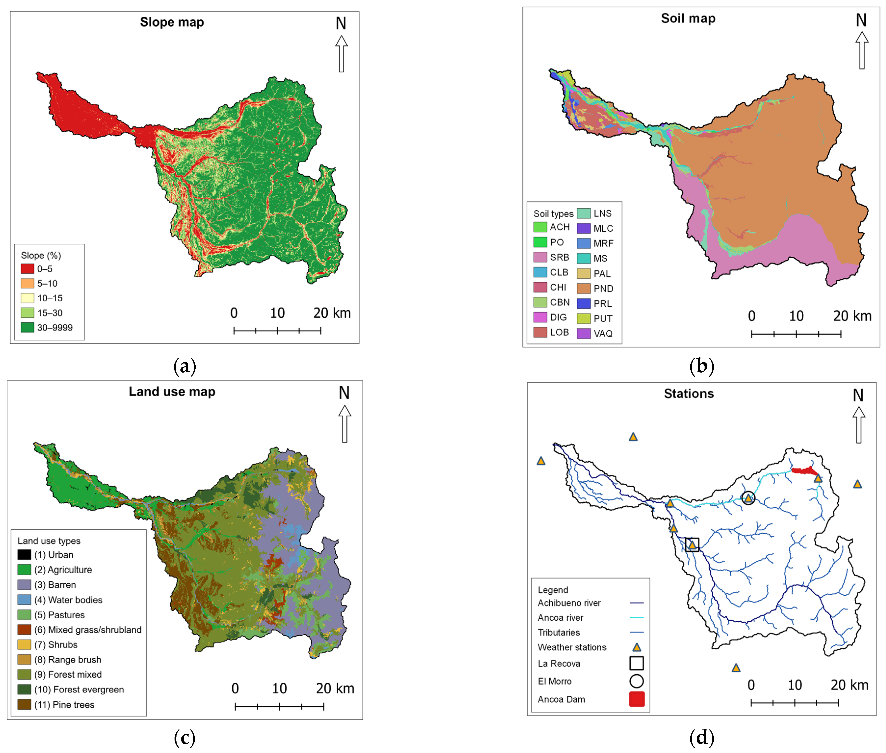
2.1. Study Area

The Achibueno River Basin is located in the Maule region, VII Region of Chile, in the coastal mountain range between 35°51′S and 71°40′W. The catchment area is 1551 km2, and the basin is a sub-basin of the mountain basin located at the Loncomilla River in southcentral Chile (Figure 1). The area is composed of intrusive rocks, sedimentary sequences, volcanic, and volcanic-sedimentary sequences [41], and the elevation ranges from 96 m to 3188 m above sea level. The area is dominated by temperate Mediterranean climatic conditions and an annual precipitation of approximately 1908 mm, with a dry southern summer precipitation level of 75 mm/year (December, January, February) and a rainy southern winter precipitation level of 1032 mm/year (June, July, August) [42].
The Ancoa Dam stores water for agricultural uses and generates electricity via a run-of-river hydroelectric power plant located at the foot of the dam. Additionally, Melado and Roblería are two inter-basin transfer channels located in the Ancoa River that were established to increase the water availability in the Ancoa, Achibueno, and Putagán Rivers in the Maule region. The Melado Channel transfers water from the Melado River, while the Roblería Channel relocates water from the Ancoa River to the Putagán River, which is located outside the watershed borderline.

2.2. SWAT+ Model Setup

The Soil and Water Assessment Tool + (SWAT+), is a semi-distributed agro-hydrological model developed to assess the impacts of land management and climate on water resources at the basin scale [26]. SWAT+ simulates several physical processes of the hydrological cycle at different time steps based on the water balance equation (Equation (1)).
S W t = S W o + i = 1 t ( P r S u r q L a t q E T P e r c )
where S W t is the final soil water content (mm), S W o is the initial soil water content (mm), t is the time step (days), P r is the amount of precipitation on day i (mm), S u r q is the amount of surface runoff on day i (mm), L a t q is the amount of lateral flow to the channel on day i (mm), E T is the amount of evapotranspiration on day i (mm), and P e r c is the amount of percolation of soil water from the bottom of the soil profile on day i (mm).
SWAT+ (v.2.3.3) was operated via QSWAT+ (v.2.4.7) on QGIS (v.3.22) [43]. The creation of river networks and natural flow paths was automatically established by QSWAT+ based on the minimum river threshold and the point of union with the Loncomilla River as a headwater stream (Figure 1). In addition, the Ancoa Dam was manually added according to area delimitation and local information. Hydrological response units (HRUs) were generated by QSWAT+ on the basis of raster images by merging the slope map from the digital elevation model (DEM), soil type map, and land use map. Meteorological forcing data at daily time steps were used for the determination of the main processes involved in catchment hydrology.

2.2.1. Input Parameters in SWAT+

The DEM was obtained by the Shuttle Radar Topography Mission (STRM) with a 90 m spatial resolution (Figure 1) [44]. The other input parameters are presented in Table 1.
The landscape slope was divided by QSWAT+ into five categories (Figure 2a) based on the information from the DEM. The soil data required to complete the input database of the model were obtained through field studies in the catchment, in addition to information obtained from Agrological Studies of the VII Region conducted by the Natural Resources Information Center (CIREN) in 1997 (Table 2). Thus, a comprehensive soil map was generated for the studied area using 17 soil types described by CIREN [45], in addition to soil samples, local observations during field studies, and soil analysis in the laboratory (Figure 2b).
Soil samples were collected to corroborate and complement the soil description from CIREN (Table 2). Soil physicochemical data such as bulk density (BD), soil carbon content (CBN), hydraulic conductivity (K), pH, and texture were collected by fieldwork in the framework of this study. The soil samples were analyzed at the Laboratory of Soils and Foliar Analysis of Pontificia Universidad Católica de Valparaíso (PUCV). The prevailing soil textures in the catchment are clay loam soils (66.0%) that originate from sedimentary deposits with moderate permeability; loamy silt soils (23.7%) that originate from basic volcanic materials; and loamy soils (2.2%) that have an alluvial origin and consist of sedimentary soils [45].
Hydro-meteorological input data at daily time steps from 1979 to 2019 were acquired from the Catchment Attributes and Meteorology for Large-sample Studies—Chile dataset (Camels-CL) [42]. In particular, nine reference stations located in the region surrounding the study area (Figure 2d) were selected for precipitation and temperature (minimum and maximum). The Explorador solar database from the Chilean Ministry of Energy was used for the solar radiation data [47]. Due to the scarcity of local data in the Achibueno River Basin and areas with a similar climate, time series of relative air humidity and wind velocity from surrounding stations of the mountain range of the Mataquito River Basin, Maule region, were supplied by the “Dirección General de Aguas” (DGA), the Central Water Directorate.
Discharge data are available for the period 1979 to 2019 from two discharge stations located in the catchment: Rio Ancoa en El Morro (lat. −35°9′S, long. −71°3′W), and Río Achibueno en La Recova (lat. −36°0′S, long. −71°4′W) [42]. However, due to some gaps in information and unreliable discharge peak values from the Rio Ancoa en El Morro station, Río Achibueno en La Recova was selected for calibration and validation procedures.

2.2.2. Sensitivity Analysis, Calibration, and Validation of the Model

A 41-year period (1979–2019) was selected in accordance with the available forcing records for simulating runoff processes at daily time steps in the Achibueno River Basin and included a one-year period for model warm-up. The Rio Ancoa en La Recova discharge station was selected as the observed reference value for the sensitivity analysis and calibration procedures from 1996 to 1998 and from 2000 to 2002 for model validation, respectively. SWAT+ Toolbox v1.0, a sensitivity and automatic calibration tool, was used for the global sensitivity analysis and calibration procedures. Sensitivity analysis was carried out based on reports in the literature [48,49] and previous experience in the region [38]. With the most sensitive parameters, 1000 iterations were performed under SWAT+ Toolbox for the calibration period from 1996 to 1998 at daily time steps. Subsequently, the model was validated for the period from 2000 to 2002 based on the availability and continuity of the discharge records.
Efficiency criteria were calculated to assess the model performance including the coefficient of determination (R2) and goodness of fit measures such as the Nash–Sutcliffe efficiency (NSE), RMSE-observation standard deviation ratio (RSR), percentage bias (PBIAS), and Kling–Gupta efficiency (KGE). The recommended ranges of values for each efficiency criterion [50,51,52,53] were evaluated during the calibration and validation periods of the model.

2.3. Climate Model Evaluation

2.3.1. Selected Climate Models

One local and three regional climate models forced under the basis of GCMs from the Fifth Phase of the Coupled Model Intercomparison Project (CMIP5), and the Coordinated Regional Climate Downscaling Experiment (CORDEX) were selected for the assessment of future climate scenarios, particularly with respect to precipitation and temperature (minimum and maximum). A local climate model from Chile with a resolution of 10 km (Local 10 k), developed by the Center of Climate and Resilience Research ((CR)2) [54], was established based on the GCM MPI-ESM-MR (Max Planck Institute for Meteorology, Hamburg, Germany), and the Regional Climate Model System version 4.6 (RegCM 4.6). A regional climate model from Chile with a 50 km resolution (Reg 50 k) was developed by (CR)2 [54] based on REMO 2009 and RegCM 4.6. The Local 10 k and Reg 50 k datasets include actual observations and atmospheric reanalysis data from CR2MET, a product for the continental Chilean territory with a 5 km spatial resolution and historical data from 1979 to 2016. In addition, time series from two RCMs from the CORDEX project were evaluated, Remo 2015 based on the GCMs MPI-ESM-LR, and RegCM 4.7 based on the GCMs MPI-ESM-MR. Both RCMs have a resolution of 0.22° (~25 km) and incorporate ERA-Interim reanalysis data from 1970 to 2005 as the historical period. Therefore, to evaluate the effect of different bias correction methods on the precipitation and temperature datasets, the historical time series from 1979 to 2005 at a daily time step was selected. For graphical displays, the empirical cumulative distribution function (ECDF) is presented to compare the historical periods without bias correction against the observed dataset.

2.3.2. Bias Correction Methods

Quantile mapping methods (QMMs) were selected for bias correction, particularly because they implement statistical transformations for the post-processing of climate modeling outputs and are recommended by researchers [15,17]. In particular, parametric transformation function (PTF), distribution derived transformation (DIST), and non-parametric transformations as empirical quantiles (QUANT), robust empirical quantiles (RQUANT), and smoothing spline (SSPLIN) were used and evaluated. The selected quantile mapping methods for bias correction were applied using the R package “Qmap” (v.1.0-4) [15] and are described as follows:
The exponential tendency to an asymptote (expasympt) method was used as the PTF and is defined as:
P o = ( a + b P m ) 1 e P m τ
where P o and P m are the probabilities of the observed and modeled variables, respectively; a , b , and τ are method-related parameters that are subject to calibration.
The DIST allows us to adjust the distribution of a modeled variable ( P m ) so that it matches the distribution of an observed variable ( P o ) . This is defined as:
P o = F m 1 F m P m
where F is a cumulative distribution function (CDF) and F 1 is the corresponding quantile function (inverse CDF). The subscripts o and m indicate the parameters of the distribution that correspond to the observed and modeled data, respectively. The DIST includes Bernoulli and Gamma distributions to compute the occurrence probability and intensities of precipitation, therefore, it is recommended only for precipitation [55].
The QUANT estimates values of the empirical CDF of the observed and modeled time series for regularly spaced quantiles. Accordingly, QUANT employs interpolation to estimate data with unavailable quantile values. RQUANT employs local linear least squares regression to estimate the values of the quantile–quantile relation of the observed and modeled time series for regularly spaced quantiles. Similarly to QUANT, unavailable quantile values are estimated by the interpolation of fitted values. In SSPLIN, a smoothing spline is fitted to the quantile–quantile plot of the observed and modeled time series.
In the case of precipitation, the PTF, DIST, QUANT, RQUANT, and SSPLIN were evaluated, while for the minimum and maximum temperatures, the PTF, QUANT, RQUANT, and SSPLIN were evaluated.

2.3.3. Evaluation of Bias Correction

The bias correction methods were evaluated using raw and bias-corrected time series from the historical period (1979–2005) of the evaluated climate models related to the observed precipitation and maximum and minimum temperature datasets at a daily time step. Statistical measures such as the mean bias error (MBE), mean absolute error (MAE), and root mean square error (RMSE) were used, and are described as follows:
M B E = n 1 i = 1 n P E i P o b s i
M A E = n 1 i = 1 n P E i P o b s i
R M S E = n 1 i = 1 n P E i P o b s i 2
where P E i is the model estimate for the involved data point i , P o b s i is the observed value for the considered data point i , and n is the length of the distribution of the data point being analyzed.
Positive and negative values from MBE indicate the underestimation and overestimation of bias, respectively, while zero values indicate an absence of bias in the generated results. In the case of MAE and RMSE, both methods only have positive values, where 0 values indicates a perfect match between the observed and corrected values [56].

2.3.4. Climate Scenarios

After the implementation of the most effective bias correction method on the evaluated climate models, future climate scenarios based on Representative Concentration Pathways (RCPs) 2.6 and 8.5 were used as the forcing input data for the period from 2025 to 2050 in the calibrated and validated SWAT+ model. In addition, the effect of climate scenarios on the hydrological response of the Achibueno River Basin were evaluated. For the graphical displays, the impacts of future climate scenarios on the water balance components and surface runoff are presented.

3. Results

3.1. Swat+ Simulation, Calibration, and Validation

The simulation of a 41-year period (1979 to 2019) was successfully performed with SWAT+, which included a total of 21 sub-basins, 211 channels, and 5390 HRUs. In relation to the sensitivity analysis, seven parameters were selected due to their significant effects on the modeled runoff in the Achibueno River Basin. After the calibration process had been completed, the efficiency criteria were calculated for the calibration and validation periods (Table 3).
Satisfactory model performances were obtained with an NSE of 0.58 and 0.65 for the calibration and validation periods, respectively. Under the recommended ranges of values [52], the NSE at the daily time step can be considered satisfactory when the NSE values are greater than 0.50. R2 values were considered good and improved from 0.44 in the simulation to 0.69, and 0.67 for the calibration and validation periods, respectively. RSR ranged from 1.15 to 0.64 during calibration and 0.59 during validation; therefore, the model performances were considered satisfactory and good, respectively. The PBIAS values were classified as very good for the simulation and calibration periods (4.9% and 1.5%, respectively), while for the validation period, they were classified as good (−14.5%). The variation in PBIAS during the validation period was associated with a bias in the discharge peaks difficult to achieve. Similar observations for PBIAS have been presented in previous studies based on daily time steps in the region [38]. In addition, the KGE improved from unsatisfactory to very good with values ranging from 0.36 to 0.77 during the calibration period and was classified as good during the validation period, with a value of 0.74. Even when the NSE and KGE values cannot be directly compared because their relationships are non-unique and have a partial dependency on the coefficient of variation from the observed time series [50], both statistics provide relevant information for use in the calibration and validation procedures, especially in areas where data are scare.

3.2. Climate Models

The empirical cumulative distribution function (ECDF) during the historical period (1979–2005) from the Camels-CL dataset and the evaluated climate models without bias correction are presented for the precipitation (Figure 3), minimum temperature (Tmin) (Figure 4), and maximum temperature (Tmax) (Figure 5). In addition, the range of values from the Camels-CL dataset and the evaluated climate models during the historical period (1979–2005) without bias correction are presented in Table 4.
For the historical period from the Camels-CL dataset, the precipitation ranged from 0 to 203 mm/day as the maximum precipitation, obtained from the hydro-meteorological station of Rio Ancoa Antes Tunel Canal Melado (Figure 3c). In the case of the evaluated climate model, the maximum precipitation values were obtained at Rio Acoa en El Morro (Figure 3e), located in the middle part of the Achibueno Basin, together to Rio Ancoa Antes Tunel Canal Melado (Figure 3c) and Rio Melado en El Salto (Figure 3h), both hydro-meteorological stations located in the upper part of the basin. It is known that RCM outputs can present bias related to coarse-resolution, especially in complex areas with strong surface forcing like the Andes Mountains [57], in addition to the scarce presence of hydro-meteorological stations [58]. The Achibueno Basin is located in the mountainous areas of the Maule region, thus, as the data suggest, the evaluated climate models clearly overestimated the precipitation values, and a similar observation has been reported for other RCMs in South America [58,59].
In the case of minimum temperature, Rio Melado en El Salto (Figure 4h) presented the lowest temperature record during the historical period from the Camels-CL dataset with −14.1 °C. Rio Putagan en Yerbas Buenas (Figure 4i) was the station with the highest minimum temperature value of 15.8 °C. However, in the evaluated climate models, Rio Putagan en Yerbas Buenas presented the lowest temperature, particularly under RegCM 4.7 with −44.1 °C. In addition, Rio Loncomilla en Bodega (Figure 4f) presented the highest values of minimum temperature, in particular under Remo 2015 with 24.4 °C.
Similar to the minimum temperatures, Rio Melado en El Salto (Figure 5h) presented the lowest maximum temperature record during the historical period from the Camels-CL dataset with −5.7 °C. In addition, Rio Putagan en Yerbas Buenas (Figure 5i) station had the highest maximum temperature value in the Camels-CL dataset with 34.1 °C. However, in the evaluated climate models, the referential station Putagan en Yerbas Buenas presented the lowest temperature, particularly under RegCM 4.7 with −13.2 °C. In addition, Rio Loncomilla en Bodega (Figure 5f) presented the highest value of maximum temperature, particularly under RegCM 4.7 with 44.2 °C. In the case of both the minimum and maximum temperatures, the evaluated climate models under- and overestimated the temperatures, similar to López-Franca et al. [60]. Although the Local 10 k and Reg 50 k include actual observations and atmospheric reanalysis data during the historical period, both climate models presented bias with relation to the Camels-CL dataset. Therefore, in order to avoid confusing or erroneous results from the evaluated climate models related to the overestimation of precipitation and the under- and overestimation of the temperature, bias correction methods were implemented before the evaluation of future climate scenarios in the Achibueno River Basin.

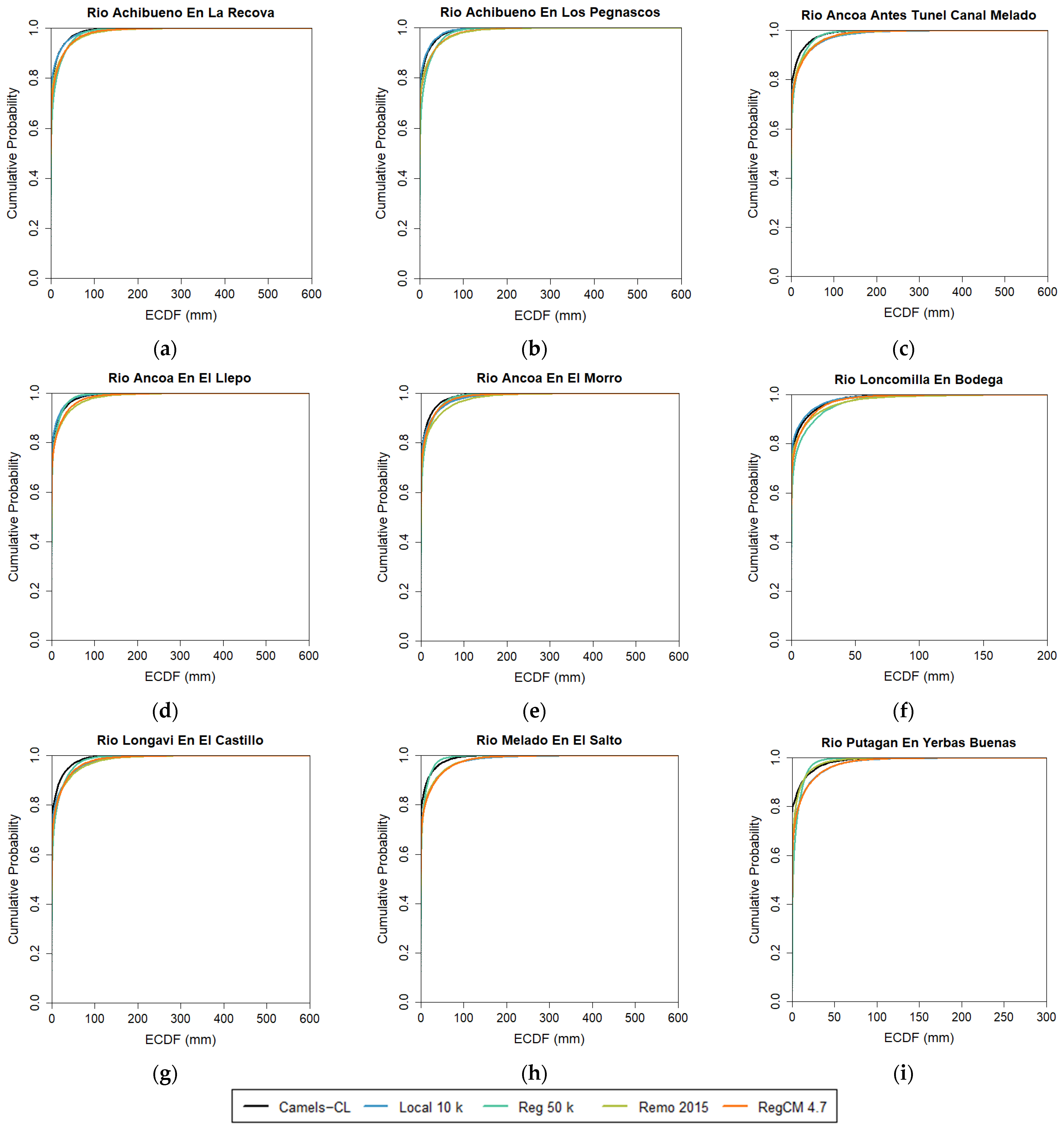
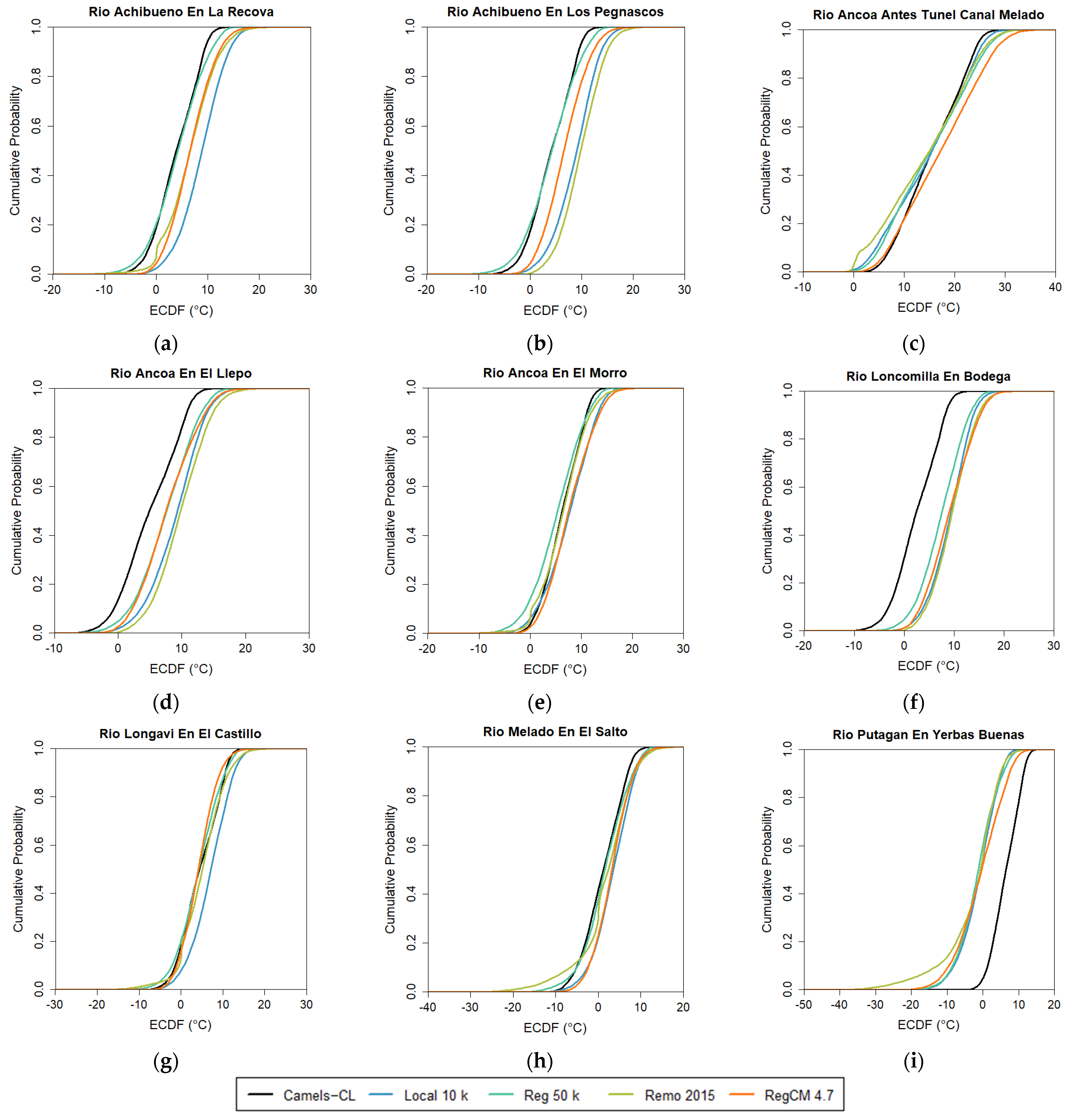
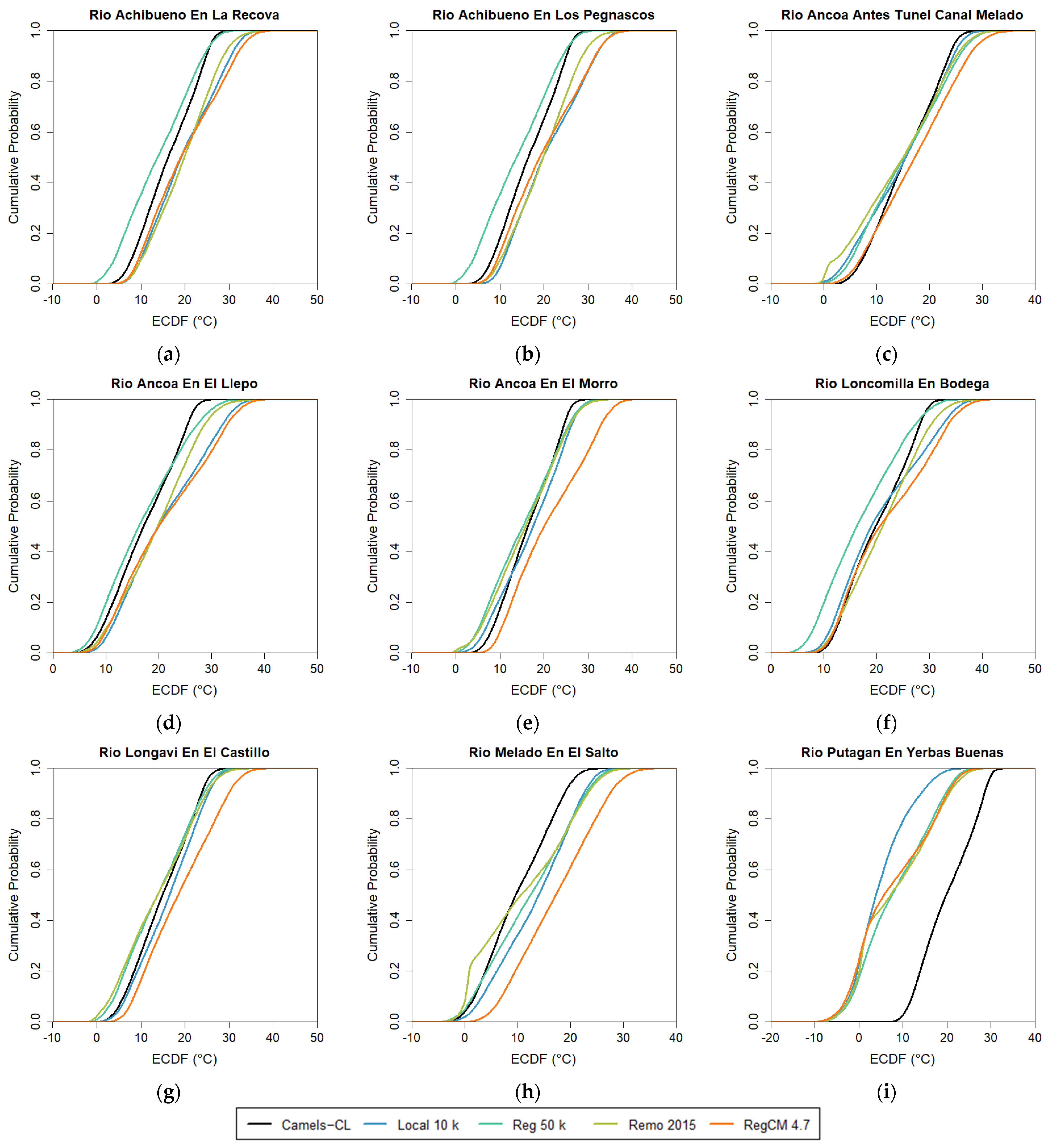
3.3. Bias Correction Methods

Quantile mapping methods were evaluated on the historical period (1979–2005) of the climate models, taking as reference the hydro-meteorological stations and observed data from the Camels-CL dataset. For precipitation, the PTF, DIST, QUANT, RQUANT, and SSPLIN were applied. In addition, the PTF, QUANT, RQUANT, and SSPLIN were implemented for minimum and maximum temperatures. In order to compare the bias correction methods in the four evaluated climate models, the MBE, MAE, and RMSE were calculated for the precipitation, minimum temperature (Tmin), and maximum temperature (Tmax), respectively (Table 5).
The comparisons of different statistical measures based on the observed values and the evaluated climate models revealed differences before and after the bias correction methods. While DIST is only recommended for precipitation [55], in this case, it was the worst accuracy bias correction method for precipitation out of the evaluated climate models, similar to the observations of other authors [17]. In the case of the PTF, QUANT, RQUANT, and SSPLIN, the MBE was satisfactory for precipitation (close to 0). However, PTF obtained a better accuracy considering the three statistical measures. In the case of temperature, although the PTF seemed promising, positive and negative values were estimated for the MBE, indicating the under- and overestimation of bias. In addition, the MAE and RMSE were the highest from the evaluated bias correction methods for temperature. In the case of SSPLIN, negative values for MBE were calculated (overestimation of the bias) even though there were similar values of MAE and RMSE compared to the other methods, similar to other authors [17]. In the case of QUANT and RQUANT, both methods indicated the best accuracy for temperature in the evaluated climate models. Moreover, the values between the reference quantiles were interpolated through linear function in QUANT, while RQUANT extended the QUANT method by using local linear least squares regression to estimate the values of the quantile–quantile relation of the modeled and observed time series [61,62,63]. Therefore, based on the higher capability to correct the modeled empirical CDF at higher percentiles [63], RQUANT seems to be more promising as a bias correction method for temperature. As a consequence, PTF was selected as the bias correction method for precipitation, and RQUANT was selected for the minimum and maximum temperatures.

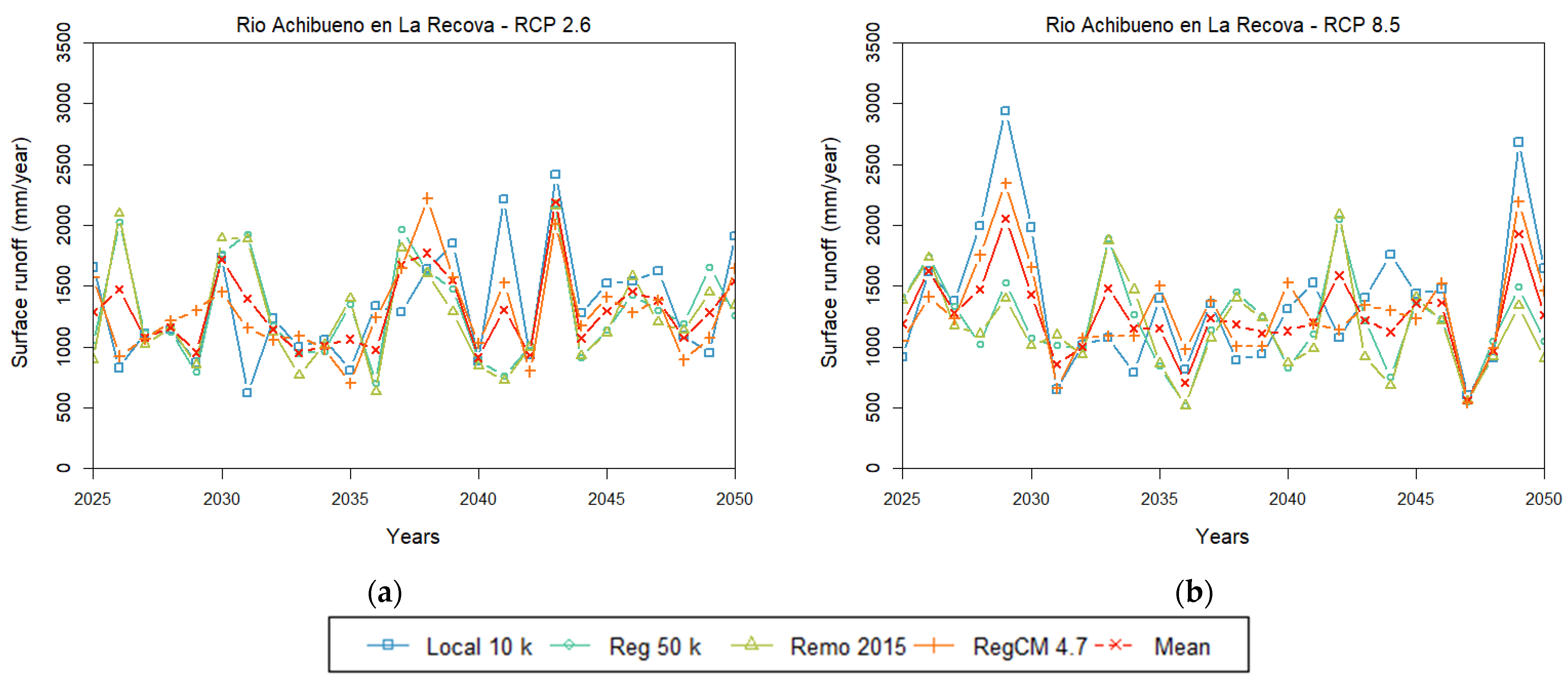
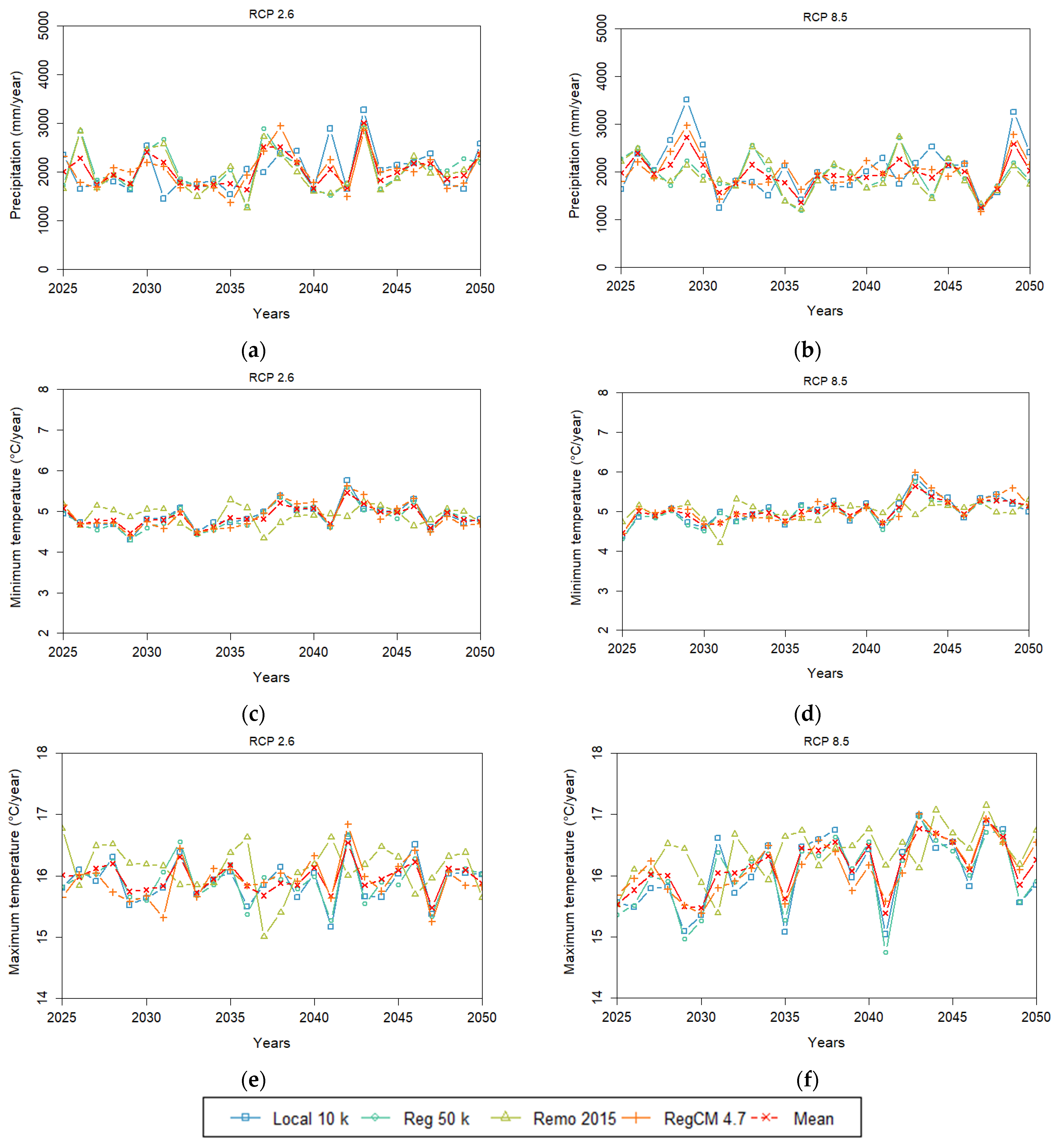
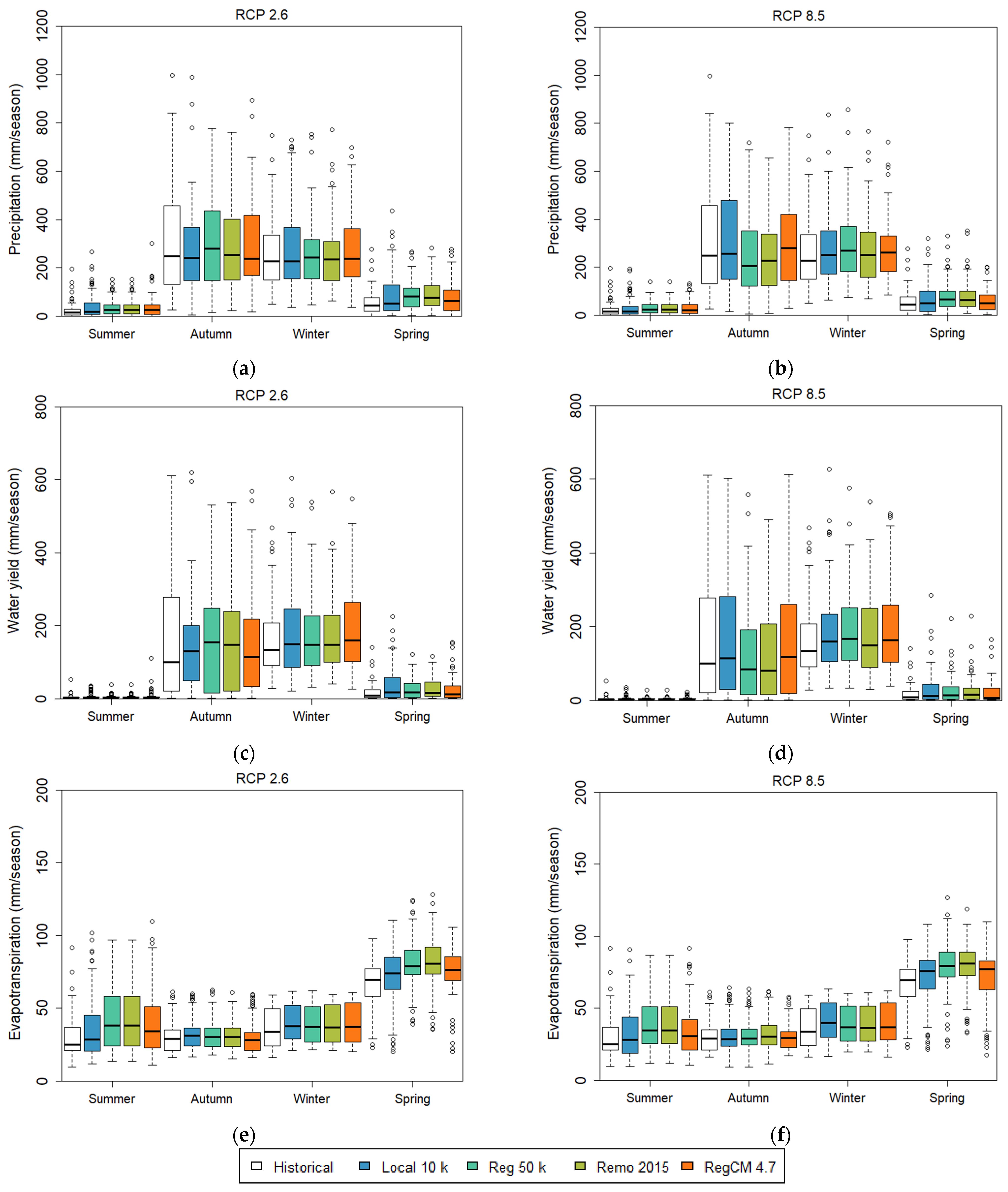
3.4. Future Climate Scenarios

After the selection of the most promising bias correction method for precipitation (PTF) and the minimum and maximum temperatures (RQUANT), bias-corrected future climate scenarios at daily time steps were generated (2025–2050) under RCPs 2.6 and 8.5 for precipitation and the minimum and maximum temperatures, respectively (Figure 6). The effects of bias-corrected future climate scenarios on the catchment hydrology components of the Achibueno River Basin under RCPs 2.6 and 8.5 are presented in Table 6, and under seasonal basis in Figure 7. In addition, projections of surface runoff at Rio Ancoa en La Recova station are presented in Figure 8.
Both the RCP 2.6 and RCP 8.5 scenarios suggest fluctuations in precipitation and temperature. The frequency and amount of precipitation in both scenarios were not homogeneous and presented strong peaks of precipitation in different periods (Figure 6a,b). In the case of maximum temperature, strong fluctuations with a tendency to increase over the years are expected to occur (Figure 6f). It is known that the effects of climate change has been severe in Chile, in particular, related to the mega-drought that has affected some regions of the country since 2010 [5,64]. Therefore, in order to compare the effects of climate change scenarios on the hydrological response of the Achibueno River Basin, a historical period of 20 years (1990–2009) under the Camels-CL dataset was used as the reference (Table 6).
Compared with the 20-year historical period, the effects of the climate scenarios on the components of the catchment hydrology reflected variations in all of the components. In particular, variations in the trends of precipitation and water yield are projected, especially for the winter and spring seasons. In addition, increases in evapotranspiration during the spring and summer seasons are projected in both scenarios (Figure 7e,f).
Differences between the evaluated climate models under the two RCP’s are projected in the hydrological response of the studied catchment. In comparison to the historical period, the four evaluated climate models suggest increases in precipitation, Latq, water yield, ET, and GW recharge under RCP 2.6. In the case of RCP 8.5, the Local 10 k and RegCM 4.7 climate models presented increases in precipitation, Latq, water yield, ET, and GW recharge compared to the historical period. In addition, the Reg 50 k and Remo 2015 climate models suggest a clear reduction in precipitation, with impacts on water fluxes and the internal moisture distribution in the catchment. Additionally, events with different intensities and amounts of precipitation are expected during short periods of time. In the case of ET, the results suggest increases in the four evaluated climate models compared to the historical period under both RCPs, mainly related to increases in temperature. Although the Local 10 k climate model was developed under the basis of RegCM 4.6, a previous version of RegCM 4.7, it is possible to observe some similarities in the trends among both climate models. In the case of Reg 50 k, a climate model developed under the basis of based Remo 2009 and RegCM 4.6, similarities were not evident in comparison to Remo 2015, especially under RCP 8.5.
The projected results of surface runoff at Rio Achibueno en La Recova station presented variations following the hydrological response of the catchment under both RCPs. In the case of RCP 2.6 (Figure 8a), the projected surface runoff presented fluctuations over the period 2025–2050 including years with a reduced amount of surface runoff but also periods with extreme values. In the case of RCP 8.5 (Figure 8b), in both the Local 10 k and RegCM 4.7 climate models, higher precipitation values were obtained under RCP 8.5, and similarly in the projected surface runoff at Rio Achibueno en La Recova station. In contrast, under the Reg 50 k and Remo 2015 climate models, a clear reduction in precipitation is expected under RCP 8.5, consequently, decreases in surface runoff were projected. However, for the overall precipitation values under RCP 8.5, it is clear that there is a tendency for a reduction in the frequency of events. Additionally, events with different intensities and amounts of precipitation are expected during short periods under both RCPs. It is known that among the effects of climate change at the basin scale, water-related problems include water scarcity under decreases in precipitation, but also potential flooding situations in cases of extreme precipitation events [65]. In addition, under both RCPs, the results suggest increases in temperature and evapotranspiration, which can contribute to an increase in the water demand for irrigation. Therefore, it is important to consider the current and future management practices related to the protection of water resources in order to prevent both situations: possible increases in flooding under extreme precipitation events, and increases in the water demand for irrigation under reduced precipitation periods.
Although bias correction methods can be implemented in the different outputs of RCMs like precipitation and temperature, some authors recommend the bias correction of surface runoff in order to assess the impact of climate change at the basin scale under a scarcity of observed precipitation and temperature time series [66]. However, it is known that RCMs can increase the biases related to precipitation and/or temperature under certain conditions like warmer or wetter climatic conditions [67]. Even when there are different bias correction methods, a proper bias correction method should consider a case-by-case implementation based on the availability of hydro-meteorological records and the local conditions. For instance, in mountainous areas, some physical limitations can contribute to random biases in the surrounding mountain ranges [9]. Because of the local conditions in the Achibueno River Basin, and based on the presented results, we encourage the use of quantile mapping like PTF and RQUANT as bias correction methods in studies focused on assessing the climate change impacts at the basin scale, in order to avoid the under- or overestimation of precipitation and temperature, especially in mountainous areas. Thus, we recommend maintaining efforts in preserving the hydro-meteorological networks, especially in mountainous areas, in order to reduce bias-related uncertainties and in the prevention of flooding events related to extreme precipitation. The combined effect of bias-corrected future climate scenarios and future land use change under different management practices in the region is a matter of ongoing research.

4. Conclusions

We present the evaluation of five bias correction methods and the effects of bias-corrected future climate scenarios on the hydrological response of the Achibueno River Basin in southcentral Chile. Quantile mapping methods were evaluated for precipitation and temperature (maximum and minimum) in the historical period (1979–2005) of one local climate model and three regional climate models. Parametric transformation function (PTF) and robust empirical quantile (RQUANT) were the most prominent bias correction methods for precipitation and temperature, respectively. The effects of bias-corrected future climate scenarios based on Representative Concentration Pathways (RCPs) 2.6 and 8.5 from the four climate models were evaluated over the period 2025–2050 on the hydrological response of the Achibueno River Basin by simulating hydrological fluxes with SWAT+ at daily time steps. Bias-corrected future climate scenarios resulted in differences in precipitation and temperature under both RCP scenarios. In the case of RCP 2.6, an increase in precipitation, water yield, evapotranspiration, and groundwater recharge were projected for all the evaluated climate models. In contrast, under RCP 8.5, strong peaks of precipitation in different periods, with differences in amount as well as frequency, were projected, especially under the Local 10 k and RegCM 4.7 climate models scenarios. As a consequence, variation in the overall water yield, increases in evapotranspiration, and partial decreases in groundwater recharge were projected. In this regard, yearly fluctuations in surface runoff under RCP 2.6 were projected, while for RCP 8.5, strong peaks in short periods of time together with decreases in surface runoff were projected. In both scenarios, the most promising and also the most impacting changes in catchment hydrology attributable to the fluctuation in precipitation and surface runoff with simultaneous increases in evapotranspiration are expected to occur, with clear impacts on future water availability. Consequently, increases in flood events under extreme precipitation as well as increases in the water demand for irrigation under reduced precipitation periods are changes that most likely will take place. Therefore, it is important to consider possible adaptation strategies of current and future river basin management practices in the interest of protecting water resources in the mountainous areas of southcentral Chile.

Author Contributions

Conceptualization, H.M., I.A. and P.R.; Methodology, H.M.; Software, H.M.; Validation, H.M. and I.A.; Formal analysis, H.M.; Investigation, H.M.; Resources, H.M., I.A. and P.R.; Data curation, H.M.; Writing-original draft preparation, H.M.; Writing-review and editing, H.M., I.A., J.L.C.-D., C.H.-P. and P.R.; Visualization, H.M.; Supervision, I.A., J.L.C.-D., C.H.-P. and P.R.; Project administration, I.A. and P.R.; Funding acquisition, I.A., J.L.C.-D., C.H.-P. and P.R. All authors have read and agreed to the published version of the manuscript.

Funding

This research was funded by Bundesministerium für Bildung und Forschung (BMBF), Project no. 01DN17041. In addition, this work was partially funded by ANID/CERES/R23F0002-R23F0003.

Data Availability Statement

The data presented in this study are available on request from the corresponding author.

Acknowledgments

We acknowledge Bundesministerium für Bildung und Forschung (BMBF) for financial support through Grant no. 01DN17041. The authors are also grateful to the Laboratory of Soil and Foliar Analysis of Pontificia Universidad Católica de Valparaíso (PUCV) for its support in performing the soil sample analysis for the Achibueno River Basin. In addition, the authors are also grateful to Regional Center CERES. JLCD is supported by ANID BASAL/FB210006 and is an associated researcher to the Centro de Acción Climática-PUCV.

Conflicts of Interest

The authors declare no conflicts of interest. The financial support agencies had no role in the design of the study; in the collection, analyses, or interpretation of the data; in the writing of the manuscript; or in the decision to publish the results.

References

  1. Painter, J.; Ettinger, J.; Doutreix, M.-N.; Strauß, N.; Wonneberger, A.; Walton, P. Is it climate change? Coverage by online news sites of the 2019 European summer heatwaves in France, Germany, the Netherlands, and the UK. Clim. Chang. 2021, 169, 4. [Google Scholar] [CrossRef]
  2. Nissen, K.M.; Ulbrich, U. Increasing frequencies and changing characteristics of heavy precipitation events threatening infrastructure in Europe under climate change. Nat. Hazards Earth Syst. Sci. 2017, 17, 1177–1190. [Google Scholar] [CrossRef]
  3. Lv, X.; Zuo, Z.; Ni, Y.; Sun, J.; Wang, H. The effects of climate and catchment characteristic change on streamflow in a typical tributary of the Yellow River. Sci. Rep. 2019, 9, 14535. [Google Scholar] [CrossRef] [PubMed]
  4. Moraga, J.S.; Peleg, N.; Fatichi, S.; Molnar, P.; Burlando, P. Revealing the impacts of climate change on mountainous catchments through high-resolution modelling. J. Hydrol. 2021, 603, 126806. [Google Scholar] [CrossRef]
  5. Muñoz, A.A.; Klock-Barría, K.; Alvarez-Garreton, C.; Aguilera-Betti, I.; González-Reyes, Á.; Lastra, J.A.; Chávez, R.O.; Barría, P.; Christie, D.; Rojas-Badilla, M.; et al. Water Crisis in Petorca Basin, Chile: The Combined Effects of a Mega-Drought and Water Management. Water 2020, 12, 648. [Google Scholar] [CrossRef]
  6. Neupane, D.; Adhikari, P.; Bhattarai, D.; Rana, B.; Ahmed, Z.; Sharma, U.; Adhikari, D. Does Climate Change Affect the Yield of the Top Three Cereals and Food Security in the World? Earth 2022, 3, 45–71. [Google Scholar] [CrossRef]
  7. Schmidhuber, J.; Tubiello, F.N. Global food security under climate change. Proc. Natl. Acad. Sci. USA 2007, 104, 19703–19708. [Google Scholar] [CrossRef] [PubMed]
  8. Teutschbein, C.; Seibert, J. Regional Climate Models for Hydrological Impact Studies at the Catchment Scale: A Review of Recent Modeling Strategies. Geogr. Compass 2010, 4, 834–860. [Google Scholar] [CrossRef]
  9. Cardell, M.F.; Romero, R.; Amengual, A.; Homar, V.; Ramis, C. A quantile–quantile adjustment of the EURO-CORDEX projections for temperatures and precipitation. Int. J. Climatol. 2019, 39, 2901–2918. [Google Scholar] [CrossRef]
  10. Chen, J.; Arsenault, R.; Brissette, F.P.; Zhang, S.B. Climate Change Impact Studies: Should We Bias Correct Climate Model Outputs or Post-Process Impact Model Outputs? Water Resour. Res. 2021, 57, e2020WR028638. [Google Scholar] [CrossRef]
  11. Gumindoga, W.; Rientjes, T.H.M.; Tamiru Haile, A.; Makurira, H.; Reggiani, P. Performance of bias-correction schemes for CMORPH rainfall estimates in the Zambezi River basin. Hydrol. Earth Syst. Sci. 2019, 23, 2915–2938. [Google Scholar] [CrossRef]
  12. Holthuijzen, M.; Beckage, B.; Clemins, P.J.; Higdon, D.; Winter, J.M. Robust bias-correction of precipitation extremes using a novel hybrid empirical quantile-mapping method: Advantages of a linear correction for extremes. Theor. Appl. Climatol. 2022, 149, 863–882. [Google Scholar] [CrossRef]
  13. Maraun, D. Bias Correcting Climate Change Simulations—A Critical Review. Curr. Clim. Chang. Rep. 2016, 2, 211–220. [Google Scholar] [CrossRef]
  14. Ngai, S.T.; Tangang, F.; Juneng, L. Bias correction of global and regional simulated daily precipitation and surface mean temperature over Southeast Asia using quantile mapping method. Glob. Planet. Chang. 2017, 149, 79–90. [Google Scholar] [CrossRef]
  15. Gudmundsson, L.; Bremnes, J.B.; Haugen, J.E.; Engen-Skaugen, T. Technical Note: Downscaling RCM precipitation to the station scale using statistical transformations; a comparison of methods. Hydrol. Earth Syst. Sci. 2012, 16, 3383–3390. [Google Scholar] [CrossRef]
  16. Ayugi, B.; Tan, G.; Ruoyun, N.; Babaousmail, H.; Ojara, M.; Wido, H.; Mumo, L.; Ngoma, N.H.; Nooni, I.K.; Ongoma, V. Quantile Mapping Bias Correction on Rossby Centre Regional Climate Models for Precipitation Analysis over Kenya, East Africa. Water 2020, 12, 801. [Google Scholar] [CrossRef]
  17. Enayati, M.; Bozorg-Haddad, O.; Bazrafshan, J.; Hejabi, S.; Chu, X.F. Bias correction capabilities of quantile mapping methods for rainfall and temperature variables. J. Water Clim. Chang. 2021, 12, 401–419. [Google Scholar] [CrossRef]
  18. Soriano, E.; Mediero, L.; Garijo, C. Selection of Bias Correction Methods to Assess the Impact of Climate Change on Flood Frequency Curves. Water 2019, 11, 2266. [Google Scholar] [CrossRef]
  19. Sundaram, G.; Radhakrishnan, S. Performance Evaluation of Bias Correction Methods and Projection of Future Precipitation Changes Using Regional Climate Model over Thanjavur, Tamil Nadu, India. Ksce J. Civ. Eng. 2023, 27, 878–889. [Google Scholar] [CrossRef]
  20. Breuer, L.; Huisman, J.A.; Willems, P.; Bormann, H.; Bronstert, A.; Croke, B.F.W.; Frede, H.G.; Graff, T.; Hubrechts, L.; Jakeman, A.J.; et al. Assessing the impact of land use change on hydrology by ensemble modeling (LUCHEM). I: Model intercomparison with current land use. Adv. Water Resour. 2009, 32, 129–146. [Google Scholar] [CrossRef]
  21. Dwarakish, G.S.; Ganasri, B.P.; De Stefano, L. Impact of land use change on hydrological systems: A review of current modeling approaches. Cogent Geosci. 2015, 1, 1115691. [Google Scholar] [CrossRef]
  22. Klöcking, B.; Ströbl, B.; Knoblauch, S.; Maier, U.; Pfützner, B.; Gericke, A. Development and allocation of land-use scenarios in agriculture for hydrological impact studies. Phys. Chem. Earth Parts A/B/C 2003, 28, 1311–1321. [Google Scholar] [CrossRef]
  23. Lahmer, W.; Pfutzner, B.; Becker, A. Assessment of land use and climate change impacts on the mesoscale. Phys. Chem. Earth Part B-Hydrol. Ocean. Atmos. 2001, 26, 565–575. [Google Scholar] [CrossRef]
  24. Arnold, J.G.; Srinivasan, R.; Muttiah, R.S.; Williams, J.R. Large Area Hydrologic Modeling and Assessment Part I: Model Development1. JAWRA J. Am. Water Resour. Assoc. 2007, 34, 73–89. [Google Scholar] [CrossRef]
  25. Bieger, K.; Arnold, J.G.; Rathjens, H.; White, M.J.; Bosch, D.D.; Allen, P.M. Representing the Connectivity of Upland Areas to Floodplains and Streams in SWAT. J. Am. Water Resour. Assoc. 2019, 55, 578–590. [Google Scholar] [CrossRef]
  26. Bieger, K.; Arnold, J.G.; Rathjens, H.; White, M.J.; Bosch, D.D.; Allen, P.M.; Volk, M.; Srinivasan, R. Introduction to SWAT plus, A Completely Restructured Version of the Soil and Water Assessment Tool. J. Am. Water Resour. Assoc. 2017, 53, 115–130. [Google Scholar] [CrossRef]
  27. Musie, M.; Sen, S.; Chaubey, I. Hydrologic Responses to Climate Variability and Human Activities in Lake Ziway Basin, Ethiopia. Water 2020, 12, 164. [Google Scholar] [CrossRef]
  28. Nasiri, S.; Ansari, H.; Ziaei, A.N. Simulation of water balance equation components using SWAT model in Samalqan Watershed (Iran). Arab. J. Geosci. 2020, 13, 421. [Google Scholar] [CrossRef]
  29. Nkwasa, A.; Chawanda, C.J.; Msigwa, A.; Komakech, H.C.; Verbeiren, B.; van Griensven, A. How Can We Represent Seasonal Land Use Dynamics in SWAT and SWAT plus Models for African Cultivated Catchments? Water 2020, 12, 1541. [Google Scholar] [CrossRef]
  30. Araya-Osses, D.; Casanueva, A.; Román-Figueroa, C.; Uribe, J.M.; Paneque, M. Climate change projections of temperature and precipitation in Chile based on statistical downscaling. Clim. Dyn. 2020, 54, 4309–4330. [Google Scholar] [CrossRef]
  31. Blin, N.; Hausner, M.; Leray, S.; Lowry, C.; Suarez, F. Potential impacts of climate change on an aquifer in the arid Altiplano, northern Chile: The case of the protected wetlands of the Salar del Huasco basin. J. Hydrol.-Reg. Stud. 2022, 39, 100996. [Google Scholar] [CrossRef]
  32. Martínez-Retureta, R.; Aguayo, M.; Stehr, A.; Sauvage, S.; Echeverría, C.; Sánchez-Pérez, J.-M. Effect of Land Use/Cover Change on the Hydrological Response of a Southern Center Basin of Chile. Water 2020, 12, 302. [Google Scholar] [CrossRef]
  33. Omani, N.; Srinivasan, R.; Karthikeyan, R.; Reddy, K.V.; Smith, P.K. Impacts of Climate Change on the Glacier Melt Runoff from Five River Basins. Trans. Asabe 2016, 59, 829–848. [Google Scholar] [CrossRef]
  34. Omani, N.; Srinivasan, R.; Karthikeyan, R.; Smith, P.K. Hydrological Modeling of Highly Glacierized Basins (Andes, Alps, and Central Asia). Water 2017, 9, 111. [Google Scholar] [CrossRef]
  35. Stehr, A.; Debels, P.; Arumi, J.L.; Romero, F.; Alcayaga, H. Combining the Soil and Water Assessment Tool (SWAT) and MODIS imagery to estimate monthly flows in a data-scarce Chilean Andean basin. Hydrol. Sci. J.-J. Des Sci. Hydrol. 2009, 54, 1053–1067. [Google Scholar] [CrossRef]
  36. Stehr, A.; Debels, P.; Romero, F.; Alcayaga, H. Hydrological modelling with SWAT under conditions of limited data availability: Evaluation of results from a Chilean case study. Hydrol. Sci. J.-J. Des Sci. Hydrol. 2008, 53, 588–601. [Google Scholar] [CrossRef]
  37. Martínez Martínez, Y.; Goecke Coll, D.; Aguayo, M.; Casas-Ledón, Y. Effects of landcover changes on net primary production (NPP)-based exergy in south-central of Chile. Appl. Geogr. 2019, 113, 102101. [Google Scholar] [CrossRef]
  38. Moya, H.; Althoff, I.; Huenchuleo, C.; Reggiani, P. Influence of Land Use Changes on the Longaví Catchment Hydrology in South-Center Chile. Hydrology 2022, 9, 169. [Google Scholar] [CrossRef]
  39. Stehr, A.; Aguayo, M.; Link, O.; Parra, O.; Romero, F.; Alcayaga, H. Modelling the hydrologic response of a mesoscale Andean watershed to changes in land use patterns for environmental planning. Hydrol. Earth Syst. Sci. 2010, 14, 1963–1977. [Google Scholar] [CrossRef]
  40. Uniyal, B.; Dietrich, J.; Vu, N.Q.; Jha, M.K.; Arumi, J.L. Simulation of regional irrigation requirement with SWAT in different agro-climatic zones driven by observed climate and two reanalysis datasets. Sci. Total Environ. 2019, 649, 846–865. [Google Scholar] [CrossRef]
  41. SERNAGEOMIN. Mapa Geológico de Chile: Versión digital; Publicación Geológica Digital, No. 4. 2003. Available online: http://www.ipgp.fr/~dechabal/Geol-millon.pdf (accessed on 12 February 2024).
  42. Alvarez-Garreton, C.; Mendoza, P.A.; Boisier, J.P.; Addor, N.; Galleguillos, M.; Zambrano-Bigiarini, M.; Lara, A.; Puelma, C.; Cortes, G.; Garreaud, R.; et al. The CAMELS-CL dataset: Catchment attributes and meteorology for large sample studies—Chile dataset. Hydrol. Earth Syst. Sci. 2018, 22, 5817–5846. [Google Scholar] [CrossRef]
  43. Dile, Y.; Srinivasan, R.; George, C. QGIS Interface for SWAT+: QSWAT+. 2022 (v 2.0). Available online: http://docplayer.net/204909159-Qgis-interface-for-swat-qswat.html (accessed on 12 February 2024).
  44. Jarvis, A.; Reuter, H.I.; Nelson, A.; Guevara, E. Hole-Filled Seamless SRTM Data V4, International Centre for Tropical Agriculture (CIAT). CIAT. 2008. Available online: http://srtm.csi.cgiar.org (accessed on 12 February 2024).
  45. CIREN. Estudio Agrológico VII Región. Descripción de Suelos, Materiales y Símbolos; Centro de Información de Recursos Naturales: Santiago, Chile, 1997; pp. 1–660. [Google Scholar]
  46. CONAF. Catastro de Uso del Suelo y Vegetación. Monitoreo y Actualización en la VII Región del Maule. Corporacion Nacional Forestal. 2016. Available online: http://sit.conaf.cl (accessed on 12 February 2024).
  47. Molina, A.; Falvey, M.; Rondanelli, R. A solar radiation database for Chile. Sci. Rep. 2017, 7, 14823. [Google Scholar] [CrossRef] [PubMed]
  48. Abbaspour, K.; Vaghefi, S.; Srinivasan, R. A Guideline for Successful Calibration and Uncertainty Analysis for Soil and Water Assessment: A Review of Papers from the 2016 International SWAT Conference. Water 2017, 10, 6. [Google Scholar] [CrossRef]
  49. Yen, H.; Park, S.; Arnold, J.G.; Srinivasan, R.; Chawanda, C.J.; Wang, R.Y.; Feng, Q.Y.; Wu, J.W.; Miao, C.Y.; Bieger, K.; et al. IPEAT plus: A Built-In Optimization and Automatic Calibration Tool of SWAT. Water 2019, 11, 1681. [Google Scholar] [CrossRef]
  50. Knoben, W.J.M.; Freer, J.E.; Woods, R.A. Technical note: Inherent benchmark or not? Comparing Nash--Sutcliffe and Kling--Gupta efficiency scores. Hydrol. Earth Syst. Sci. 2019, 23, 4323–4331. [Google Scholar] [CrossRef]
  51. Krause, P.; Boyle, D.P.; Bäse, F. Comparison of different efficiency criteria for hydrological model assessment. Adv. Geosci. 2005, 5, 89–97. [Google Scholar] [CrossRef]
  52. Moriasi, D.N.; Gitau, M.W.; Pai, N.; Daggupati, P. Hydrologic and Water Quality Models: Performance Measures and Evaluation Criteria. Trans. Asabe 2015, 58, 1763–1785. [Google Scholar] [CrossRef]
  53. Pool, S.; Vis, M.; Seibert, J. Evaluating model performance: Towards a non-parametric variant of the Kling-Gupta efficiency. Hydrol. Sci. J.-J. Des Sci. Hydrol. 2018, 63, 1941–1953. [Google Scholar] [CrossRef]
  54. Centro de Ciencia del Clima y la Resiliencia (CR)2. Simulaciones Climáticas Regionales. 2018. Available online: https://www.cr2.cl/wp-content/uploads/2020/05/Guia_para-la-Plataforma-de-visualizacion-de-simulaciones-clima%CC%81ticas.pdf (accessed on 12 February 2024).
  55. Ines, A.V.M.; Hansen, J.W. Bias correction of daily GCM rainfall for crop simulation studies. Agr. For. Meteorol. 2006, 138, 44–53. [Google Scholar] [CrossRef]
  56. Geleta, C.D.; Gobosho, L. Climate Change Induced Temperature Prediction and Bias Correction in Finchaa Watershed. Am.-Eurasian J. Agric. Environ. Sci. 2018, 18, 324–337. [Google Scholar]
  57. Falco, M.; Carril, A.F.; Menéndez, C.G.; Zaninelli, P.G.; Li, L.Z.X. Assessment of CORDEX simulations over South America: Added value on seasonal climatology and resolution considerations. Clim. Dyn. 2018, 52, 4771–4786. [Google Scholar] [CrossRef]
  58. Torrez-Rodriguez, L.; Goubanova, K.; Muñoz, C.; Montecinos, A. Evaluation of temperature and precipitation from CORDEX-CORE South America and Eta-RCM regional climate simulations over the complex terrain of Subtropical Chile. Clim. Dyn. 2023, 61, 3195–3221. [Google Scholar] [CrossRef]
  59. Solman, S.A.; Blázquez, J. Multiscale precipitation variability over South America: Analysis of the added value of CORDEX RCM simulations. Clim. Dyn. 2019, 53, 1547–1565. [Google Scholar] [CrossRef]
  60. López-Franca, N.; Zaninelli, P.G.; Carril, A.F.; Menéndez, C.G.; Sánchez, E. Changes in temperature extremes for 21st century scenarios over South America derived from a multi-model ensemble of regional climate models. Clim. Res. 2016, 68, 151–167. [Google Scholar] [CrossRef]
  61. Boé, J.; Terray, L.; Habets, F.; Martin, E. Statistical and dynamical downscaling of the Seine basin climate for hydro-meteorological studies. Int. J. Climatol. 2007, 27, 1643–1655. [Google Scholar] [CrossRef]
  62. Tong, Y.; Gao, X.; Han, Z.; Xu, Y.; Xu, Y.; Giorgi, F. Bias correction of temperature and precipitation over China for RCM simulations using the QM and QDM methods. Clim. Dyn. 2020, 57, 1425–1443. [Google Scholar] [CrossRef]
  63. Villani, V.; Rianna, G.; Mercogliano, P.; Zollo, A.L.; Schiano, P. Statistical Approaches Versus Weather Generator to Downscale Rcm Outputs to Point Scale: A Comparison of Performances. J. Urban Environ. Eng. 2015, 8, 142–154. [Google Scholar] [CrossRef]
  64. Aitken, D.; Rivera, D.; Godoy-Faúndez, A.; Holzapfel, E. Water Scarcity and the Impact of the Mining and Agricultural Sectors in Chile. Sustainability 2016, 8, 128. [Google Scholar] [CrossRef]
  65. Lagos-Zúñiga, M.; Balmaceda-Huarte, R.; Regoto, P.; Torrez, L.; Olmo, M.; Lyra, A.; Pareja-Quispe, D.; Bettolli, M.L. Extreme indices of temperature and precipitation in South America: Trends and intercomparison of regional climate models. Clim. Dyn. 2022, 1–22. [Google Scholar] [CrossRef]
  66. González-Zeas, D.; Garrote, L.; Iglesias, A.; Sordo-Ward, A. Improving runoff estimates from regional climate models: A performance analysis in Spain. Hydrol. Earth Syst. Sci. 2012, 16, 1709–1723. [Google Scholar] [CrossRef]
  67. Christensen, J.H.; Boberg, F.; Christensen, O.B.; Lucas-Picher, P. On the need for bias correction of regional climate change projections of temperature and precipitation. Geophys. Res. Lett. 2008, 35, L20709. [Google Scholar] [CrossRef]
Figure 1. Location of the Achibueno River Basin.
Water 16 01138 g001
Figure 2. (a) Slope map, (b) soil type map, (c) land use map, and (d) stations on the Achibueno River Basin.
Water 16 01138 g002
Figure 3. ECDF plots of precipitation from the historical period (1979–2005) of the nine referential hydro-meteorological stations and the four climate models without bias correction.
Water 16 01138 g003
Figure 4. ECDF plots of minimum temperature from the historical period (1979–2005) of the nine referential hydro-meteorological stations and the four climate models without bias correction.
Water 16 01138 g004
Figure 5. ECDF plots of maximum temperature from the historical period (1979–2005) of the nine referential hydro-meteorological stations and the four climate models without bias correction.
Water 16 01138 g005
Figure 6. Bias-corrected climate scenarios under RCPs 2.6 and 8.5 where (a,b) shows the precipitation (mm/year), (c,d) minimum temperatures (°C/year), and (e,f) maximum temperatures (°C/year) in the Achibueno River Basin for the period 2025–2050, respectively.
Water 16 01138 g006
Figure 7. Historical period and bias-corrected climate scenarios RCPs 2.6 and 8.5 during the period 2025–2050 where (a,b) shows the precipitation (mm/season), (c,d) water yield (mm/season), and (e,f) evapotranspiration (mm/season) in the Achibueno River Basin under seasonal basis, respectively.
Water 16 01138 g007
Figure 8. Projected surface runoff (mm/year) at Rio Achibueno en La Recova station for the period 2025–2050 under bias-corrected climate scenarios RCP 2.6 (a) and RCP 8.5 (b).
Water 16 01138 g008
Table 1. Input parameters used for SWAT+ modeling.
TypeInput DataDescriptionSource
Spatial DataDEMDigital elevation model (90 m resolution)Shuttle Radar Topography Mission [44]
Soil typeSoil samples and agrological study of El MauleField studies and CIREN 1997 [45]
Land useLand use map from 2016CONAF 2017 [46]
Meteorological DataTemperatureMinimum and maximum temperature (9 *)Camels-CL dataset [42]
PrecipitationsDaily precipitations (9 *)Camels-CL dataset [42]
Wind velocityDaily wind (4 *)DGA
Relative humidityDaily relative humidity (1 *)DGA
Notes: * Number of selected stations.
Table 2. General description of the soils in the Achibueno River Basin.
SymbolNameLayersDepth (cm) *BD (g cm−3) *CBN (%) *K (mm h−1) *pH *Texture *
ACHAchibueno312001.61.311.86.3Loam
POAsociación Posillas311501.30.814.66.2Clay loam
SRBAsociación Sierra Bellavista38001.51.264.26.5Loam sand
CLBCaliboro410001.70.519.67.2Loamy
CHIChiguay34501.61.316.35.8Clay loam
CBNColbun58501.51.19.95.9Silty clay
DIGDiguillin411001.14.242.66.4Loamy silt
LOBLa Obra38001.80.913.06.0Loamy sand
LNSLinares35001.51.717.16.8Loamy sand
MLCMaulecura25501.75.529.26.6Loamy
MRFMiraflores37501.70.522.87.3Loamy
MSMiscelaneo suelo26001.31.429.25.8Loamy
PALPalmilla39501.90.722.86.7Clay loam
PNDPanimavida39001.21.022.86.2Clay loam
PRLParral411201.60.519.66.2Clay loam
PUTPutagan38501.51.212.16.7Loamy sand
VAQVaquería25001.70.88.25.5Sandy clay loam
Notes: * Corroborated by field studies.
Table 3. Efficiency criteria for the simulation, calibration, and validation periods for the Rio Ancoa en La Recova station at daily time steps.
StatisticiansWithout CalibrationCalibrationValidation
NSE−0.350.580.65
R20.440.690.67
RSR1.150.650.59
PBIAS4.901.20−14.50
KGE0.360.770.74
Table 4. Range of precipitation (mm/day) and temperature (°C/day) (minimum and maximum) obtained from the Camels-CL dataset and the evaluated climate models without bias correction during the historical period (1979–2005).
SourcePrecipitationsMinimum TemperaturesMaximum Temperatures
MinMaxMinMaxMinMax
Camels-CL0203.1 c−14.1 h15.8 i−5.7 h34.1 i
Local 10 k0458.6 h−21.1 i22.3 f−11.7 i40.3 a
Reg 50 k0409.2 c−22.6 i18.4 d,f−11.4 i37.8 d,f
Remo 20150412.6 e−44.1 i24.4 f−11.6 i41.9 a
RegCM 4.70548.3 c,h−26.8 i23.2 f−13.2 i44.2 f
Notes: a Rio Achibueno en La Recova, c Rio Ancoa Antes Tunel Canal Melado, d Rio Ancoa en El Llepo, e Rio Ancoa en El Morro, f Rio Loncomilla en Bodega, h Rio Melado en El Salto, i Rio Putagan en Yerbas Buenas.
Table 5. Comparison of different climate models and bias correction methods using the summary statistics of MBE, MAE, and RMSE against the observed data for precipitation, minimum temperature (Tmin), and maximum temperature (Tmax).
Climate Model-
Bias Correction Method
PrecipitationTminTmax
MBEMAERMSEMBEMAERMSEMBEMAERMSE
Local 10 k−2.210.525.5−2.14.75.5−0.16.27.3
Local 10 k—PTF0.08.620.2−0.22.83.60.34.35.4
Local 10 k—DIST−1.19.623.5------
Local 10 k—QUANT0.08.720.4−0.52.73.40.04.05.0
Local 10 k—RQUANT0.08.720.4−0.52.73.40.04.05.0
Local 10 k—SSPLIN0.08.720.4−0.52.73.4−0.13.95.0
REG 50 k−2.110.221.70.044.82.35.97.1
REG 50 k—PTF0.18.519.3−0.22.83.60.24.45.6
REG 50 k—DIST−0.28.820.8------
REG 50 k—QUANT0.08.720.5−0.52.63.40.04.25.3
REG 50 k—RQUANT0.08.720.4−0.52.63.40.04.25.3
REG 50 k—SSPLIN−0.18.922.1−0.52.63.40.04.25.3
Remo 2015−3.811.627.8−1.15.16.30.45.66.9
Remo 2015—PTF0.08.519.8−0.22.93.70.34.25.3
Remo 2015—DIST−0.58.921.2------
Remo 2015—QUANT0.08.520.0−0.52.83.50.03.94.9
Remo 2015—RQUANT0.08.520.0−0.52.83.50.03.94.9
Remo 2015—SSPLIN0.08.520.1−0.52.83.5−0.74.25.3
RegCM 4.7−3.411.426.9−1.14.35.2−1.96.47.6
RegCM 4.7—PTF0.18.419.5−0.32.93.70.33.95.0
RegCM 4.7—DIST−0.18.720.8------
RegCM 4.7—QUANT0.08.620.4−0.52.83.50.03.64.6
RegCM 4.7—RQUANT0.08.620.3−0.52.83.50.03.64.6
RegCM 4.7—SSPLIN−0.18.721.2−0.52.83.5−0.13.64.6
Table 6. Water balance components (mm/year) from 1990 to 2009 as the historical period and future climate scenarios for the period 2025–2050 under the RCP 2.6 and RCP 8.5 scenarios.
ComponentHistorical RCP 2.6 RCP 8.5
Local 10 kReg 50 kRemo 2015RegCM 4.7Local 10 kReg 50 kRemo 2015RegCM 4.7
Precipitation195020512056201320292067193519011992
Surq199183187174177197152151178
Latq860950927907941968889858940
Water Yield105911331114108111191165104110091118
ET494545576586553529561568530
GW Recharge *309343337330340345314312333
Notes: * Groundwater recharge.
Disclaimer/Publisher’s Note: The statements, opinions and data contained in all publications are solely those of the individual author(s) and contributor(s) and not of MDPI and/or the editor(s). MDPI and/or the editor(s) disclaim responsibility for any injury to people or property resulting from any ideas, methods, instructions or products referred to in the content.

