
Prediction of Bedform Dimensions on Alluvial Bed in Unidirectional Flow

Abstract
1. Introduction
2. Methods and Materials
2.1. Test Materials
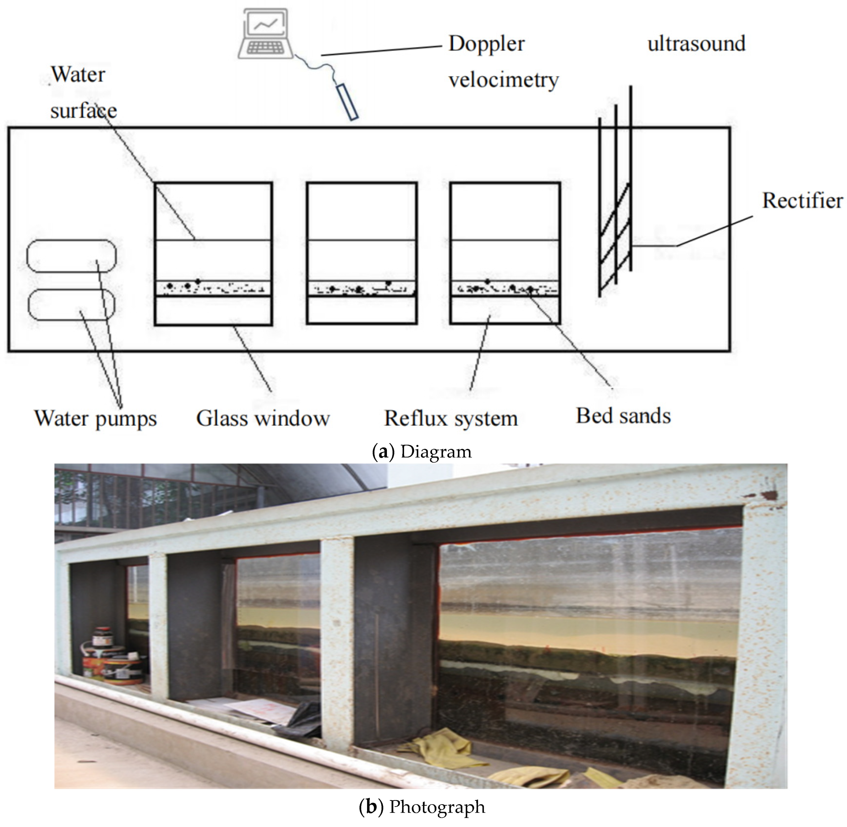
2.2. Experiment Setup
2.3. Test Procedure
2.4. Data Collection
3. Results and Analysis
3.1. Experimental Results and Data Collection
3.1.1. Experimental Results
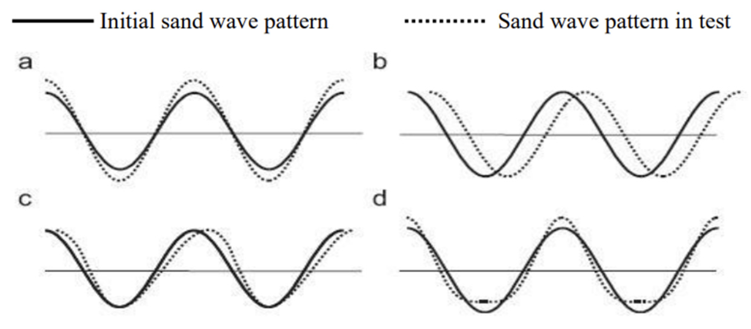
3.1.2. Bedform Development
3.2. Calculation of Bedform Dimensions
3.2.1. Formula Derivation
3.2.2. Parameter Analysis
- (1)
- Momentum Boundary-Layer Thickness
- (2)
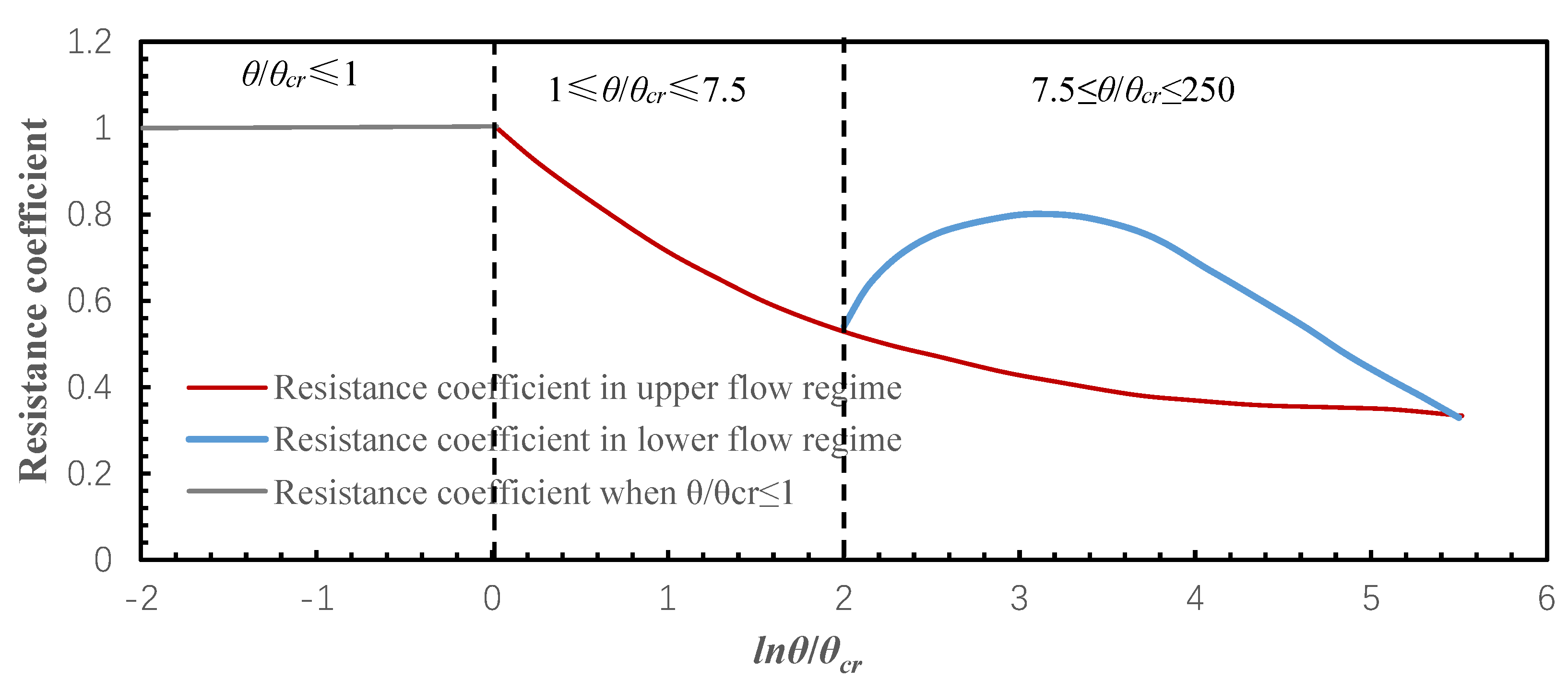
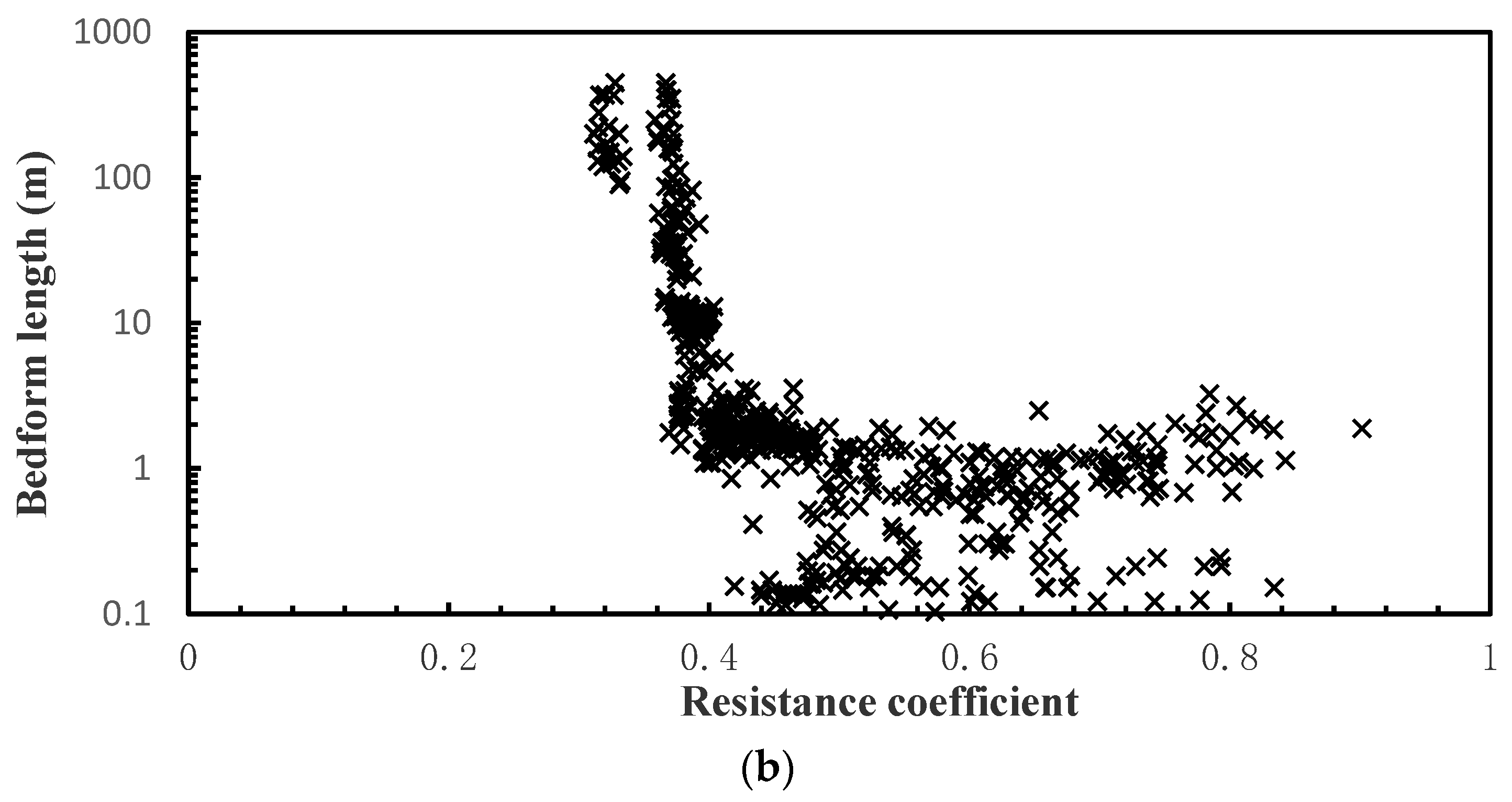
- Resistance Coefficient for Flow in Different Regimes
- (3)
- Flow Intensity
- (4)
- Hydraulic Radius
3.2.3. Coefficient Determination
- (1)
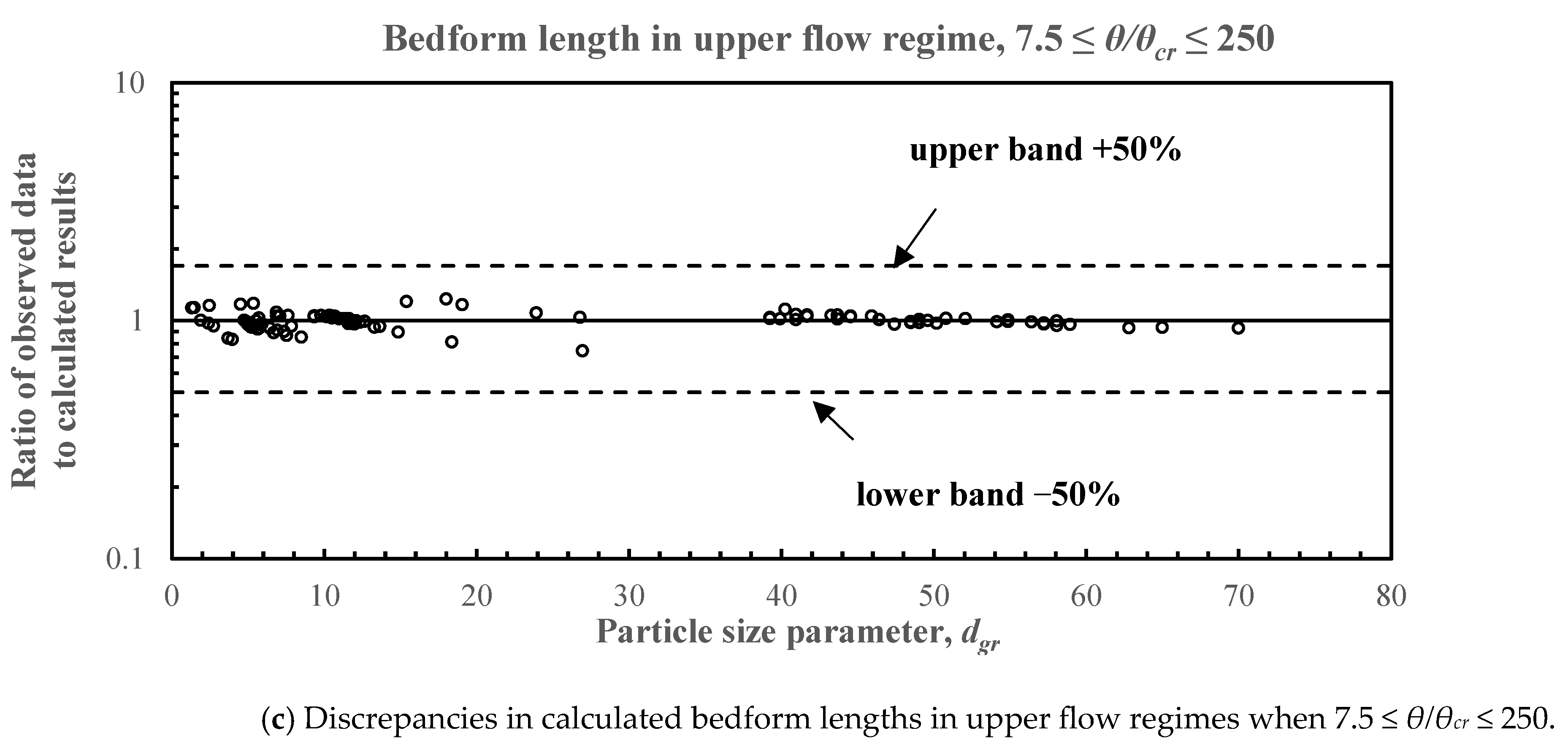
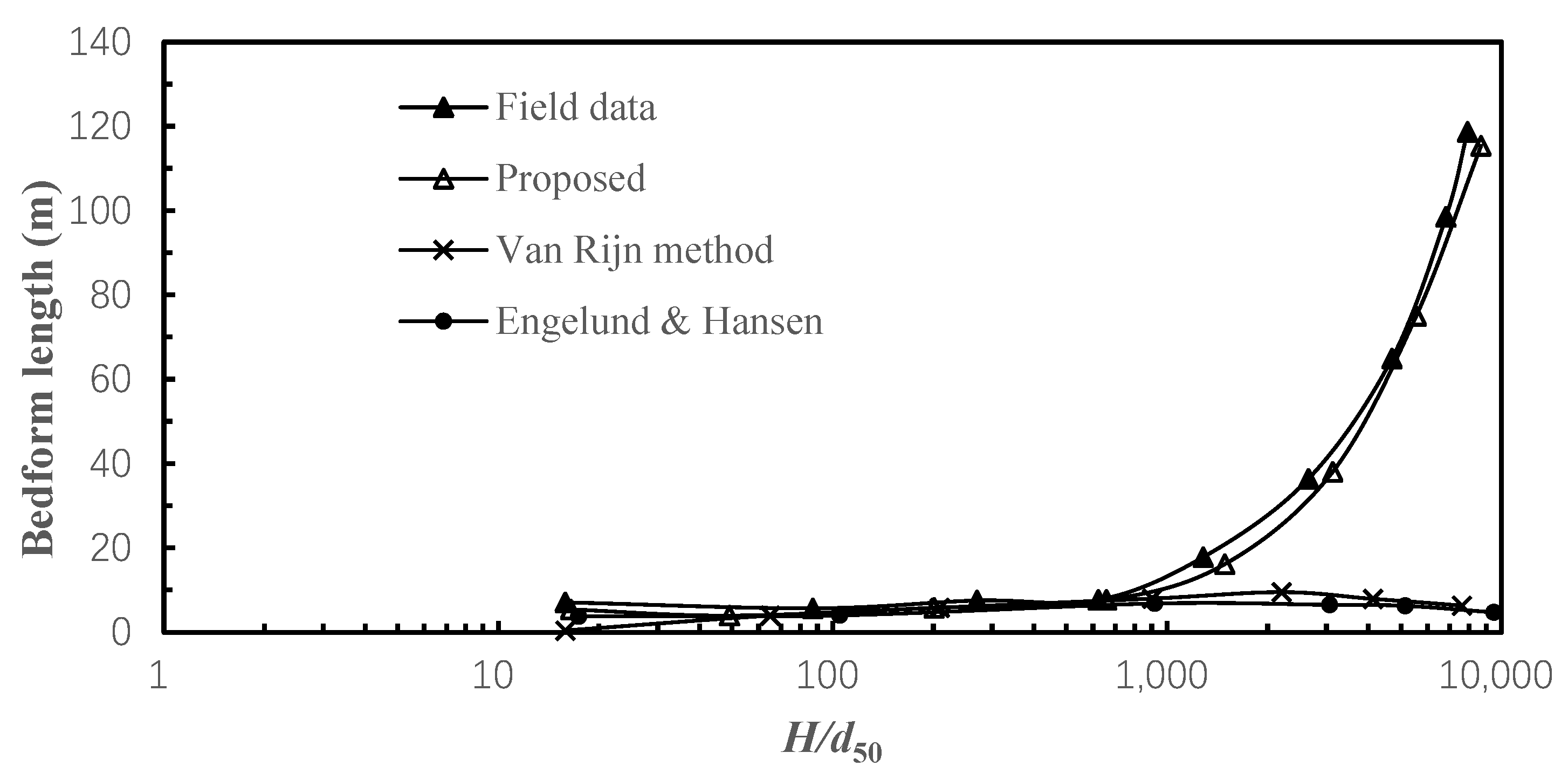
- Bedform Length
- (2)
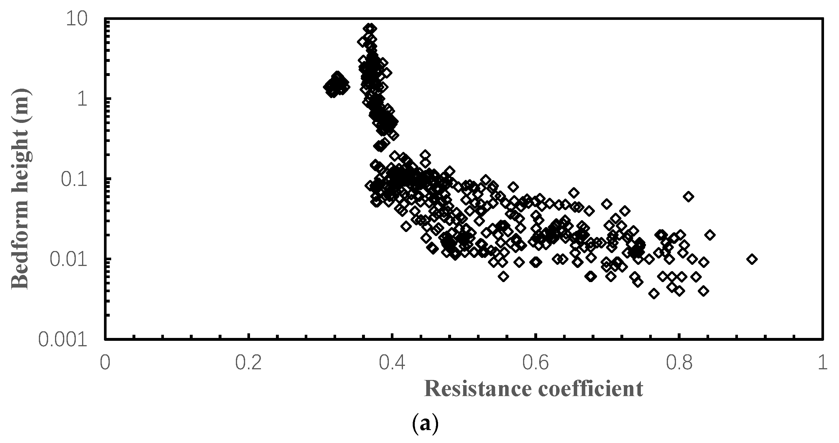
- Bedform Height
- (3)
- Influence of Dimensionless Sediment Particle Size
3.3. Comparison with Other Methods
- (1)
- van Rijn method
- (2)
- Engelund and Hansen Method
- (3)
- Raju and Soni Method
- (4)
- Wuhan Hydropower Institute Method
4. Conclusions
Author Contributions
Funding
Data Availability Statement
Conflicts of Interest
References
- Lefebvre, A.; Herrling, G.; Becker, M.; Zorndt, A.; Krämer, K.; Winter, C. Morphology of estuarine bedforms, Weser Estuary, Germany. Earth Surf. Process. Landf. 2021, 47, 242–256. [Google Scholar] [CrossRef]
- Zhang, P.; Sherman, D.J.; Pelletier, J.D.; Ellis, J.T.; Farrell, E.J.; Li, B. Quantification and classification of grain-flow morphology on natural dunes. Earth Surf. Process. Landf. J. Br. Geomorphol. Res. Group 2022, 47, 1808–1819. [Google Scholar] [CrossRef]
- Best, J. The fluid dynamics of river dunes: A review and some future research directions. J. Geophys. Res. 2005, 110, F04S02. [Google Scholar] [CrossRef]
- Mcninch, J.; Humberston, J. Radar Inlet Observing System (RIOS) at Oregon Inlet, NC: Sediment transport pathways at a wave-dominated tidal inlet. Shore Beach 2019, 87, 24–36. [Google Scholar]
- Baker, M.R.; Williams, K.; Greene, H.; Greufe, C.; Lopes, H.; Aschoff, J.; Towler, R. Use of manned submersible and autonomous stereo-camera array to assess forage fish and associated subtidal habitat. Fish. Res. 2021, 243, 106067. [Google Scholar] [CrossRef]
- Fogg, J.; Hadley, H. Hydraulic Considerations for Pipelines Crossing Stream Channels; Technical Note 423. BLM/ ST/ST-07/007+2880; U.S. Department of the Interior, Bureau of Land Management, National Science and Technology Center: Denver, CO, USA, 2007; p. 20. Available online: http://www.blm.gov/nstc/library/techno2.htm (accessed on 1 January 2007).
- Afzalimehr, H.; Maddahi, M.R.; Sui, J. Bedform characteristics in a gravel-bed river. J. Hydrol. Hydromech. 2017, 65, 366–377. [Google Scholar] [CrossRef]
- Zhang, D.; Narteau, C.; Rozier, O.; du Pont, S.C. Morphology and dynamics of star dunes from numerical modelling. Nat. Geosci. 2012, 5, 463–467. [Google Scholar] [CrossRef]
- Robert, A.; Uhlman, W. An experimental study on the ripple dune transition, Earth Surf. Process. Landf. 2001, 26, 615–629. [Google Scholar] [CrossRef]
- Fang, H.; Cheng, W.; Fazeli, M.; Dey, S. Bedforms and Flow Resistance of Cohesive Beds with and without Biofilm Coating. J. Hydraul. Eng. 2017, 143, 06017010. [Google Scholar] [CrossRef]
- Venditti, J.G.; Church, M.; Bennett, S.J. Morphodynamics of small-scale superimposed sand waves over migrating dune bed forms. Water Resour. Res. 2005, 41, W10423. [Google Scholar] [CrossRef]
- Stark, N.; Hay, A.E.; Trowse, G. Cost-effective geotechnical and sedimentological early site assessment for ocean renewable energies. In Proceedings of the IEEE 2014 Oceans—St. John’s, St. John’s, NL, Canada, 14–19 September 2014; Volume 978, pp. 4799–4918. [Google Scholar] [CrossRef]
- Borkotoky, A. Study on bedforms and lithofacies structures and interpretation of depositional environment of Brahmaputra River near Nemati, Assam, India. Int. J. Eng. Sci. 2015, 4, 14–20. [Google Scholar]
- Hillier, J.; Smith, M.; Clark, C.; Stokes, C.; Spagnolo, M. Subglacial bedforms reveal an exponential size–frequency distribution. Geomorphology 2013, 190, 82–91. [Google Scholar] [CrossRef][Green Version]
- Ashley, G.M. Classification of large-scale subaqueous bedforms: A new look at an old problem. J. Sediment. Petrol. 1990, 60, 160–172. [Google Scholar]
- Bialik, R.J.; Karpinski, M.; Rajwa, A.; Luks, B.; Rowinski, P.M. Bedform characteristics in natural and regulated channels: A comparative field study on the Wilga River, Poland. Acta Geophys. 2014, 62, 1413–1434. [Google Scholar] [CrossRef]
- Aberle, J.; Nikora, V.; Henning, M.; Ettmer, B.; Hentschel, B. Statistical characterization of bed roughness due to bed forms: A field study in the Elbe River at Aken, Germany. Water Resour. Res. 2010, 46, W03521. [Google Scholar] [CrossRef]
- Flemming, B.W. The role of grain size, water depth and flow velocity as scaling factors controlling the size of subaqueous dunes. In Proceedings of the Marine Sand-Wave Dynamics, International Workshop, Villeneuve-d’Ascq, France, 23–24 March 2000. [Google Scholar]
- Yang, Y.; Melville, B.W.; Macky, G.H.; Shamseldin, A.Y. Experimental study on local scour at complex bridge piers under steady currents with bed-form migration. Ocean Eng. 2021, 234, 109329. [Google Scholar] [CrossRef]
- Hiromi, A.; Shun, N.; Misuzu, T.; Naho, M.; Tomomi, F. Alluvial sediments observed around the Tokai Area at the Present and Past Time—Flow velocity, Bedform and Grain size Distribution. Ann. Gifu Shotoku Gakuen Univ. Fac. Educ. 2014, 53, 105–124. [Google Scholar]
- Guala, M.; Singh, A.; Badheartbull, N.; Foufoula-Georgiou, E. Spectral description of migrating bed forms and sediment transport. J. Geophys. Res. Earth Surf. 2014, 119, 123–137. [Google Scholar] [CrossRef]
- Ikramov, N.; Majidov, T. Effect of bedload sediment natural composition on Geometric and dynamic characteristics of channel forms. Irrig. Melioratsiya 2018, 1, 36–39. [Google Scholar] [CrossRef]
- Bian, S.H.; Xia, D.X.; Chen, Y.L.; Zhao, Y.X. The classification characteristics and developing factors of the sand waves at the Mouth of Jiaozhou Bay. J. Ocean Univ. China Nat. Sci. 2006, 36, 327–330. (In Chinese) [Google Scholar]
- Allen, J.R.L. Sand-wave immobility and the internal master bedding of sand-wave deposits. Geol. Mag. 1980, 117, 437–446. [Google Scholar] [CrossRef]
- Miyata, Y.; Tanaka, C. Effect of grain concentration on bedforms under the upper flow regime. J. Geol. Soc. Jpn. 2011, 117, 133–140. [Google Scholar] [CrossRef][Green Version]
- Abdi, V.; Saghebian, S. The potential of FFNN and MLP-FFA approaches in prediction of Manning coefficient in ripple and dune bedforms. Water Sci. Technol. Water Supply 2021, 21, 20211150. [Google Scholar] [CrossRef]
- Van der Mark, C.F.; Blom, A.; Hulscher, S.J.M.H. Quantification of variability in bedform geometry. J. Geophys. Res. Earth Surf. 2008, 113, F03020. [Google Scholar] [CrossRef]
- Kennedy, J.F.; Odgaard, A.J. An Informal Monograph on Riverine Sand Dunes; U.S. Army Engineer Waterways Experiment Station: Vicksburg, MS, USA, 1991. [Google Scholar]
- Fredsoe, J. Shape and dimensions of stationary dunes in rivers. Am. Soc. Civ. Eng. 1982, 108, 932–947. [Google Scholar] [CrossRef]
- Gill, M.A. Height of sand dunes in open channel flows. Am. Soc. Civ. Eng. 1971, 97, 2067–2074. [Google Scholar] [CrossRef]
- Raju, K.G.R.; Soni, J.P. Geometry of ripples and dunes in alluvial channels. J. Hydraul. Res. 1976, 14, 241–249. [Google Scholar] [CrossRef]
- Van Rijn, L.C. Sediment transport, part III: Bedforms and alluvial roughness. J. Hydraul. Eng. 1984, 110, 1734–1754. [Google Scholar] [CrossRef]
- Yalin, M.S. Geometric properties of sand waves. J. Hydraul. Div. 1964, 90, 105–119. [Google Scholar] [CrossRef]
- Julie, P.J.; Klaassen, G.J. Sand-dune geometry of large rivers during floods. J. Hydraul. Eng. 1994, 121, 657–663. [Google Scholar] [CrossRef]
- Raslan, Y. Geometrical Properties of Dunes. Master’s Thesis, Colorado State University, Fort Collins, CO, USA, 1991. [Google Scholar]
- Santoro, V.C.; Amore, E.; Cavallaro, L.; Cozzo, G.; Foti, E. Sand Waves in the Messina Strait, Italy. J. Coast. Res. 2002, 36, 640–653. [Google Scholar] [CrossRef]
- Karim, F. Bed-form geometry in sand-bed flows. J. Hydraul. Eng. 1999, 125, 1253–1261. [Google Scholar] [CrossRef]
- Qaderi, K.; Maddahi, M.R.; Rahimpour, M.; Masoumi, M. Investigating the capability of two hybrid intelligence methods to predict bedform dimensions of alluvial channels. Water Sci. Technol. 2018, 18, 1706–1718. [Google Scholar] [CrossRef]
- Nikora, V.I.; Hicks, D.M. Scaling relationships for sand wave development in unidirectional flow. J. Hydraul. Eng. 1997, 123, 1152–1156. [Google Scholar] [CrossRef]
- Coleman, S.E.; Nikora, V.I. A unifying framework for particle entrainment. Water Resour. Res. 2008, 44, W04415. [Google Scholar] [CrossRef]
- Coleman, S.E.; Zhang, M.H.; Clunie, T.M. Sediment-wave development in subcritical water flow. J. Hydraul. Eng. 2005, 31, 106–111. [Google Scholar] [CrossRef]
- Sami, A.; Hassan, N. Bedform effect on the bed-load transport rate using a comparison between two bedform (flat and standing bedform). Period. Eng. Nat. Sci. 2020, 8, 430–437. [Google Scholar] [CrossRef]
- Wang, R.; Yu, G.L. Incipient condition of sediment motion in great dimensionless flow depth. Appl. Ecol. Environ. Res. 2019, 17, 9837–9863. [Google Scholar] [CrossRef]
- Yu, G.L.; Lim, S.Y. Modified manning formula for flow in alluvial channels with sand-Beds. J. Hydraul. Res. 2003, 41, 597–608. [Google Scholar] [CrossRef]
- Laursen, E.M. Total sediment load of streams. J. Hydraul. Div. 1958, 84, 15301–153036. [Google Scholar] [CrossRef]
- Stein, R.A. Laboratory study of total load and apparent bed load. J. Geol. Res. 1965, 70, 1831–1842. [Google Scholar] [CrossRef]
- Guy, H.P.; Simons, D.B.; Richardson, E.V. Summary of Alluvial Channel Data from Flume Experiments, 1956–1961, USGS Professional Paper, 462-I; U.S. Government Printing Office: Washington, DC, USA, 1966. [Google Scholar]
- Williams, G.P. Flume Experiments on the Transport of Coarse Sand, USGS Professional Paper, 562-B; United States Government Printing Office: Washington, DC, USA, 1967. [Google Scholar]
- Vanoni, V.A.; Brooks, N.H. Laboratory studies of the roughness and suspended load of alluvial streams. Report E-68, Sedimentation Lab. Calif. Inst. Tech. 1957, p. 121. Available online: https://core.ac.uk/download/pdf/216149882.pdf (accessed on 28 February 2024).
- Williams, G.P. Flume width and water depth effects in sediment-transport experiments, USGS Professional Paper, 562-H. 1970. Available online: https://pubs.usgs.gov/pp/0562h/report.pdf (accessed on 28 February 2024).
- Hung, C.S.; Shen, H.W. Statistical analysis of sediment motions on dunes. J. Hydraul. Div. 1979, 105, 213–221. [Google Scholar] [CrossRef]
- Wang, W.C.; Shen, H.W. Statistical properties of alluvial bed forms. In Proceedings of the Third International Symposium on Stochastic Hydraulics, Tokyo, Japan; 1980; pp. 371–389. [Google Scholar]
- Termes, A.P. Watermovement over a Horizontal Bed and Solitary Sanddune. Master’s Thesis, Hydraulic Engineering, University of Delft, Delft, The Netherlands, 1984. [Google Scholar]
- Brown, F. Sediment Transport in River Channels at High Stage. Mphil Thesis, University of Birmingham, Birmingham, UK, 1995. [Google Scholar]
- Ayyoubzadeh, A. Hydraulic Aspects of Straight-Compound Channel Flow and Bed Load Sediment Transport. Ph.D. Dissertation, Department of Civil and Environmental Engineering, University of Birmingham, Birmingham, UK, 1996. [Google Scholar]
- Traykovski, P.; Hay, A.E.; Irish, J.D.; Lynch, J.F. Geometry, migration, and evolution of wave orbital ripples at LEO-15. J. Geophys. Res. Ocean 1999, 104, 1505–1524. [Google Scholar] [CrossRef]
- Marsh, S.W.; Vincent, C.E.; Osborne, P.D. Bedforms in a laboratory wave flume: An evaluation of predictive models for bedform wavelengths. J. Coast. Res. 1999, 15, 624–634. [Google Scholar]


| Sand Samples | Grain Density (g/cm3) | Median Particle size (mm) | Sand Gradation | Sorting Coefficient |
|---|---|---|---|---|
| Natural sand | 2.02 | 0.73 | 1.35 | 2.11 |
| Uniform plastic particles | 1.05 | 3.04 | 1.13 | - |
| Flow Regimes | Upper Flow Regime | Transition Flow Regime | Lower Flow Regime |
|---|---|---|---|
| Bedform | a. Sand grain b. Sand ridge | Flat bed, from ridge to retrograde ridge | a. Flat bed b. Retrograde ridges and standing waves c. Sharp shoals and deep pools |
| Authors | Q (l/s) | B (m) | H (mm) | S0 × 1000 | d50 (mm) | σg | Δ (mm) | λ (m) |
|---|---|---|---|---|---|---|---|---|
| Laursen, 1958 [45] | 24.44~181.9 | 0.914 | 76.2~303.3 | 0.55~2.1 | 0.11 | 1.2 | 19.2~33.5 | 0.116~0.155 |
| Stein, 1965 [46] | 84.38~410.58 | 1.29 | 121.9~346.9 | 2.01~3.87 | 0.399 | 1.5 | 48.8~100.6 | 1.372~3.414 |
| Guy et. al, 1966 [47] | 28.32~603.70 | 0.61~2.44 | 57.9~405.4 | 0.15~10.7 | 1.25~2.07 | 1.3~2.07 | 1.5~198.1 | 0.122~6.43 |
| Williams, 1967 [48] | 5.40~37.38 | 0.305 | 28.7~157.6 | 1.06~22.2 | 1.349 | 1.2 | 12.0~50.12 | 0.18~3.260 |
| Vanoni et. al, 1967 [49] | 3.34~185.47 | 0.267~1.1 | 23.2~370.6 | 0.39~2.90 | 0.14~0.23 | 1.38~1.46 | 11.3~50.6 | 0.104~0.23 |
| Williams, 1970 [50] | 1.42~162.34 | 0.076~1.2 | 27.1~222.5 | 0.6~26.2 | 1.349 | 1.2 | 4.0~86.0 | 0.12~3.350 |
| Hung & Shen, 1979 [51] | 351~714 | 2.440 | 296.0~356.0 | 1.21~3.24 | 1.21 | 0.51 | 53.3~94.9 | 0.273~1.74 |
| Wang & Shen, 1980 [52] | 374.1~720.78 | 2.438 | 291.11~353.9 | 0.5755~3.798 | 1.12 | 1.51 | 19.8~54.3 | 1.152~1.77 |
| Termes, 1984 [53] | 101~441 | 1.00 | 168.0~388.0 | 2.737~3.118 | 0.44~0.51 | 1.7 | 62~151 | 1.557~4.76 |
| Brown, 1995 [54] | 125.5~448.75 | 1.756~1.96 | 56.0~356.6 | 1.633~1.847 | 0.8 | 1.3 | 70.6~118.9 | 1.352~1.95 |
| Ayyoubzadeh, 1996 [55] | 4.86~21.14 | 0.400 | 33.6~113.6 | 1.99~2.19 | 0.8 | 1.3 | 3.7~26.2 | 0.68~1.015 |
| Rivers | Q (l/s) | B (m) | H (m) | S0 × 1000 | d50 (mm) | σg | Δ (mm) | λ (m) |
|---|---|---|---|---|---|---|---|---|
| Missouri | 8.44 × 10⁵~9.83 × 10⁵ | 154.87~201.11 | 3.26~4.47 | 1295~1740 | 0.2 | 1.35 | 77~282 | 4.6~12.98 |
| Zaire | 1.99 × 10⁷~2.85 × 10⁷ | 913.42~1004.28 | 9.5~17 | 5040~6340 | 0.345 | 1.58 | 1200~1900 | 90~450 |
| Waal | 5.25 × 10⁶~6.25 × 10⁶ | 359.64~429.74 | 8~9.5 | 1357~2019 | 0.48~0.85 | 3.3~3.8 | 700~900 | 9~14 |
| Jamuna | 5 × 10⁶~107 | 258.13~813.01 | 8.2~19.5 | 7000 | 0.2 | 1.5 | 800~5100 | 15~251 |
| Parana | 2.5 × 10⁷ | 641.03~1136.36 | 22~26 | 500 | 0.37 | 1.5 | 3000~7500 | 100~450 |
| Bergsche Maas | 2.16 × 10⁶ | 146.05~248.28 | 5.8~10.5 | 1250 | 0.18~0.52 | 1.5 | 400~2500 | 6~50 |
| Meuse | 1.16 × 10⁶~1.74 × 10⁶ | 124.6~210.58 | 6.7~9.52 | 1250~1414 | 0.5~0.65 | 0.58~4.81 | 350~850 | 5.5~13.42 |
| No. | Flow Depth (cm) | Mean Velocity (cm/s) | S0 × 103 | Height (cm) | Length (cm) |
|---|---|---|---|---|---|
| 1 | 15.1 | 43.95 | 1.278 | 3.04 | 32.12 |
| 2 | 16.0 | 42.16 | 1.089 | 3.28 | 33.07 |
| 3 | 17.2 | 41.62 | 0.964 | 3.59 | 34.57 |
| 4 | 17.9 | 41.12 | 0.892 | 4.08 | 32.24 |
| 5 | 19.1 | 39.87 | 0.769 | 4.01 | 33.01 |
| 6 | 20.1 | 38.86 | 0.683 | 4.13 | 32.37 |
| 7 | 21.0 | 37.80 | 0.609 | 3.83 | 29.91 |
| 8 | 21.9 | 37.54 | 0.568 | 3.62 | 27.39 |
| 9 | 23.0 | 36.65 | 0.507 | 2.82 | 26.95 |
| 10 | 24.1 | 37.71 | 0.505 | 2.79 | 24.53 |
| No. | Flow Depth (cm) | Mean Velocity (cm/s) | S0 × 105 | Height (cm) | Length (cm) |
|---|---|---|---|---|---|
| 1 | 28.57 | 8.45 | 3.25 | 2.00 | 69.00 |
| 2 | 28.57 | 9.59 | 4.19 | 2.25 | 82.00 |
| 3 | 28.57 | 10.30 | 4.83 | 2.63 | 90.00 |
| Bedform Type | a0 | a1 | a2 | a3 | a4 | a5 | a6 | R2 | Dataset Number |
|---|---|---|---|---|---|---|---|---|---|
| Lower flow regime | 4.73 | 0.16 | −1.30 | 1.89 | 0.68 | 0.66 | 0.03 | 0.89 | 534 |
| Upper flow regime (θ/θcr ≤ 7.5) | 11.12 | −1.32 | −0.40 | 0.05 | −0.042 | −0.37 | 0.04 | 0.99 | 63 |
| Upper flow regime (7.5 ≤ θ/θcr ≤ 250) | 4.81 | −1.22 | −0.13 | −0.03 | −0.09 | 0.12 | 0.09 | 0.99 | 118 |
| Bedform Type | a0 | a1 | a2 | a3 | a4 | a5 | a6 | R2 | Dataset Number |
|---|---|---|---|---|---|---|---|---|---|
| Lower flow regime | −0.02 | −0.11 | −0.52 | 0.01 | 0.18 | −2.92 | 0.54 | 0.94 | 534 |
| Upper flow regime θ/θcr ≤ 7.5 | 1.23 | 0.09 | 2.92 | −0.43 | −0.04 | 0.06 | 0.95 | 0.96 | 63 |
| Upper flow regime (7.5 ≤ θ/θcr ≤ 250) | −−0.08 | −0.85 | −1.80 | 0.26 | −0.11 | 0.48 | −0.10 | 0.89 | 118 |
| Flow Regime | Lower Flow Regime | Upper Flow Regime | ||||
|---|---|---|---|---|---|---|
| Flow Intensity | - | θ/θcr ≤ 7.5 | 7.5 ≤ θ/θcr ≤ 250 | |||
| Parameter | Δ | λ | Δ | λ | Δ | λ |
| Pearson coefficient | −0.29 | −0.23 | −0.71 | −0.17 | 0.29 | −0.54 |
| Flow Regime | Lower Flow Regime | Upper Flow Regime | ||||
|---|---|---|---|---|---|---|
| Flow Intensity | - | θ/θcr ≤ 7.5 | 7.5 ≤ θ/θcr ≤ 250 | |||
| Parameter | λ | Δ | λ | Δ | λ | Δ |
| a1dgr | 0.67~0.89 | 1.17~1.79 | 0.02~18.4 | 0.82~1.53 | 0.06~1.64 | 0.03~1.86 |
Disclaimer/Publisher’s Note: The statements, opinions and data contained in all publications are solely those of the individual author(s) and contributor(s) and not of MDPI and/or the editor(s). MDPI and/or the editor(s) disclaim responsibility for any injury to people or property resulting from any ideas, methods, instructions or products referred to in the content. |
© 2024 by the authors. Licensee MDPI, Basel, Switzerland. This article is an open access article distributed under the terms and conditions of the Creative Commons Attribution (CC BY) license (https://creativecommons.org/licenses/by/4.0/).
Share and Cite
Wang, R.; Yu, G. Prediction of Bedform Dimensions on Alluvial Bed in Unidirectional Flow. Water 2024, 16, 893. https://doi.org/10.3390/w16060893
Wang R, Yu G. Prediction of Bedform Dimensions on Alluvial Bed in Unidirectional Flow. Water. 2024; 16(6):893. https://doi.org/10.3390/w16060893
Chicago/Turabian StyleWang, Rui, and Guoliang Yu. 2024. "Prediction of Bedform Dimensions on Alluvial Bed in Unidirectional Flow" Water 16, no. 6: 893. https://doi.org/10.3390/w16060893
APA StyleWang, R., & Yu, G. (2024). Prediction of Bedform Dimensions on Alluvial Bed in Unidirectional Flow. Water, 16(6), 893. https://doi.org/10.3390/w16060893