A Data Assimilation Methodology to Analyze the Unsaturated Seepage of an Earth–Rockfill Dam Using Physics-Informed Neural Networks Based on Hybrid Constraints

Abstract

Data assimilation for unconfined seepage analysis has faced significant challenges due to hybrid causes, such as sparse measurements, heterogeneity of porous media, and computationally expensive forward models. To address these bottlenecks, this paper introduces a physics-informed neural network (PINN) model to resolve the data assimilation problem for seepage analysis of unsaturated earth–rockfill dams. This strategy offers a solution that decreases the reliance on numerical models and enables an accurate and efficient prediction of seepage parameters for complex models in the case of sparse observational data. For the first attempt in this study, the observed values are obtained by random sampling of numerical solutions, which are then contributed to the synchronous constraints in the loss function by informing both the seepage control equations and boundary conditions. To minimize the effects of sharp gradient shifts in seepage parameters within the research domain, a residual adaptive refinement (RAR) constraint is introduced to strategically allocate training points around positions with significant residuals in partial differential equations (PDEs), which could facilitate enhancing the prediction accuracy. The model’s effectiveness and precision are evaluated by analyzing the proposed strategy against the numerical solutions. The results indicate that even with limited sparse data, the PINN model has great potential to predict seepage data and identify complex structures and anomalies inside the dam. By incorporating coupling constraints, the validity of our PINN model could lead to theoretically viable applications of hydrogeophysical inversion or multi-parameter seepage inversion. The results show that the proposed framework can predict the seepage parameters for the entire research domain with only a small amount of observation data. Furthermore, with a small amount of observation data, PINNs are able to obtain more accurate results than purely data-driven DNNs.

1. Introduction

Underground seepage analysis has been of great significance in geotechnical engineering, groundwater hydrology, and geophysical hydrology [1,2]. With respect to earth–rock dams, earthen embankments may occasionally experience internal erosion and structural instability due to seepage anomalies within the embankments or foundations. Because underground seepage is usually found in areas that are relatively difficult to directly observe, relying solely on experimental methods may not be sufficient to gain a comprehensive understanding of this complex phenomenon, let alone accurately predict trends. As a complementary alternative to experimental research, numerical simulation can play a vital role in improving scientific prediction capabilities by constructing mathematical models that accurately describe complex physical behaviors. In this sense, accurate modeling of seepage analysis requires precise quantitative information, which involves the distribution of medium parameters. For instance, parameters like permeability and porosity directly affect the redistribution of seepage within an earth–rockfill dam [3] in the seepage model. Similarly, parameters including concentration, location, and permeability of porous media play a critical role in accurately predicting the distribution of downstream pollutant concentrations in models of underground pollutant migration [4]. In addition, the precise characterization of reservoir rock properties, such as permeability, porosity, and other relevant parameters, is crucial for oil production prediction [5]. In fact, significant spatial heterogeneity is typically observed in parameters linked to porous media. Factors such as the number and distribution range of wells can affect the accuracy of the distribution of subsurface hydrological parameters during intrusive hydrogeological testing. Furthermore, these parameters often exhibit a scaling effect, which can lead to uncertainties when extrapolating small-scale models to larger study areas using various scaling strategies. This essentially restricts the advancement of seepage analysis and makes it difficult to fully understand underground seepage through numerical simulation.

Within this context, data assimilation has drawn a significant amount of attention in the underground seepage field, especially for parameters inversion. It also holds great importance to use indirect observation data, which are relatively easier to obtain but sparse, to infer the seepage parameters in the case of complex seepage problems. Since the ensemble Kalman filter (EnKF) was proposed by Evensen [6], a data assimilation approach that uses a set of samples has been successfully utilized in various fields, such as meteorology [7], hydrology [8], petroleum [9], remote sensing [10], etc. Derivative algorithms have been developed to address specific issues in these domains. In addition to EnKF and its derivatives, several other probability estimation methods have also been proposed for the data assimilation of subsurface seepage, including generalized likelihood uncertainty estimation [11], Markov chain Monte Carlo [12], hydraulic tomography [13], and the particle-filter instrument method [14].

Previous studies have established that a specific numerical model can accurately represent the underlying physical process [15,16]. However, numerical models may not fully comprehend all the processes of reality when addressing complex issues. In fact, improper numerical models during the data assimilation process can impact parameter estimation and compromise the reliability of future predictions. The potential of recent deep learning frameworks has been demonstrated for applications like automatic analysis [17], rule extraction [18], and prediction of unknown states based on sparse data [19]. The process of acquiring knowledge from limited, sparse data has been greatly facilitated by the increase in computational power and continual improvement in deep learning models. Mao et al. [20] utilized deep learning techniques to obtain prior velocity information using 5000 forward models that acted as a driving force for data assimilation. Tang et al. [21] combined convolutional neural networks with recurrent neural networks (RNNs) for data assimilation in channelized systems, which dramatically reduced prediction uncertainty. The reported method has also been extended to the three-dimensional case [22]. Kang et al. [23] proposed the integration of the convolutional autoencoder (CAVE) with the Kalman filter for assimilating time-delay hydrogeophysical observation data. Their approach’s effectiveness was attributed to a dataset that included 30,000 training samples and 3000 test samples. The enlightenment of these implementations shows that traditional data-driven deep learning methods often prioritize data learning while ignoring the effective integration of fundamental physical laws and physics-informed constraints. Improving the network’s generalizability requires using more training datasets and extending the training duration. However, the process of acquiring hydrological parameters, crucial for data-driven deep learning, could be rather difficult and may result in sparse or noisy labeled data. Furthermore, the cost associated with obtaining label data, even through numerical simulation methods or experiments, is quite high [24], making it extremely difficult to construct large training datasets.

Instead of learning solely from hydrological data (e.g., solution of the states on certain points in parameter space), the already known governing equations can also be utilized to constrain (or even drive) the learning process to compensate for the data insufficiency. Some studies have explored the integration of both approaches to exploit their respective strengths and overcome this limitation. Raissi et al. [25] proposed a neural network to solve non-linear partial differential equations (PDEs) for forward and inverse problems, which represents the prototype of physics-informed neural networks (PINNs). The successful application of PINNs for parameter estimation has achieved milestones since then. To determine nano-optical materials’ permittivity parameters, Chen et al. [26] employed PINNs and compared them to numerical solutions obtained by the finite element method. For dynamic prediction for the petroleum industry, Xue et al. [27] developed a deep network model for pressure field determination driven by reservoir physics-data seepage, with a performance comparable to a purely data-driven neural network.

In the underground seepage field, PINNs have also been employed to predict the saturated seepage parameters. Tartakovsky et al. [28] employed PINNs to estimate the heterogeneous permeability and the permeability function that alters as the hydraulic head increases. He et al. [29] presented a multi-physics-informed deep neural network for estimating space-dependent hydraulic conductivity, hydraulic head, and concentration fields. Zhang et al. [30] incorporated soft and hard constraints into PINNs for both forward and inverse calculations in groundwater seepage models. In contrast, only a few studies have been conducted on the problem of unsaturated seepage using PINN techniques. Depina et al. [31] utilized PINNs to calculate unsaturated groundwater flow by making use of Richards’ equation to obtain the parameters of the van Genuchten model. Shadab et al. [32] predicted phreatic surface profiles using PINNs.

However, predicting parameters for saturated–unsaturated seepage analysis is still a challenge, particularly in the case of earth–rockfill dams with limited sparse data. The difficulties remain unsolvable because the unsaturated and saturated–unsaturated areas of earth–rockfill dams have distinct characteristics (such as hydraulic conductivity) that differ from the saturated areas. In reality, the gradients of seepage parameters exhibit a dramatic change not only at the interface between saturated and unsaturated areas but also at the boundaries of abnormal bodies [33]. The initial PINNs framework has encountered issues with accurately estimating seepage parameters [25] since the training points are chosen randomly, through which the process may inevitably miss those domains where the seepage parameters are distributed with dramatic variations.

To mitigate this impact, the residual adaptive refinement (RAR) [34] is introduced for the first attempt to strategically add training points around locations with high residuals of the PDEs, which could thereby guarantee the enhancement in prediction accuracy. Building upon previous research [35], this study also utilizes the smoothed finite element method (SFEM) for forward computation to first verify and obtain the numerical solutions (i.e., water head (h), hydraulic conductivity (k)). More importantly, the numerical solutions are subsequently randomly sampled to generate observed values, which are then employed with the seepage control equation, and boundary conditions are informed as the hybrid constraints in the loss function. To optimize, we combine both the Adam and the L-BFGS algorithms to train neural networks simultaneously, upon which the number of training epochs can be adjusted automatically when faced with different problems. Through extensive comparisons and analysis, we reported the prediction accuracy of the proposed methodology against numerical solutions and demonstrated its stability in addressing prediction challenges in complex earth–rockfill dam applications.

2. Methods

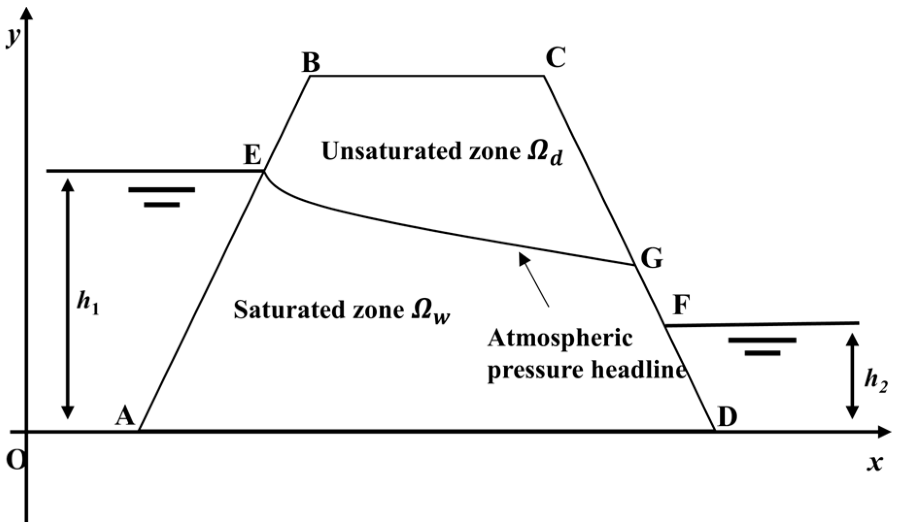
2.1. Seepage-Governing Equation

The problem of unsaturated pressure-free seepage of the earth–rockfill dams is illustrated in Figure 1. The research domain is divided into saturated zone Ω_w and unsaturated zone Ω_d by the atmospheric pressure headline EG.

The PDEs of governing flow derived by Richards [36] assume that the flow follows Darcy’s law independent of soil saturation. Under steady flow conditions, the net flow of a soil unit shall be zero. In cases where the maximum or minimum hydraulic conductivity is parallel to the x-axis or y-axis, the PDE governing the flow can be expressed as follows:

$$\frac{\partial }{\partial x}(k_x(u_w)\frac{\partial h}{\partial x})+\frac{\partial }{\partial y}(k_y(u_w)\frac{\partial h}{\partial y})=0,$$

(1)

where h is the total head (i.e., pressure head plus elevation head); k_x(u_w) and k_y(u_w) are the hydraulic conductivities in the x and y directions, respectively, which are dependent upon the pore water pressure u_w.

The boundary conditions of the equation describe the hydraulic properties at the geometric boundary of the seepage region. As illustrated in Figure 1, the corresponding boundary conditions are as follows:

(1) The boundary conditions of AE and DF head of upstream and downstream reservoir water are

$$h(x,y){\mid }_{{\Gamma }_1}=h_0(x,y).$$

(2)

(2) The bottom boundary (AD) is impermeable and meets the discharge boundary condition:

$$q_n{\mid }_{{\Gamma }_2}=v\cdot n=0,$$

(3)

where v is the velocity, n is the vector of the upward normal unit, and the flow rate in the upward normal direction is equal to zero.

The saturated–unsaturated seepage theory posits that the hydraulic conductivity of soil depends not only on the soil properties but also on the soil matrix suction. Since the pore air pressure equals atmospheric pressure, matrix suction is also equal to the negative pore water pressure. The volumetric water content function describes the stored water volume as a function of matric suction (φ), which is equivalent to negative pore water pressure when the air pressure is zero. Hydraulic conductivity is a function of volumetric water content and, thus, indirectly, a function of pore water pressure.

Van Genuchten [37] proposed a simple soil water content pressure head curve equation and derived a closed analytical expression for the hydraulic conductivity coefficient in the unsaturated zone through a special form of the equation. According to a technique developed by van Genuchten, the unsaturated zone volumetric water content function can be generated using a closed-form equation requiring curve-fitting parameters:

$${\theta }_w={\theta }_{res}+\frac{{\theta }_{sat}-{\theta }_{res}}{{\left[1+{\left(\alpha \phi \right)}^n\right]}^m}$$

(4)

The hydraulic conductivity function is estimated from the saturated hydraulic conductivity and volumetric water content functions. The parameters in the equation are generated from the curve-fitting parameters of the volumetric water content function and the saturated hydraulic conductivity coefficient. The closed-form equation for the hydraulic conductivity coefficient in the unsaturated zone is

$$k_w(\phi )=k_{sat}\frac{{\left\{1-{\left(\alpha \phi \right)}^{n-1}{\left[1+{\left(\alpha \phi \right)}^n\right]}^{-m}\right\}}^2}{{\left[1+{\left(\alpha \phi \right)}^n\right]}^{m/2}}$$

(5)

Among them, α = 0.005, n = 2, and m = 1 − 1/n are the curve-fitting parameters that control the shape of the volumetric water content function. θ_sat is the saturated volumetric water content, which is given as 0.5; θ_res is the residual volume water content, which is given as 0.1; k_sat is the saturated hydraulic conductivity coefficient; and k_w(φ) is the hydraulic conductivity coefficient in the unsaturated zone.

Without loss of generality, this study first employs the smoothed finite element method (SFEM) [35] to perform forward seepage modeling, generate observation data, and validate the effectiveness and precision of the trained surrogate models.

2.2. Neural Network Implementation

2.2.1. Structure of Neural Network

In this paper, a fully connected neural network (FC-NN) architecture was employed, characterized by full interconnection between neurons in adjacent layers. Compared to convolutional neural networks (CNNs) and recurrent neural networks (RNNs), FC-NNs have a simpler and more interpretable structure. It can flexibly learn complex relationships between inputs without assuming specific input order or spatial structure, making it more useful for solving seepage problems that involve different types of input data. The FC-NN structure facilitated the flow of information across the networks, as the output of each layer served as input for the subsequent layer. The specific architecture of the neural network is as follows:

$$N^0(x)=x,x\in R^{d_{in}},$$

(6)

$$N^l(x)=\sigma (W^l{N}^{l-1}(x)+b^l)\in R^{N_l},for 1\le l\le L-1,$$

(7)

$$N^L(\mathit{x})=({\mathit{W}}^L{N}^{L-1}(\mathit{x})+{\mathbf{b}}^L)\in R^{d_{out}}.$$

(8)

where $N^L(\mathit{x}):R^{d_{in}}\to R^{d_{out}}$ represents the architecture of the neural network, indicating that the network consists of a total of L layers, including the input layer and the output layer; N^l(x) represents the neurons in the l-th layer; N⁰ represents the input layer; N^L represents the output layer; σ represents the activation function; and W and b represent the weight matrix and bias vector, respectively.

Figure 2 illustrates the schematic diagram of the seepage data assimilation method based on PINNs. The left portion of the figure depicts the architecture of the FC-NN. This FC-NN architecture comprises four hidden layers, with each hidden layer consisting of 50 neurons. The parameter θ represents the set of parameters in the neural network, including the weights (W) and bias (b). Considering the requirement for computing second-order derivatives in solving the PDE of the seepage field, the tanh function, which is infinitely differentiable, is employed as the activation function. To initialize the parameters of the neural network, we employed the Glorot uniform [38], commonly referred to as the Xavier uniform distribution initializer. This method can effectively resolve the tough issues of gradient explosion and gradient vanishing when used in conjunction with the tanh function. The neural network takes the coordinate parameters x and y as inputs, while $\tilde{h}$ and $\tilde{k}$ are the outputs at the current epoch. The middle part of Figure 2 illustrates the components of the loss function, which include the PDE constraint, boundary condition constraint, and observation value constraint. F_N represents the PDE (Equation (1)); B_d represents the Dirichlet boundary condition (Equation (2)); B_n represents the Neumann boundary condition (Equation (3)); n represents the unit orthogonal vector; N is the index of the point used for training; and P represents the index of the observed point and corresponds to its coordinates. The gradient of the network output with respect to the input is calculated by loss function with automatic differentiation (AD) [39], which facilitates subsequent parameter updates using the Adam and L-BFGS optimization algorithms. Through iterative training, optimal neural network parameters θ* are obtained, capable of guaranteeing precise predictions of h and k.

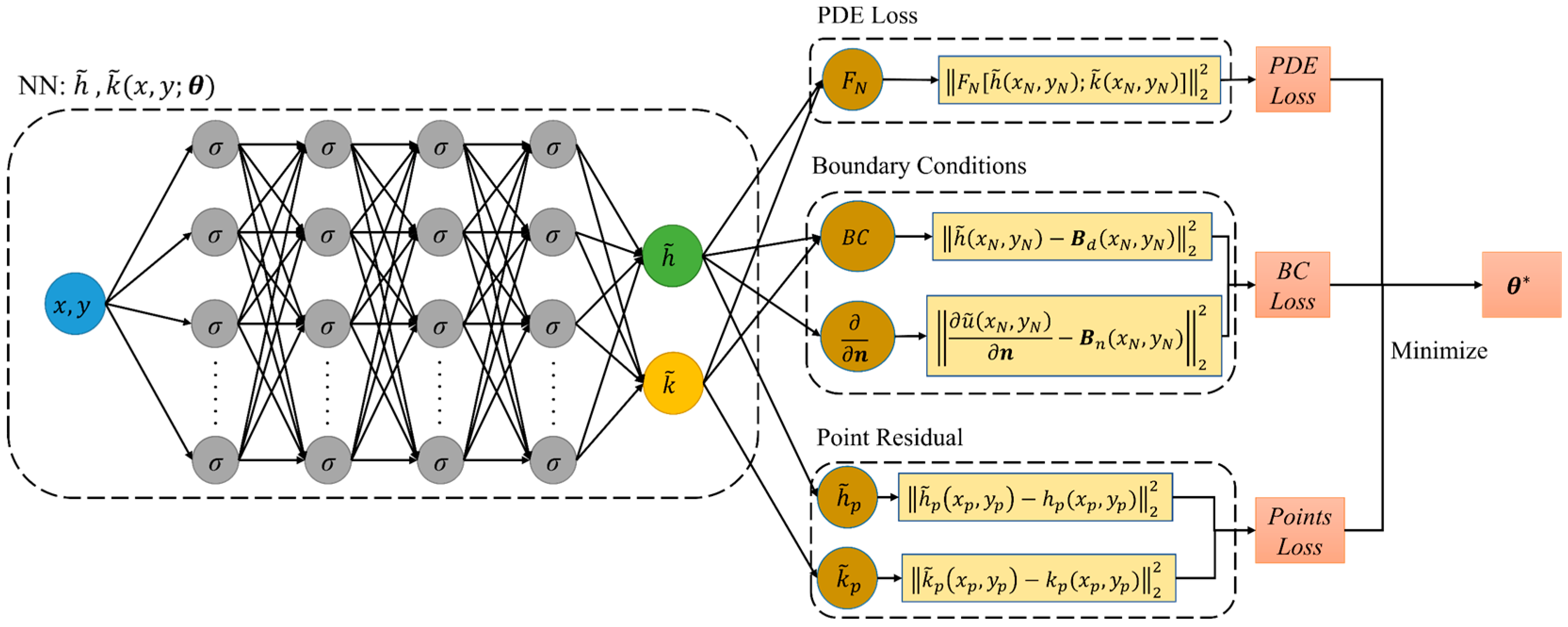
2.2.2. Loss Function

Neural network training is a fundamental process aimed at minimizing the loss function progressively. Since PINNs incorporate PDEs, boundary conditions, and observation data into the loss function, ensuring that the model’s predictions comply with the underlying physical laws. The form of the loss function used in this paper is defined as follows:

$$L(\theta ;\Gamma )=L_f(\theta ;{\Gamma }_f)+L_b(\theta ;{\Gamma }_b)+L_p(\theta ;{\Gamma }_p),$$

(9)

with

$$L_f(\theta ;{\Gamma }_f)=\frac{1}{\left|{\Gamma }_f\right|}{\displaystyle \sum _{x\in {\Gamma }_f}{‖{\nabla }^T(k\nabla h(x))‖}_2^2},$$

(10)

$$L_b(\theta ;{\Gamma }_b)=\frac{1}{\left|{\Gamma }_b\right|}{\displaystyle \sum _{x\in {\Gamma }_b}{‖\mathrm{B}(\tilde{u},x)‖}_2^2},$$

(11)

$$L_p(\theta ;{\Gamma }_p)=\frac{1}{\left|{\Gamma }_p\right|}{\displaystyle \sum _{x\in {\Gamma }_p}{‖\tilde{u}-u‖}_2^2},$$

(12)

where Γ_f and Γ_b are the sets of residual points corresponding to the PDEs and the boundary conditions used for training, respectively. Typically, these residual points are obtained through random sampling within the domain. Additionally, Γ_p represents the set of observation points used to train the neural network; $\tilde{u}$ represents the output (i.e., $\tilde{h}$ and $\tilde{k}$) of the neural network; u represents the corresponding observed values (i.e., h and k); and B represents the boundary conditions associated with the PDEs.

2.2.3. Automatic Differentiation

When applying the PINNs to assimilate seepage data in earth–rockfill dams, it is essential to calculate the derivative of the network output with respect to the input. To accomplish this, we use an automatic differentiation (AD) technique [39], which is an accurate and efficient approach for computing derivatives in a computational graph involving forward propagation and backpropagation. AD calculates the derivative by performing backpropagation on the calculation graph, decomposes the differential process of the function into a series of simple basic operations, and then uses the chain rule to calculate the derivative. Therefore, AD offers more precise derivatives compared to numerical differentiation methods, as it is not affected by truncation or round-off errors. Widely used deep learning frameworks such as TensorFlow [40] and PyTorch [41] incorporate built-in AD modules.

2.2.4. Residual-Based Adaptive Refinement

Since the points used to compute residuals are randomly sampled within the study domain during the training process, it is not guaranteed that the training points have a continuous distribution at steep gradients for the seepage-governing equation whose solution is unknown. Designing an optimal distribution of training points for solving unknown problems remains a difficult task when training neural networks. The model in this study presents intricate internal structures, leading to rapid changes in boundary gradients, which may potentially have an impact on the accuracy of network predictions.

To address this, the RAR algorithm [34] is introduced, which focuses on increasing the density of training points in areas with high residual of the PDE until the mean residual is down to threshold $\epsilon$. This refinement of training points allows the model to capture the behavior of the solution more effectively in gradient distortion regions, thereby enhancing the accuracy of network predictions. This method is used in Section 3.3 for improving the prediction accuracy of the complex model. See

Table 1. The workflow of the RAR method.

Workflow of the RAR Method
Step 1: Select a set of the initial points Γ and train the PINNs for a limited number of iterations.
Step 2: Calculate the mean PDE residual by the average of values at a set of randomly sampled points in area S. Step 3: Stop if the residual is within the threshold. Otherwise, add new points with the largest residual points in S to Γ, retrain the network, and go to Step 2.

for the workflow.

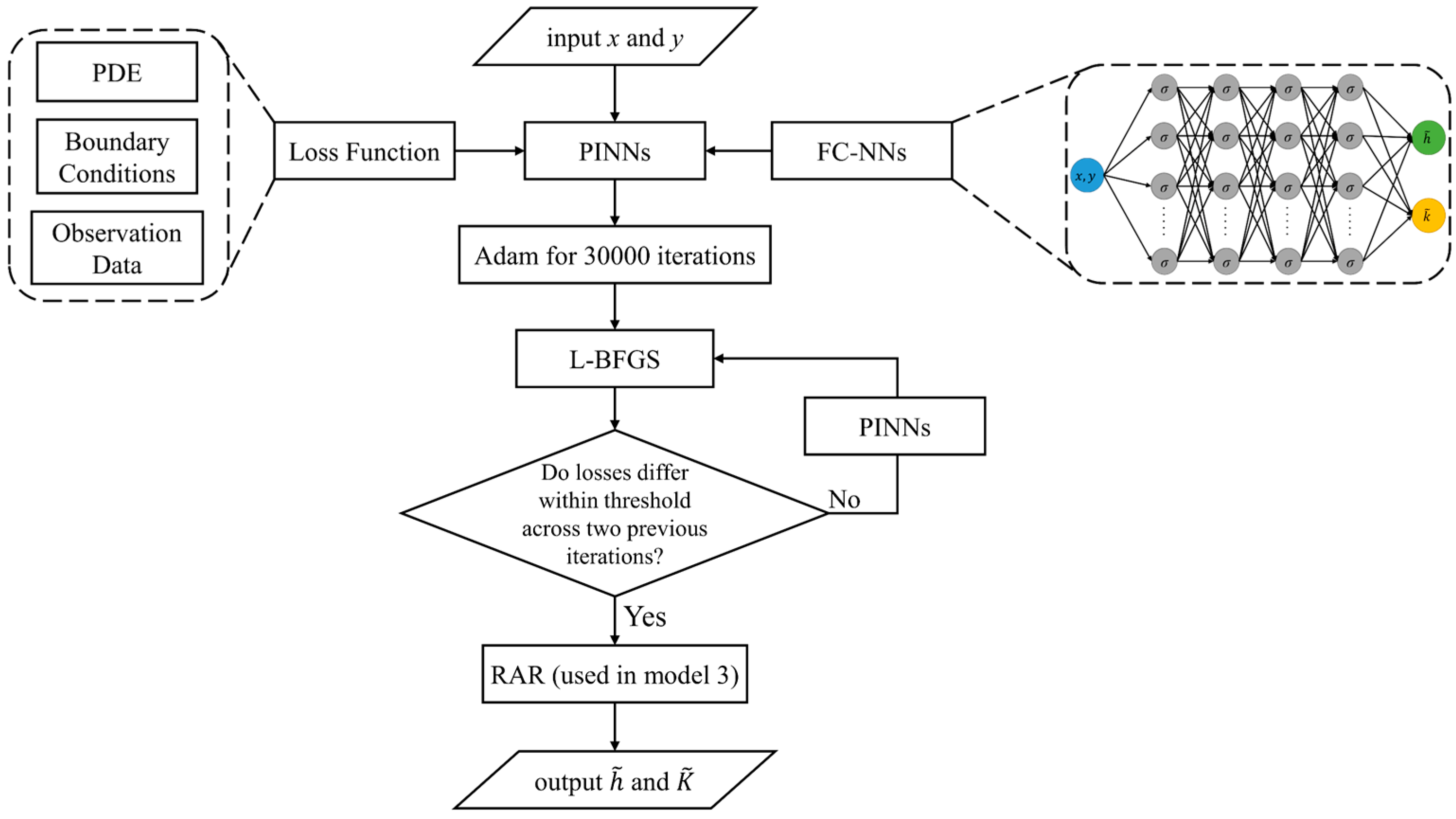
2.2.5. Workflow Process

Here, we give a brief overview of the model training process workflow, which is as follows:

(i)

Construct a PINN with the defined loss function (Equation (9)) and FC-NN. The inputs of the neural network are x and y, and the outputs are h and k.

(ii)

Initialize the network parameters (W and b) using the Glorot uniform.

(iii)

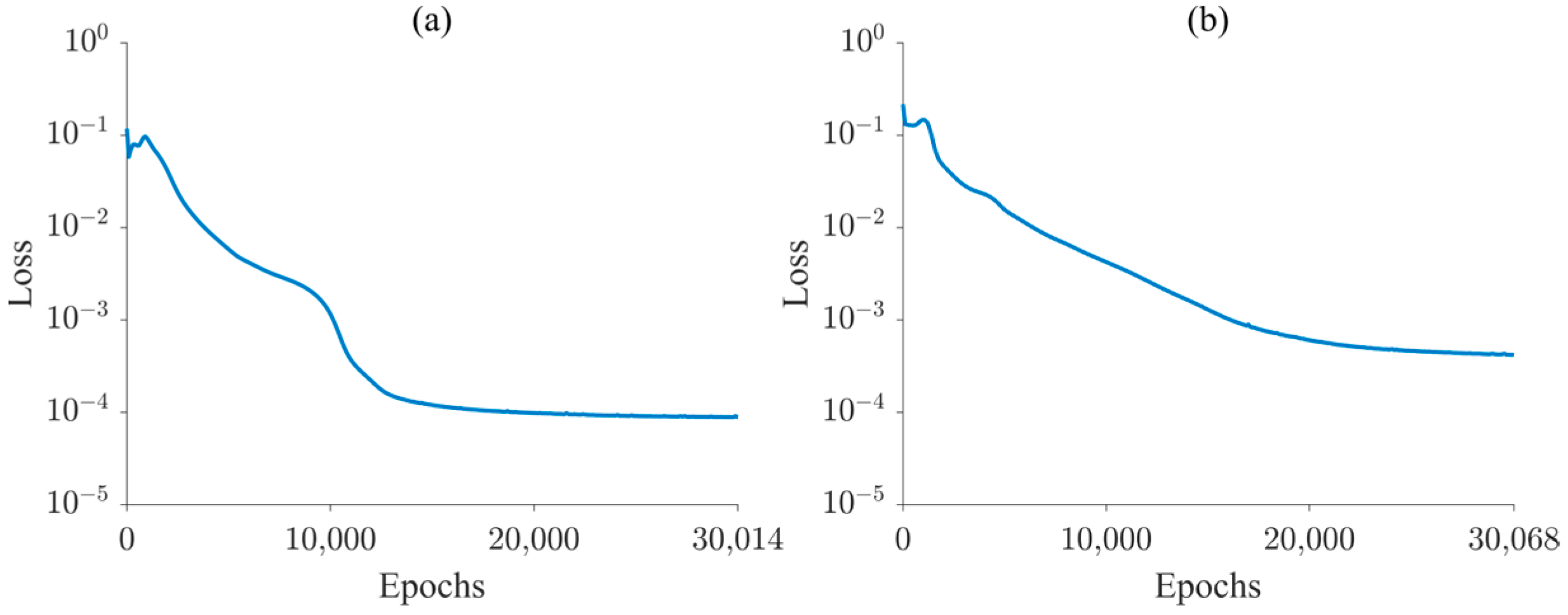
Perform training using the Adam optimization algorithm for 30,000 epochs with a 0.0001 learning rate. Subsequently, switch to the L-BFGS optimization algorithm to continue training until the difference between the loss function values of two consecutive epochs falls below a specified tolerance.

(iv)

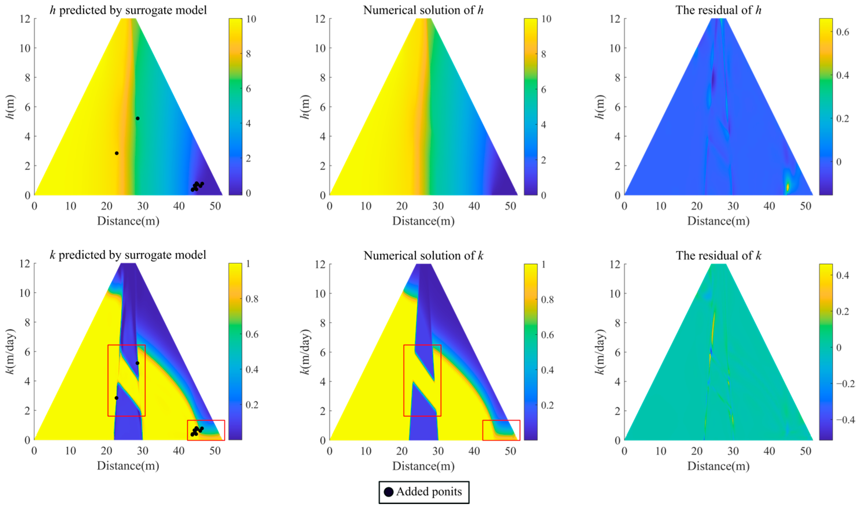
For the complex model in Section 3.3, apply the RAR method to further improve the accuracy of the calculations.

In this paper, L₂ relative errors are used to quantify the error between the prediction results ($\tilde{h}$ and $\tilde{k}$) and the numerical solutions (h and k) and to evaluate the performance of the neural network model:

$${\epsilon }_h=\frac{\sqrt{{\displaystyle {\int }_{\mathrm{\Omega }}{[h(\mathrm{x})-\tilde{h}(\mathrm{x})]}^{2}d\mathrm{x}}}}{\sqrt{{\displaystyle {\int }_{\mathrm{\Omega }}{h}^2(\mathrm{x})d\mathrm{x}}}},$$

(13)

$${\epsilon }_k=\frac{\sqrt{{\displaystyle {\int }_{\mathrm{\Omega }}{[k(\mathit{x})-\tilde{k}(\mathit{x})]}^{2}d\mathit{x}}}}{\sqrt{{\displaystyle {\int }_{\mathrm{\Omega }}{k}^2(\mathit{x})d\mathit{x}}}}$$

(14)

The surrogate model obtained after training can directly predict the seepage field parameters. The training process is illustrated in Figure 3. It should be noted that within the framework of PINNs, both observations of h and k are utilized during the training, allowing simultaneous predictions of h and k. Accordingly, for Equation (1), we can unify the forward problem (solving for state h) and the inverse problem (estimating parameter k) within the PINNs framework and thus achieve the objective of data assimilation.

3. Numerical Experiments

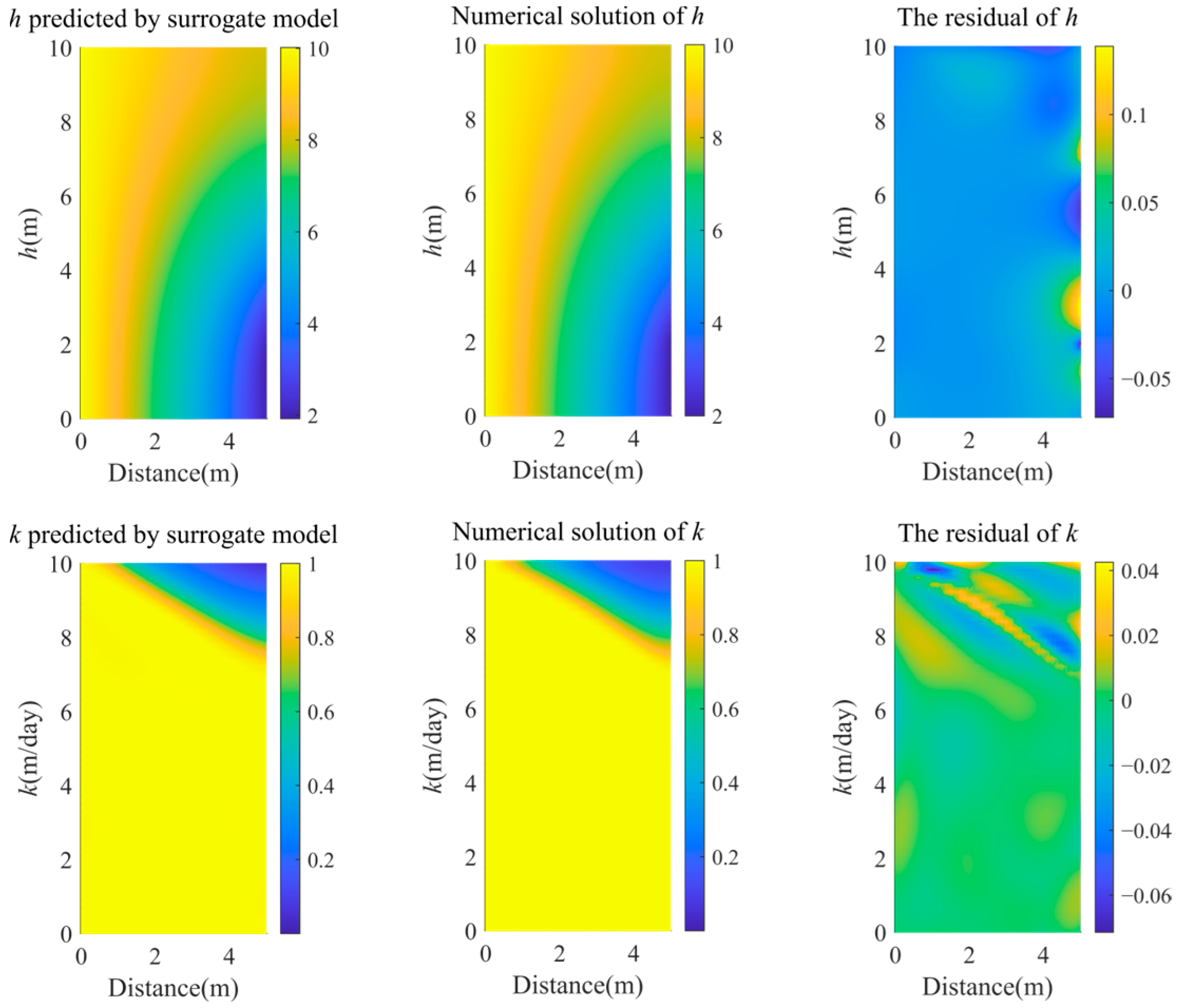
3.1. Homogeneous Rectangular Dam

Model 1 is a typical Muskat problem, in which the dam is 10 m high and 5 m wide, and the water level upstream and downstream are fixed at 10 m and 2 m, respectively. The saturated hydraulic conductivity is set as k_sat = 1 m/day. In the research domain, there are a total of 2091 points; for the numerical solution by SFEM, we randomly sample 60 points as the observed data. During the neural network training, we randomly sample 1024 points within the research domain and 200 points on the boundaries as training points. Figure 4 presents the predicted results of the surrogate model and the comparison with the numerical solution.

The residual analysis demonstrates high consistency between the predicted results of the surrogate model and the numerical solution. This can be attributed to the powerful inference capabilities of deep learning, which allows precise predictions of seepage parameters at arbitrary locations within the research domain once the model training is completed. The L₂ relative errors between the predicted h and k and the numerical solution are as low as 0.0023 and 0.0105, respectively. In addition, the influence of the number of observation points was investigated and shown in Figure 5. This figure also shows the comparison of results between purely data-driven DNNs and the PINN method. For a small number of observation data (in this case, Γ_p < 60), the error in estimated k and h with data-driven DNNs is larger than the error computed with the PINN method. However, when a larger amount of observation data is used for training (Γ_p > 70), the data-driven DNN method starts to be more accurate than the PINN method. Therefore, using sufficient observation data during training can obtain accurate results without physical constraints. Additionally, increasing the number of observation points may further decrease the error. However, in practical engineering, only sparse observation data can often be collected. It can also be seen from this figure that once a sufficient number of observation points is reached, the reduction in prediction error almost disappears, leading only to increasing computational complexity. The convergence curve of the loss function is shown in Figure 6.

The spatial distribution of high errors is graphically represented on the right side of the Figure 4. As well, Figure 7 shows the density distribution of the residual between the predicted results and the numerical solution. The majority of errors for the h and k predictions are concentrated in the range of −0.01–0.01, indicating a close resemblance between the surrogate model predictions and the numerical solution. The integration of hybrid physical constraints into the trained surrogate model is further confirmed by the analysis of the residual diagram presented in Figure 4. This demonstrates that promising prediction results can be achieved under the hybrid constraints of sparse observation points and numerical models.

When exclusively employing the Adam optimization algorithm, multiple experiments are required to determine the optimum number of training epochs. In other words, insufficient training epochs may result in a surrogate model that does not meet the required standards of accuracy. Conversely, excessively high training epochs do not necessarily lead to significant improvements in accuracy since the Adam optimization algorithm works as a stochastic gradient descent algorithm [33]. To address this issue, the L-BFGS optimization algorithm is employed after training with the Adam algorithm to further enhance the accuracy of the network model.

Table 2. The L₂ relative error between the prediction results of the rectangle dam and the numerical solution (each method is calculated independently five times).

	L2 Relative Error of h	L2 Relative Error of k
Adam	0.0028	0.0391
Adam, L-BFGS	0.0029	0.0189

presents the L₂ relative errors for two distinct training strategies. As a result of the training strategy with both Adam and L-BFGS, the need to manually adjust the number of training epochs across different models is eliminated. The number of training epochs automatically adapts to more complex models.

3.2. Trapezoidal Dam

In this section, a homogeneous trapezoidal dam model was designed with 12 m height, 4 m width at the dam top, 52 m width at the dam bottom, and the slope ratio is 1:2. The water levels upstream and downstream are 10 m and 2 m, respectively. The saturated hydraulic conductivity is set as k_sat = 1 m/day. In the research domain, there are a total of 6171 points. For the numerical solution of SFEM, we randomly sample 180 points as the observed data. During the neural network training, we randomly sample 2048 points within the research domain and 400 points on the boundaries as the training points.

Figure 8 shows the surrogate model predictions as compared to the numerical solution. The L₂ relative errors between the predicted h and k and the numerical solution are as low as 0.0045 and 0.0133, respectively. These results demonstrate that the data assimilation method based on PINNs can also provide sufficient stability for irregular geometric models.

In order to verify the prediction performance of PINNs in large-scale point situations. A core wall was designed in the trapezoidal dam model, and the number of points in the study domain was increased to 35,496. We randomly sample 1064 points as the observed data. During the neural network training, we randomly sample 2048 points within the research domain and 400 points on the boundaries as the training points. The results are shown in Figure 9. The L₂ relative errors between the predicted h and k and the numerical solution are as low as 0.0058 and 0.0388, respectively. The errors of these two models were successfully controlled within −0.03–0.03 (Figure 10). Figure 11 presents the convergence curves of the loss function during the training process.

Unlike traditional numerical simulation methods that require fine mesh division for irregular geometries, PINNs possess meshless properties and can be applied to models with arbitrary complex geometries, thus avoiding the need for expensive memory and calculation costs. The proposed methodology does not specify a fixed number of epochs for neural network training. Instead, the training terminates when the loss function reaches a predefined threshold, determined by the specified tolerance (i.e., the difference between the loss function values of two consecutive epochs). Consequently, the number of epochs may differ from one model to another with different structures. As illustrated in Figure 11, employing an equivalent number of training points for model training results in a higher error in the final loss function for the model encompassing a larger number of points in the research domain.

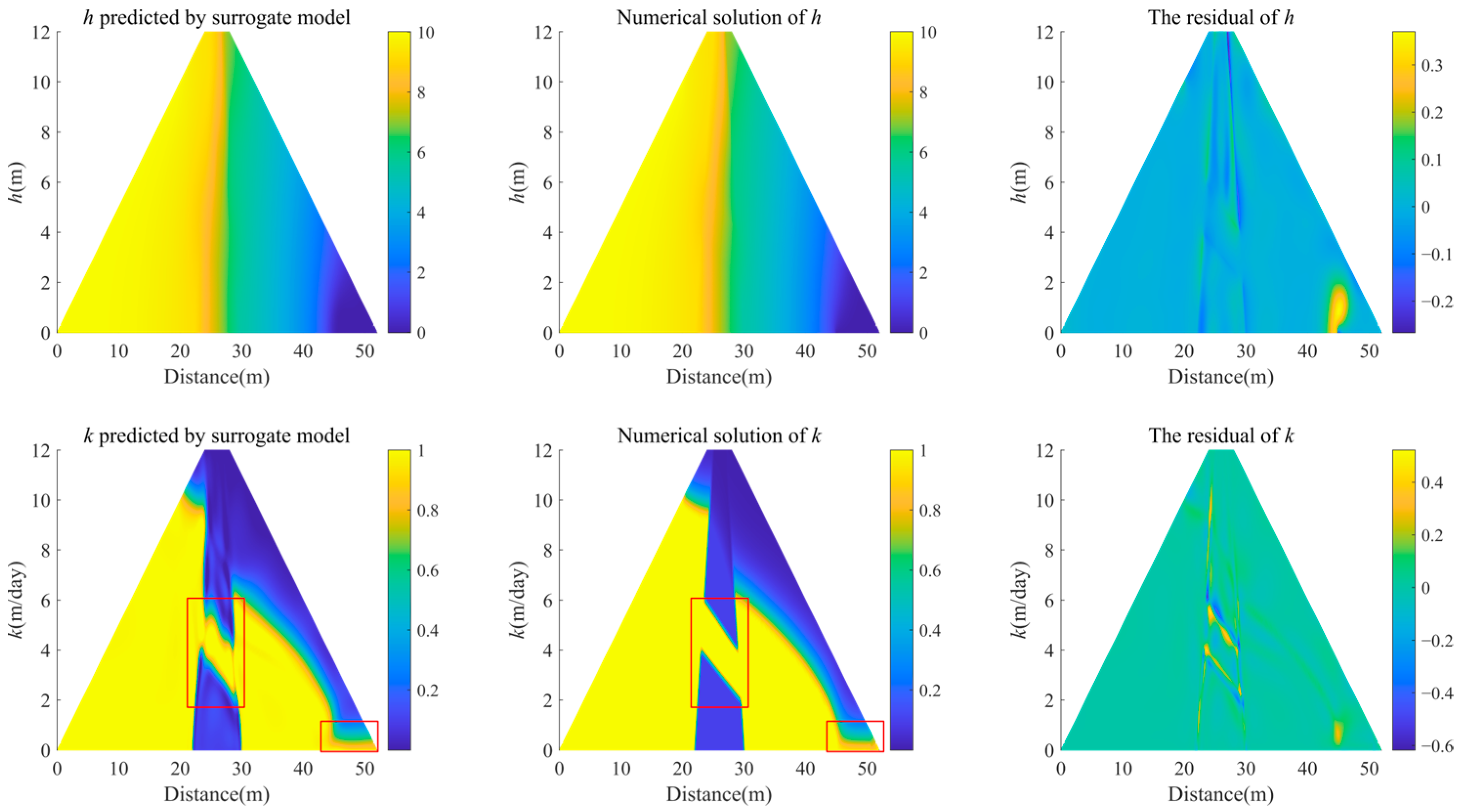
3.3. Hybrid model of trapezoidal dam

To validate the effectiveness of the proposed method in the more intuitive prediction of the seepage parameters of dams with complex structures, we investigate cases with various auxiliary structures, as reported by Lei et al. [35]. A hybrid model of a trapezoidal dam, which contains a core wall and drainage and leakage channels, was designed. In the preceding two sections, the training approach for surrogate models involved joint training using the Adam optimization algorithm and the L-BFGS optimization algorithm. However, this method’s training points were randomly chosen and remained fixed in number, posing challenges in ensuring an optimal distribution of training points when dealing with complex models. Due to the large gradient changes at the boundaries of these internal structures, in order to obtain more accurate prediction results, the RAR method is used, and the $\epsilon$ of the RAR method is set to 0.012. There are a total of 9665 points in the research domain. We randomly sample 950 points as the observed data (this includes sampling 8% of points in areas where leaks may exist). During the neural network training, we randomly sample 2048 points within the research domain and 400 points on the boundaries as the training points.

Figure 12 presents the results obtained through the combination of the Adam and L-BFGS optimization algorithms for joint training, while Figure 13 illustrates the enhanced training achieved by integrating the RAR method with the two optimization algorithms.

By comparing and analyzing Figure 12 and Figure 13, it can be found that incorporating the RAR algorithm in the training process proves to be quite beneficial for complex cases of predicting the location and shape of the drainage, the seepage channel, the core wall, and especially for quantitatively estimating the values of the seepage parameter. And the residual distribution is concentrated in a smaller range (Figure 14). The added points (black dots) are quite close to the sharp interface, which indicates the effectiveness of the RAR method. For the complex model, while the addition of training points during the training process can cause oscillation of the loss curve since the added training points may have a large error, this has no negative impact on the final prediction results (

Table 3. The L₂ relative error between the prediction results of the hybrid model of trapezoidal dam and the numerical solution (each method is calculated independently five times).

	L2 Relative Error of h	L2 Relative Error of k
Adam, L-BFGS	0.0052	0.0538
Adam, L-BFGS, and RAR	0.0040	0.0489

).

It is also observed that PINNs perform better performance in learning the spatial distribution of h compared to k, as the spatial distribution of h is relatively simpler. As the complexity of the model increases, there is a corresponding increase in the L₂ relative error. This relevance can be attributed to the rapid gradient changes in hydrologic parameters from the internal structure boundary to the background, leading to larger prediction errors for the surrogate model.

Figure 15 illustrates the convergence curves of the training process by comparing the effects of two different training strategies on the convergence of the loss function. The results indicate that the first strategy yields higher loss function values compared to the second strategy at the end of network training.

When using the RAR method for training, the training process benefits from a better distribution of training points at locations where the gradient of the seepage parameter changes rapidly. This leads to an encouraging convergence and further reduction in the value of the loss function, as shown in Figure 15, which ultimately improves the prediction accuracy of the surrogate model.

4. Conclusions

This work focuses on the seepage data assimilation of unsaturated earth–rockfill dams and develops a PINNs framework to reduce reliance on numerical models with sparse observation data. The results demonstrate that the method proposed in this paper can accurately predict hydrological parameters even with sparse observation data, yielding commendable outcomes.

In this framework, the governing equation of the seepage, the boundary conditions, and the observation data are incorporated into the loss function as hybrid constraints. To minimize the impact of rapid gradient changes in seepage parameters within the research domain, the RAR algorithm is employed to generate a proper distribution with high residuals of the PDEs for accuracy assurance.

In particular, the prediction results obtained by the proposed framework meet both the specified physical laws and the boundary conditions. This scheme has the potential to eliminate the necessity of grid subdivision or numerical discretization. It also avoids the computational overhead associated with extensive matrix operations in forward calculations, which reduces the computational complexity. It is worth mentioning that the computational burden of the trained network with a surrogate model is minimal since it does not depend on the quantity of training datasets. It is possible to predict the seepage parameters for the entire research domain with only a small amount of observation data. The proposed methodology could offer a more cost-effective alternative solution compared to data-driven deep learning methods.

This study investigates and compares the influence of three different training strategies on the prediction accuracy of the surrogate model. It can be concluded that incorporating the RAR algorithm into the joint training of both Adam and L-BFGS optimization algorithms leads to improved convergence of the loss function, as well as enhanced prediction accuracy. Furthermore, this study also explores the impact of the number of observation points on the prediction accuracy. The results demonstrate that increasing the number of observation points contributes to reducing the prediction error; however, over-reliance on observation data could lead to increased exploration costs.

References

1. Chen, S.; He, Q.; Cao, J. Seepage simulation of high concrete-faced rockfill dams based on generalized equivalent continuum model. Water Sci. Eng. 2018, 11, 250–257. [Google Scholar] [CrossRef]
2. Feng, R.; Fourtakas, G.; Rogers, B.D.; Lombardi, D. A general smoothed particle hydrodynamics (SPH) formulation for coupled liquid flow and solid deformation in porous media. Comput. Methods Appl. Mech. Eng. 2024, 419, 116581. [Google Scholar] [CrossRef]
3. Yang, Y.; Sun, G.; Zheng, H. Modeling unconfined seepage flow in soil-rock mixtures using the numerical manifold method. Eng. Anal. 2019, 108, 60–70. [Google Scholar] [CrossRef]
4. Zhang, J.; Zeng, L.; Chen, C.; Chen, D.; Wu, L. Efficient B ayesian experimental design for contaminant source identification. Water Resour. Res. 2015, 51, 576–598. [Google Scholar] [CrossRef]
5. Hou, J.; Zhou, K.; Zhang, X.; Kang, X.; Xie, H. A review of closed-loop reservoir management. Pet. Sci. 2015, 12, 114–128. [Google Scholar] [CrossRef]
6. Evensen, G. Sequential data assimilation with a nonlinear quasi-geostrophic model using Monte Carlo methods to forecast error statistics. J. Geophys. 1994, 99, 10143–10162. [Google Scholar] [CrossRef]
7. Seo, M.G.; Kim, H.M. Effect of meteorological data assimilation using 3DVAR on high-resolution simulations of atmospheric CO2 concentrations in East Asia. Atmos. Pollut. Res. 2023, 14, 101759. [Google Scholar] [CrossRef]
8. Musuuza, J.L.; Crochemore, L.; Pechlivanidis, I.G. Evaluation of earth observations and in situ data assimilation for seasonal hydrological forecasting. Water Resour. Res. 2023, 59, e2022WR033655. [Google Scholar] [CrossRef]
9. Maschio, C.; Avansi, G.D.; Schiozer, D.J. Data Assimilation Using Principal Component Analysis and Artificial Neural Network. SPE Reserv. Eval. Eng. 2023, 26, 795–812. [Google Scholar] [CrossRef]
10. Xu, Q.; Li, B.; McRoberts, R.E.; Li, Z.; Hou, Z. Harnessing data assimilation and spatial autocorrelation for forest inventory. Remote Sens. Environ. 2023, 288, 113488. [Google Scholar] [CrossRef]
11. Beven, K.; Binley, A. The future of distributed models: Model calibration and uncertainty prediction. Hydrol. Process. 1992, 6, 279–298. [Google Scholar] [CrossRef]
12. WK Hastings. Monte Carlo sampling methods using Markov chains and their applications. Biometrika 1970, 57, 97–109. [Google Scholar] [CrossRef]
13. Yeh TC, J.; Liu, S. Hydraulic tomography: Development of a new aquifer test method. Water Resour. Res. 2000, 36, 2095–2105. [Google Scholar]
14. Field, G.; Tavrisov, G.; Brown, C.; Harris, A.; Kreidl, O.P. Particle filters to estimate properties of confined aquifers. Water Resour. Manag. 2016, 30, 3175–3189. [Google Scholar] [CrossRef]
15. Zheng, Q.; Xu, W.; Man, J.; Zeng, L.; Wu, L. A probabilistic collocation based iterative Kalman filter for landfill data assimilation. Adv. Water Resour. 2017, 109, 170–180. [Google Scholar] [CrossRef]
16. Man, J.; Zheng, Q.; Wu, L.; Zeng, L. Adaptive multi-fidelity probabilistic collocation-based Kalman filter for subsurface flow data assimilation: Numerical modeling and real-world experiment. Stoch. Environ. Res. Risk Assess. 2020, 34, 1135–1146. [Google Scholar] [CrossRef]
17. Golmohammadi, M.; Harati Nejad Torbati, A.H.; Lopez de Diego, S.; Obeid, L.; Picone, J. Automatic analysis of EEGs using big data and hybrid deep learning architectures. Front. Hum. Neurosci. 2019, 13, 76. [Google Scholar] [CrossRef] [PubMed]
18. Hailesilassie, T. Rule extraction algorithm for deep neural networks: A review. arXiv 2016, arXiv:1610.05267. [Google Scholar]
19. Zhang, J.; Li, C.; Jiang, W.; Wang, Z.; Zhang, L.; Wang, X. Deep-learning-enabled microwave-induced thermoacoustic tomography based on sparse data for breast cancer detection. IEEE Trans. Antennas Propag. 2022, 70, 6336–6348. [Google Scholar] [CrossRef]
20. Mao, B.; Han, L.; Feng, Q.; Yin, Y. Subsurface velocity inversion from deep learning-based data assimilation. J. Appl. Geophys. 2019, 167, 172–179. [Google Scholar] [CrossRef]
21. Tang, M.; Liu, Y.; Durlofsky, L.J. A deep-learning-based surrogate model for data assimilation in dynamic subsurface flow problems. J. Comput. Phys. 2020, 413, 109456. [Google Scholar] [CrossRef]
22. Tang, M.; Liu, Y.; Durlofsky, L.J. Deep-learning-based surrogate flow modeling and geological parameterization for data assimilation in 3D subsurface flow. Comput. Methods Appl. Mech. Eng. 2021, 376, 113636. [Google Scholar] [CrossRef]
23. Kang, X.; Kokkinaki, A.; Power, C.; Kitanidis, P.; Shi, X.; Duan, L.; Liu, T.; Wu, J. Integrating deep learning-based data assimilation and hydrogeophysical data for improved monitoring of DNAPL source zones during remediation. J. Hydrol. 2021, 601, 126655. [Google Scholar] [CrossRef]
24. Sun, L.; Gao, H.; Pan, S.; Wang, J. Surrogate modeling for fluid flows based on physics-constrained deep learning without simulation data. Comput. Methods Appl. Mech. Eng. 2020, 361, 112732. [Google Scholar] [CrossRef]
25. Raissi, M.; Perdikaris, P.; Karniadakis, G.E. Physics-informed neural networks: A deep learning framework for solving forward and inverse problems involving nonlinear partial differential equations. J. Comput. Phys. 2019, 378, 686–707. [Google Scholar] [CrossRef]
26. Chen, Y.; Lu, L.; Karniadakis, G.E.; Dal Negro, L. Physics-informed neural networks for inverse problems in nano-optics and metamaterials. Opt. Express. 2020, 28, 11618–11633. [Google Scholar] [CrossRef] [PubMed]
27. Xue, L.; Dai, C.; Han, J.X.; Yang, M.; Liu, Y. Deep neural network model driven jointly by reservoir seepage physics and data. Pet. Geol. Recovery Effic. 2020, 29, 145–151. [Google Scholar]
28. Tartakovsky, A.M.; Marrero, C.O.; Perdikaris, P.; Tartakovsky, G.D.; Barajas-Solano, D. Physics-informed deep neural networks for learning parameters and constitutive relationships in subsurface flow problems. Water Resour. Res. 2020, 56, e2019WR026731. [Google Scholar] [CrossRef]
29. He, Q.; Barajas-Solano, D.; Tartakovsky, G.; Tartakovsky, A. Physics-informed neural networks for multiphysics data assimilation with application to subsurface transport. Adv. Water Resour. 2020, 141, 103610. [Google Scholar] [CrossRef]
30. Zhang, S.; Lan, P.; Su, J.; Xiong, H. Simulation and parameter identification of groundwater flow model based on PINNs algorithms. Chin. J. Geotech. Eng. 2023, 45, 376–383. [Google Scholar]
31. Depina, I.; Jain, S.; Mar Valsson, S.; Gotovac, H. Application of physics-informed neural networks to inverse problems in unsaturated groundwater flow. Georisk 2022, 16, 21–36. [Google Scholar] [CrossRef]
32. Shadab, M.A.; Luo, D.; Hiatt, E.; Shen, Y.; Hesse, M.A. Investigating steady unconfined groundwater flow using Physics Informed Neural Networks. Adv. Water Resour. 2023, 177, 104445. [Google Scholar] [CrossRef]
33. Yang, Y.; Gong, H.; Zhang, S.; Yang, Q.; Chen, Z.; He, Q.; Li, Q. A data-enabled physics-informed neural network with comprehensive numerical study on solving neutron diffusion eigenvalue problems. Ann. Nucl. Energy 2023, 183, 109656. [Google Scholar] [CrossRef]
34. Lu, L.; Meng, X.; Mao, Z.; Karniadakis, G.E. DeepXDE: A deep learning library for solving differential equations. SIAM Rev. Soc. Ind. Appl. Math. 2021, 63, 208–228. [Google Scholar] [CrossRef]
35. Lei, Y.; Dai, Q.; Zhang, B.; Zhou, W.; Yang, J. Saturated-unsaturated seepage simulation and hydrological dam models for quantifying the heterogeneity to hydrological state variables: Impacts of auxiliary structures and leakage anomalies. Int. J. Numer. Anal. Methods Geomech. 2023, 47, 2064–2084. [Google Scholar] [CrossRef]
36. Richards, L.A. Capillary conduction of liquids through porous mediums. Physics 1931, 1, 318–333. [Google Scholar] [CrossRef]
37. Van Genuchten, M.T. A closed-form equation for predicting the hydraulic conductivity of unsaturated soils. Soil Sci. Soc. Am. J. 1980, 44, 892–898. [Google Scholar] [CrossRef]
38. Glorot, X.; Bengio, Y. Understanding the difficulty of training deep feedforward neural networks. In Proceedings of the Thirteenth International Conference on Artificial Intelligence and Statistics, Sardinia, Italy, 13–15 May 2010; pp. 249–256. [Google Scholar]
39. Baydin, A.G.; Pearlmutter, B.A.; Radul, A.A.; Siskind, J.M. Automatic differentiation in machine learning: A survey. J. Mach. Learn. Res. 2018, 18, 1–43. [Google Scholar]
40. Abadi, M.; Barham, P.; Chen, J.; Chen, Z.; Davis, A.; Dean, J.; Devin, M.; Ghemawat, S.; Irving, G.; Isard, M.; et al. Tensorflow: A system for large-scale machine learning. In Proceedings of the 12th USENIX Symposium on Operating Systems Design and Implementation (OSDI 16), Savannah, GA, USA, 2–4 November 2016. [Google Scholar]
41. Paszke, A.; Gross, S.; Chintala, S.; Chanan, G.; Yang, E.; DeVito, Z.; Lin, Z.; Desmaison, A.; Antiga, L.; Lerer, A. Automatic differentiation in pytorch. In Proceedings of the 31th Annual Conference on Neural Information Processing Systems (NIPS 2017), Long Beach, CA, USA, 4–9 December 2017. [Google Scholar]
Figure 1. Schematic diagram of saturated–unsaturated seepage in an earth–rockfill dam.
Water 16 01041 g001
Figure 2. Schematic diagram of seepage field data assimilation based on PINNs: the left is the architecture of fully connected neural network; the middle is the hybrid constraints composed of PDEs, boundary conditions, and observation points; the right is the optimal neural network parameters obtained after optimization training.
Water 16 01041 g002
Figure 3. Training process of the proposed neural network model.
Water 16 01041 g003
Figure 4. Homogeneous rectangular dams: surrogate model predictions compared with numerical solutions.
Water 16 01041 g004
Figure 5. L2 relative error varies with different numbers of observation points.
Water 16 01041 g005
Figure 6. Convergence curve of the training process for the homogeneous rectangle dam.
Water 16 01041 g006
Figure 7. Residual distributions of the homogeneous rectangular dam: (a) residual distribution of h and (b) residual distribution of k.
Water 16 01041 g007
Figure 8. Homogeneous trapezoidal dam: surrogate model predictions compared with numerical solutions.
Water 16 01041 g008
Figure 9. Trapezoidal dam with core wall: surrogate model predictions compared with numerical solutions.
Water 16 01041 g009
Figure 10. Residual distributions: (a) residual distribution of h for homogeneous trapezoidal dam; (b) residual distribution of k for homogeneous trapezoidal dam; (c) residual distribution of h for trapezoidal dam with core wall; (d) residual distribution of k for trapezoidal dam with core wall.
Water 16 01041 g010
Figure 11. Convergence curves of the training process: (a) homogeneous trapezoidal dam and (b) trapezoid dam with core wall.
Water 16 01041 g011
Figure 12. Hybrid model of trapezoidal dam: surrogate model predictions compared with numerical solutions (Adam and L-BFGS). The red box shows the location of leakage channels and drainage.
Water 16 01041 g012
Figure 13. Hybrid model of trapezoidal dam: surrogate model predictions compared with numerical solutions (Adam, L-BFGS, and RAR). The red box shows the location of leakage channel and drainage.
Water 16 01041 g013
Figure 14. Residual distributions of hybrid model of trapezoidal dam: (a) residual distribution of h (Adam and L-BFGS); (b) residual distribution of k (Adam and L-BFGS); (c) residual distribution of h (Adam, L-BFGS, and RAR); (d) residual distribution of k (Adam, L-BFGS, and RAR).
Water 16 01041 g014
Figure 15. Convergence curves of the training process for Model 3: (a) Adam and L-BFGS and (b) Adam, L-BFGS, and RAR.
Water 16 01041 g015