Abstract
The jar test is the current standard method for predicting the performance of a conventional drinking water treatment (DWT) process and optimizing the coagulant dose. This test is time-consuming and requires human intervention, meaning it is infeasible for making continuous process predictions. As a potential alternative, we developed a machine learning (ML) model from historical DWT plant data that can operate continuously using real-time sensor data without human intervention for predicting clarified water turbidity 15 min in advance. We evaluated three types of models: multilayer perceptron (MLP), the long short-term memory (LSTM) recurrent neural network (RNN), and the gated recurrent unit (GRU) RNN. We also employed two training methodologies: the commonly used holdout method and the theoretically correct blocked cross-validation (BCV) method. We found that the RNN with GRU was the best model type overall and achieved a mean absolute error on an independent production set of as low as 0.044 NTU. We further found that models trained using BCV typically achieve errors equal to or lower than their counterparts trained using holdout. These results suggest that RNNs trained using BCV are superior for the development of ML models for DWT processes compared to those reported in earlier literature.
1. Introduction
In a conventional drinking water treatment (DWT) plant, the unit processes of coagulation and flocculation, followed by clarification and filtration, are primarily responsible for removing large colloidal particles and natural organic matter from water [1]. The success of these downstream processes depends on the effective agglomeration of particles into flocs in the upstream coagulation and flocculation processes. Floc formation is affected not only by coagulant and flocculant addition but also by several raw water quality parameters, including conductivity, initial turbidity, and initial suspended-solids concentration [2], which are often prone to rapid fluctuations due to climatic events. Temperature and pH have a particularly significant influence on this process as they affect coagulant hydrolysis, flocculation kinetics, coagulant speciation, organic matter adsorption, and charge neutralization [3].
Due to the complex nature of the coagulation process, there is no mathematical model as of yet that accounts for all of the relevant parameters that can be used to accurately predict the behavior of the coagulation process [2], especially for natural waters for which organic matter reactivity remains poorly defined. As a result, the jar test [4] remains the standard method of testing coagulation behavior and estimating optimal coagulant addition. The jar test is performed at bench scale. It involves adding various coagulant doses to a raw water sample at various pH levels and measuring the settling behavior and resulting turbidity. Despite its ubiquity, the jar test has some drawbacks. The need for an operator to manually perform lab tests means that there is an appreciable labor requirement associated with this procedure. Additionally, the water sample upon which the test is performed is taken at a single point in time. In contrast, a treatment plant’s influent water quality constantly changes based on the season and weather events. For this reason, jar testing cannot be used to continuously optimize a coagulation process as raw water quality often changes too quickly for this to be feasible [2]. As a result, jar test results do not necessarily translate well to full-scale operation, and scaling up the jar test conditions to various full-scale processes is a common challenge.
To overcome the limitations of the jar test and improve the operational predictions, we investigated the potential to use continuous sensor data to predict clarified water turbidity. Online water quality sensors are available to automatically and continuously measure and record most of the relevant water quality and operational parameters affecting the coagulation, flocculation, and clarification processes [2]. One such sensor in some DWT plants is the streaming current detector (SCD), which measures the surface charge on solid particles in the coagulation basin [5]. While it is possible to develop a control loop that attempts to maintain zero net charge on the particles in the coagulation basin using the SCD, the set points for various raw water conditions are still determined via jar testing or empirically based on the performance of the full-scale process [6]. As demonstrated by the authors in [5], such control loops can also be unstable as plants can adjust both pH and coagulant dose independently, which both affect streaming current readings. While they developed a model in which pH and coagulant dose can be somewhat decoupled through an estimated relationship between pH and SCD measurements, they acknowledge that their analysis indicates that other variables contribute an appreciable amount of variability to the data that are not considered in their model.
Some authors have developed empirical feedforward control models to predict optimal operating conditions based on measures of raw water quality [7,8]. These models can vary widely in complexity and serve to identify which coagulant results in optimal settled water quality based on one or more raw water quality parameters. While these models may serve as a useful starting point for operators to determine a good coagulant dose, they face some issues. Notably, these empirical models require lots of manual work and are prone to the inductive biases of the authors that develop them based on their assumptions of the data distribution and importance of certain variables. Perhaps the most notable drawback is that such a model is difficult to update if the quality of the source water feeding the plant changes significantly, as the entire modelling process must essentially be repeated. This concern is increasingly relevant as climate change is causing the degradation of source water quality due to exaggerated wet and dry periods [9], increased erosion caused by wildfires [10], and the disruption of seasonal phenomena [11]. These effects can lead to more frequent turbidity spikes which render drinking water treatment more difficult [12,13], in addition to continuously rendering models based on old water quality data obsolete.
Another means of leveraging continuous sensor data to aid in process control is through the use of machine learning (ML). ML models typically require a large amount of historical data in order to be developed, and nowadays many DWT plants have enough archived operating data for ML model development to be feasible. These ML models can be automatically re-trained as new data becomes available in order to continuously keep them applicable to current conditions. The goal of an ML model is to establish a relationship between observed input and output data, without necessarily having to mathematically explain the underlying phenomenon, which makes this an appropriate method to apply to the coagulation process. Interest in applying ML to the DWT industry is not new; in fact, there is a sizable body of existing research in this field. Much of this work involved investigating the potential of applying artificial neural networks (ANNs), a type of ML model, to aid with DWT process control of the conventional water treatment process using historical plant operating data. Examples of these previous studies include: predicting the filtered water turbidity in LaVerne, California, USA [14]; predicting the clarified water quality and optimal alum dose in Union, Ontario, Canada [15]; predicting the optimal coagulant dose at a plant in Brazil [16]; predicting the optimal alum dose in Sabah, Malaysia [17]; and predicting the optimal PID control elements for a coagulant dosing pump at a treatment plant [18].
In much of the previous research, such as the studies listed above, the authors use the multilayer perceptron (MLP) model to make predictions of future values based on previous ones. However, the MLP model has no mechanisms to treat information sequentially. This is in contrast to recurrent neural networks (RNNs), which are specialized for processing sequential data [19]; they should perform better than MLPs for time series problems in DWT. Additionally, we note that these previous studies employ the holdout method for model evaluation. This method involves shuffling the data before splitting it into training/validation/testing subsets, which, for time series data, can lead to the phenomenon of “data leakage.” This can bias the model’s evaluation, leading to an inflated estimate of the model’s performance and a suboptimal final model [20]. We compare this to an alternate training methodology explicitly developed for sequential data known as blocked cross-validation (BCV) [21,22]. BCV keeps the data in its sequential order to avoid potential data leakage and additionally increases the proportion of the data available for model training, which can result in the model having better predictive capabilities.
The remainder of this paper is structured as follows. Section 2 explains the methodology, which includes the preparation of the data, model implementation, choice of model types, and model training and testing. Section 3 contains an analysis of the results, which includes a comparison of the performance of the different types of models and comparing the two different model training methodologies. Section 4 is a discussion of these results, including their implications for authors wishing to model time series data and further research that can be performed to build upon these results.
2. Methodology
2.1. Data Analysis and Preprocessing
The data set for this research project comes from the Chomedey drinking water treatment plant in Laval, Québec, Canada. This plant collects surface water from Des Prairies River in an area where most of the adjacent land use on the riverbanks is suburban residential. From 1981 to 2010, the area experienced an average annual rainfall of 785 mm, an average annual snowfall of 210 cm, and average temperatures climbing above freezing in April [23]. This combination of heavy snowfall followed by warmer temperatures in spring makes the river prone to significant freshets in the spring. The treatment process at this plant consists of screening, coagulation, flocculation, clarification, ozonation, biological filtration, and disinfection; for this study, we examined only the coagulation, flocculation, and clarification processes. These processes occur in three parallel Actiflo® HCS (high concentration sludge) clarifiers [24], of which two usually are in operation at any given time. The plant typically uses alum as a coagulant and cationic polyacrylamide as a flocculant.
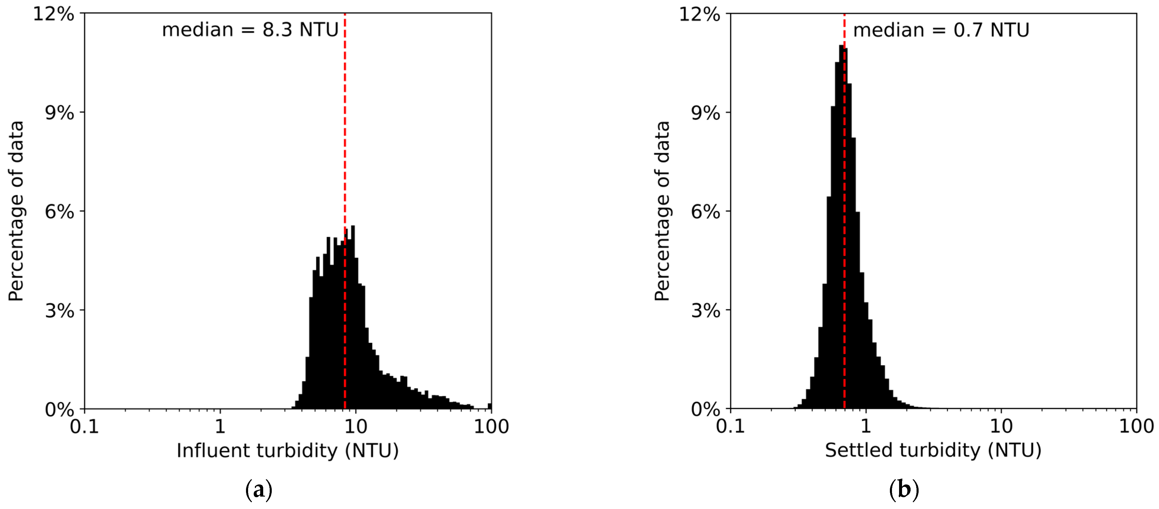
The plant data set originates from online sensors collected at one-minute intervals from July 2017 to November 2021 for 2,243,440 data points. Note that each data point contains operating information for, on average, two active clarifiers. We use seven variables for model development: influent turbidity, influent temperature, influent conductivity, coagulation basin pH, alum dosage, flow rate, and clarified turbidity. Data were removed where values were missing or suspected to be erroneous, resulting either from frozen sensor values (suggesting a communication issue between the sensor and the control software) or from momentary spikes or drops in sensor values that quickly returned to normal (suggesting some noise). After these changes, the data set was reduced by 9.91% to 2,021,104 data points. A histogram illustrating the distribution of clarified water turbidity values in the cleaned data set is presented below in Figure 1.
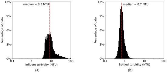
Figure 1.
Empirical distribution of the plant’s turbidity in the (a) influent water and (b) settled water.
All the variables are then scaled to a range of [0,1] using the minimum and maximum value of each variable in the data set according to Equation (1):
One of the variables that we omitted from our model development is the polymer dose. While polymer addition is critical to the success of the Actiflo® process, in this data set, polymer dose data are only available from September 2020 onwards. Since data quantity is critical for developing ML models, especially for those modelling seasonal phenomena, including the polymer dose in our model would severely limit the model quality. Some experiments comparing identical model architectures trained with and without the inclusion of the polymer dose using a truncated version of the data from September 2020 onwards revealed no statistically significant difference in model performance with or without the polymer dose. This is likely due to the low variability in polymer dose values across the data set, as it is already well optimized, which means that this variable imparts little additional information to the model. Dissolved organic carbon (DOC) is not included as an input to our model as the plant does not have any continuous sensors for measuring influent DOC concentration. While DOC does typically have an effect on the performance of the coagulation process, it is relatively stable in this area of the Des Prairies River throughout the year (mean = 6.2 mg/L, standard deviation = 0.7 mg/L) [25] and therefore the plant’s coagulation process is dictated by optimizing for turbidity removal. The addition of a DOC sensor in the future may be useful to improve model performance, but this difference should not be significant.
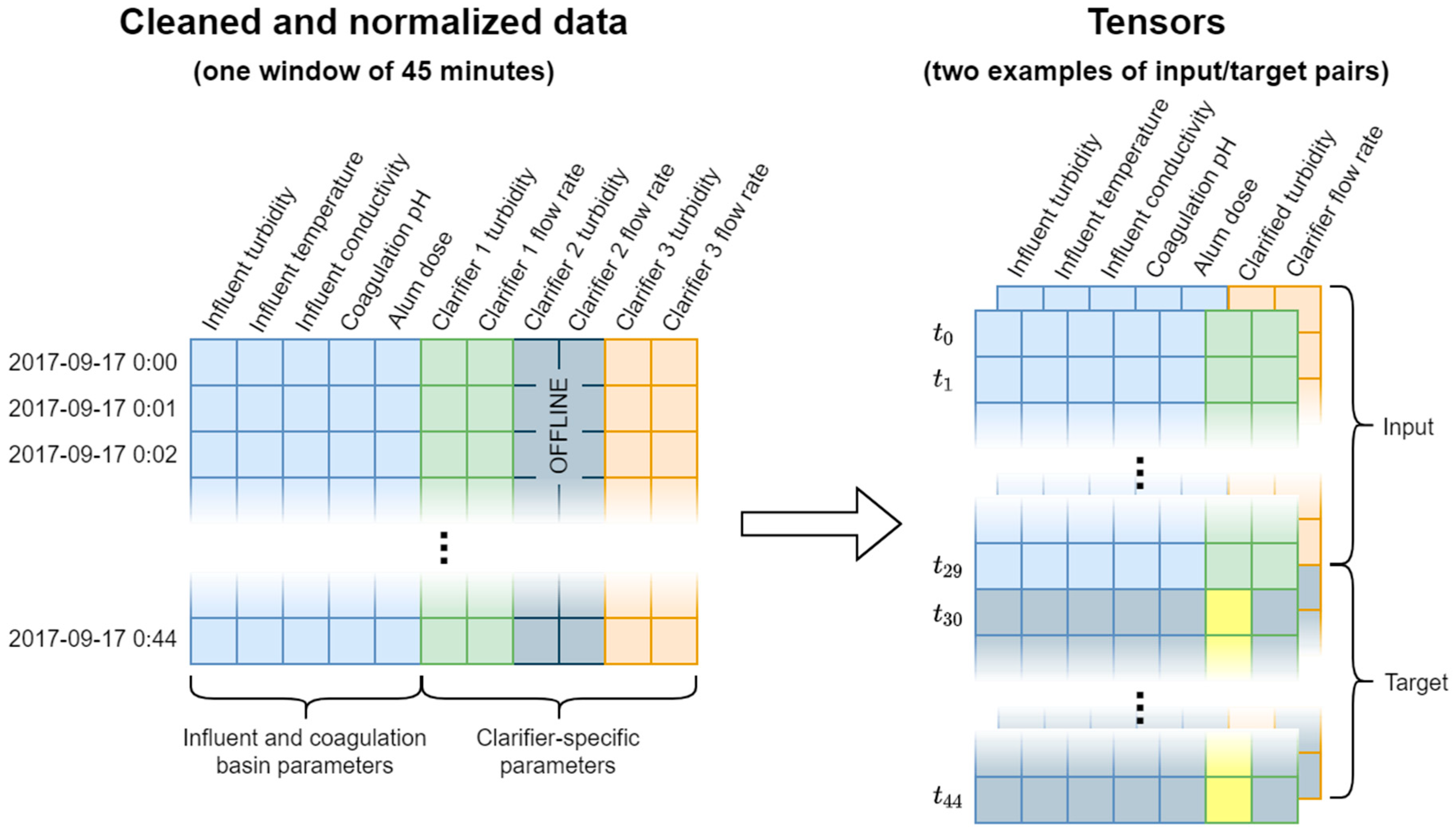
The raw data are converted into a tensor for model training and evaluation. We applied overlapping sliding windows that are 45-time steps in length to create individual examples to include in the tensor. Since flow rate and clarified turbidity are recorded per clarifier, we make multiple examples of the data at each time step that share the five common variables (influent turbidity, influent temperature, influent conductivity, coagulation basin pH, and alum dose) with the unique flow rate and clarified water turbidity for each online clarifier. Each example in the tensor is therefore a 45 × 7 matrix, representing 45 consecutive minutes of measured values for the 7 variables outlined above. Each 45-min data window is turned into two examples, one per active clarifier. The first 30 min of the data includes all variables and is used as input to the model; the last 15 min of the data includes only the clarified turbidity and is the target for the model to predict. Since this approach requires 45 consecutive data points, many examples are removed as they contain an isolated time step that is missing data. This results in a total of 1,539,890 examples in the final data set. This process is summarized visually in Figure 2.
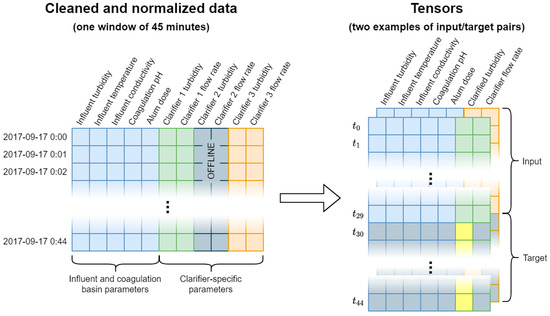
Figure 2.
Illustration of the process of turning the raw data into tensors.
2.2. Implementation
The model receives as input 30 time steps (30 min) of data for all 7 variables described previously, and its task is to predict the evolution of the clarified water turbidity over the next 15 time steps (15 min). These values were selected as the hydraulic retention time (HRT) in the Actiflo® basin at the design capacity is roughly 13 min. Therefore, we provided the model with roughly two HRTs of data as input and tasked it with predicting the effluent approximately one HRT in advance, which should be solely a function of what can already be measured in the system at that time. The model error is calculated as the root-mean-square error (RMSE) during training, according to Equation (2):
where is the true value of data point i, is the corresponding value predicted by the model, and N is the total number of data points in the set. In the text however, we report errors as mean absolute error (MAE) as this measure is more intuitive, according to Equation (3):
The results are passed through the inverse of the normalization function applied to the clarified turbidity variable before the error is calculated, such that the reported error is in the original units of NTU. All programming was performed in Python using the PyTorch package. The code we developed for model training and evaluation can be found in the Supplementary Materials. Training was performed locally using an Nvidia GeForce RTX 3080 12G GPU.
2.3. Model Selection
In Section 1 it was identified that much of the previous literature applying ML to DWT, including relatively recent studies, employs the multilayer perceptron (MLP) model. The MLP is the most standard form of ANN [19]. Thus, we employ MLP in this study to establish a baseline level of performance. The mathematical details for the MLP and all other ANN architectures are outside the scope of this paper; readers wishing to familiarize themselves with each model in detail are referred to the cited literature.
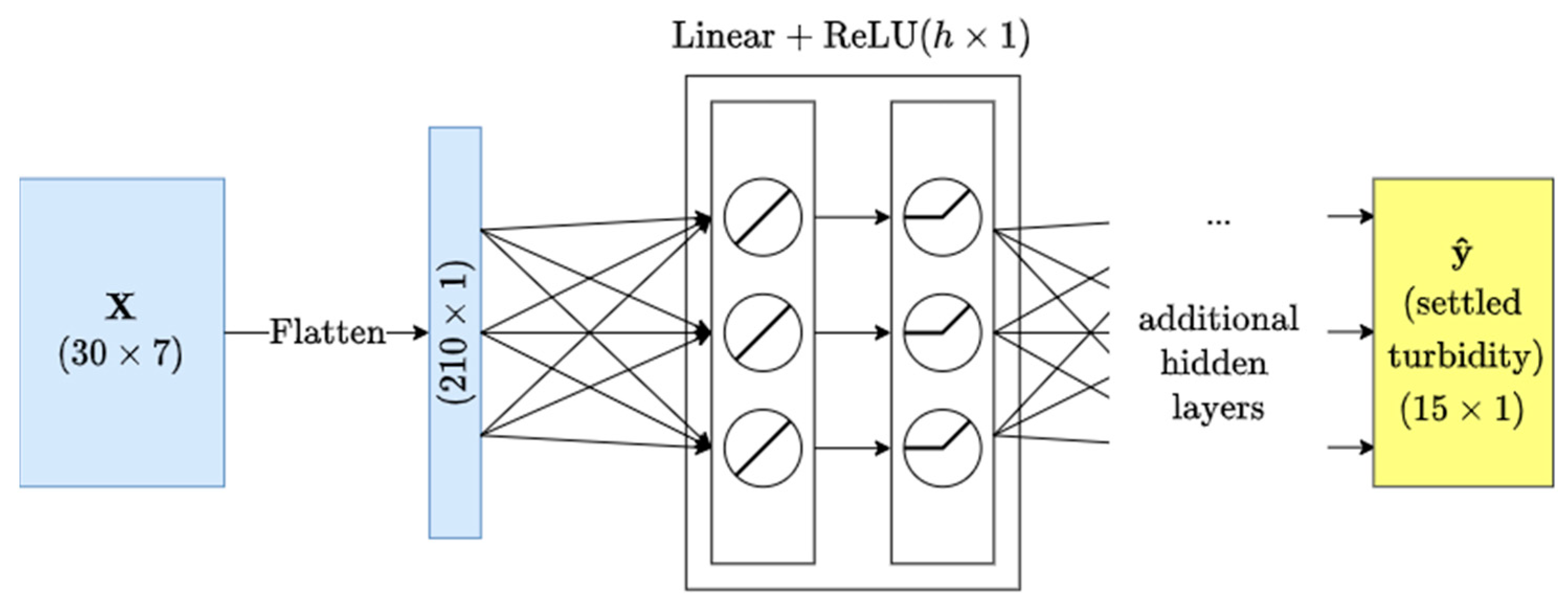
We employ an MLP where each hidden layer is composed of a linear part followed by a nonlinear ReLU part. For our MLP model only, the two-dimensional input tensor is flattened to one dimension before the first input layer. For the MLP we test a grid search of hyperparameters where the number of hidden layers is (2, 3, 4) and the number of hidden units h per layer is (960, 1920, 3840). A visual diagram of our MLP implementation is provided in Figure 3.
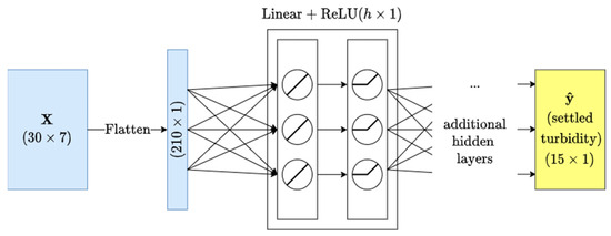
Figure 3.
Diagram of the multilayer perceptron implementation.
Given that the data used in this study are a time series, we consider two types of recurrent neural networks (RNN). The architecture of an RNN contains recurrent connections that force the network to model current data in terms of past data. This is useful in this particular situation as data points have a temporal relationship. While standard RNNs often encounter certain difficulties while training, typically referred to as the vanishing/exploding gradient problem, there exist modified RNN architectures with preferable properties that achieve better results by allowing the modelling of longer-term dependencies.
Arguably the most popular RNN architecture is the long short-term memory network, or LSTM [26]. In an LSTM network, each time step in the series is processed by a memory cell composed of three gates that control the flow of information from the current and previous time steps. This allows for more uniform error flow during backpropagation and, thus, is less prone to vanishing/exploding gradients. A similar gated architecture is the gated recurrent unit, or GRU [27]. This architecture is a modified version of the LSTM, but the cell uses two gates instead of three and, therefore, tends to train faster for a fixed number of parameters. However, it is unclear if one is superior to the other across all tasks [28].
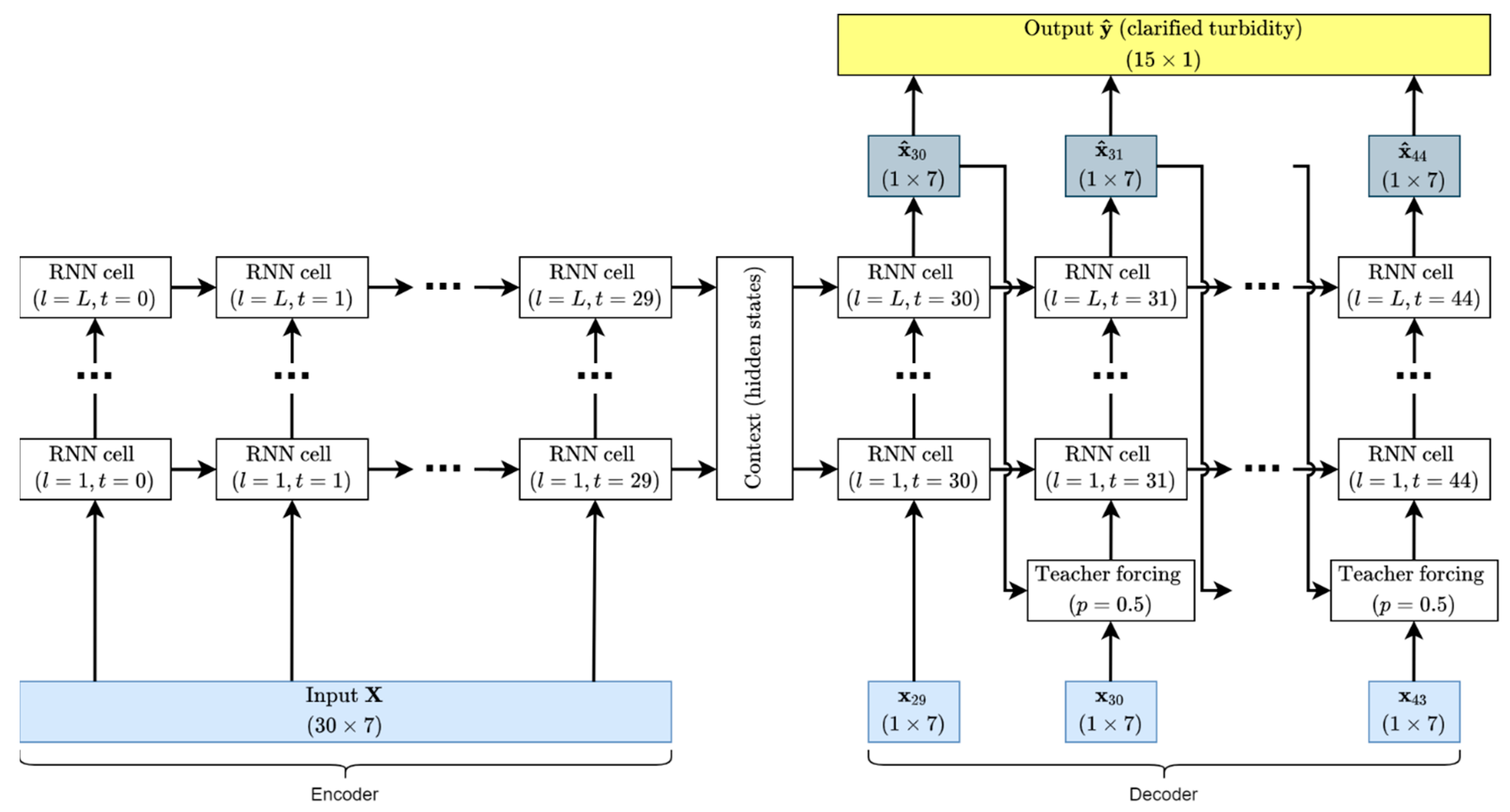
For this study, we tested the RNNs in an encoder–decoder arrangement. In our implementation, the encoder and decoder are an RNN of the same type with the same hyperparameters (number of hidden layers and hidden layer size). This arrangement first encodes the input sequence into a “context” composed of a hidden state and cell state. Each of these states is a matrix with dimensions of (number of hidden layers) × (hidden layer size). The context is then provided to the first temporal layer of the decoder RNN along with the last effluent turbidity value in the input sequence to predict the first effluent turbidity value in the output sequence. This predicted value and the new hidden and cell states are provided recursively to a new temporal RNN layer for the desired number of time steps, illustrated in Figure 4. Note that in this figure, the RNN cells are always of the same type: either LSTM or GRU. Our implementation also uses teacher forcing during training [29], in which the last predicted value may instead be replaced with the ground truth value at the next timestep with probability ; this technique tends to speed up model training by nudging the model into the correct range of output values multiple times during each training step. For both types of RNN we test a grid search of hyperparameters where the number of hidden layers is (2, 3, 4) and the number of hidden units per layer is (32, 64, 128).
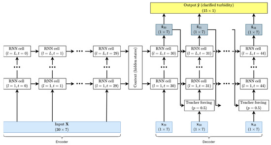
Figure 4.
Diagram of the encoder–decoder RNN implementation.
2.4. Training and Testing
In machine learning, it is common practice to employ cross-validation for optimal model selection [30]. The simplest form of cross-validation is the holdout method, which entails dividing the data randomly into three static subsets: a training set, a validation set, and a test set—a typical ratio being 50%, 25%, and 25% of the total data, respectively. The training set is used to train the model—that is, it is the data used by the computer to adjust the model’s parameters. The training process makes these adjustments to improve the model’s performance on the given task with that particular data set. Since we want the model to perform well on all possible data it might encounter during this task, we periodically assess its performance on the validation set. We use the early stopping strategy [19], which means we stop training once the model’s performance begins to degrade on the validation set, as this suggests that the model has begun to overfit to the training set and therefore no longer performs the desired task in a generalized way. The test set is only used once model training is concluded, and the model’s performance on this set gives an estimate of what the model’s performance will be once it is deployed to perform the task in a real situation. We wish to maximize the amount of data in the training set to achieve the highest model performance. Still, we must also be careful to keep the validation and test sets large enough to have good estimates of the model’s performance on data outside of its training set.
One problem that we identified in multiple previous studies applying ML to DWT is that of potential data leakage [14,15,31,32,33]. Data leakage is a situation in which a model is trained on data that it does not have access to under real circumstances [20]. In the referenced studies, the authors rearranged their data, either via a heuristic or a random shuffle, before splitting them into static subsets or folds. This introduces two potential sources of data leakage into the model. These two sources being that the model is trained on data obtained later than other data in the validation and test sets, and that data windows in the training set can overlap with data windows in the validation and test sets. In a real-life situation, our model necessarily does not have access to data in the future. This means that these models were tested in a way that does not accurately reflect their situation if deployed into real operation. Such a training paradigm can also degrade model performance as the data leakage may mean that overfitting is detected much later than if the training and validation data were held in chronological order.
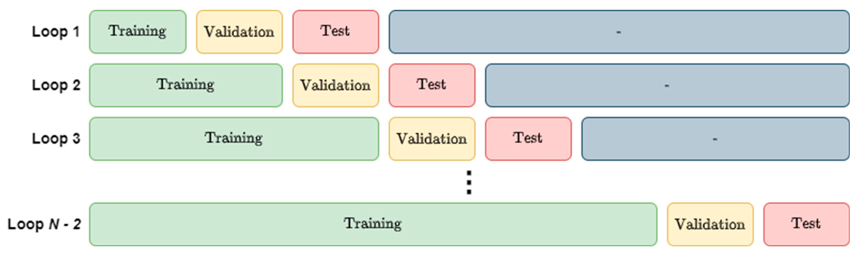
To avoid data leakage and to increase the amount of data available during training compared to using static subsets, we employed a training methodology originally proposed by Snijders [21] and referred to as “blocked cross-validation” (BCV) in [22]. With BCV, those data are not divided into static subsets, but instead these subsets change over the course of training. We start by dividing the data equally into N parts, which we will call blocks and will refer to sequentially as being blocks (1, 2, … N − 1, N). The data are always left in chronological order. We first start by using block 1 as the training set, block 2 as the validation set, and block 3 as the test set. We train the model until it converges (i.e., until the validation error begins to increase), test the model, and record the test error on block 3. We then increase the size of the training subset by 1 block such that blocks 1 and 2 are now the training set, block 3 is the validation set, and block 4 is the test set. This process repeats until block N has been used as the test set. The model’s test error is estimated as the arithmetic mean of the error on all N − 2 test blocks. This strategy is illustrated visually in Figure 5.
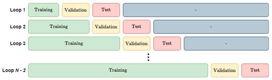
Figure 5.
Illustration of the blocked cross-validation approach.
The BCV approach should be preferred for time series data specifically since these data are not independent. Data being independent is a fundamental assumption of the holdout training method; using time series data violates that assumption [30]. BCV avoids this as we assure that data windows in each set do not overlap and are sufficiently far apart in time so as to not be dependent. In addition to avoiding data leakage in this context, BCV allows us to increase the fraction of data available in all three subsets, as most of the data can be reused in each of them. This can lead the model to converge to a better solution and reduce bias in the model performance estimate. However, it is worth noting that this renders the training process more computationally expensive than the holdout method.
In our implementation, we set N = 14, which means 12 blocks are used in each data set. This effectively results in 85% of the overall data set being used for training, validation, and testing over the entire course of training, compared to the typical 50%, 25%, and 25%, respectively, when using the holdout method. For this step, we use only data from July 2017 to July 2020, reserving the remainder for comparing the two cross-validation methods. Optimization is performed using the Adam algorithm [34] with a learning rate of 5 × 10⁻⁴, as this was determined through experimentation to result in the lowest validation model errors. We use a minibatch size of 64 as, through experimentation, it was observed to converge to better solutions than larger batch sizes while still being reasonably computationally efficient. We iterate for each of the 12 different block distributions until the validation loss has not improved for the last 10 epochs, up to a maximum of 100 epochs per training loop. We use a weight decay (L2 norm penalty on the model parameters) of 1 × 10⁻⁸ and clip gradients to a norm of 1 as these hyperparameters were observed to improve training performance.
3. Results
3.1. Model Performance
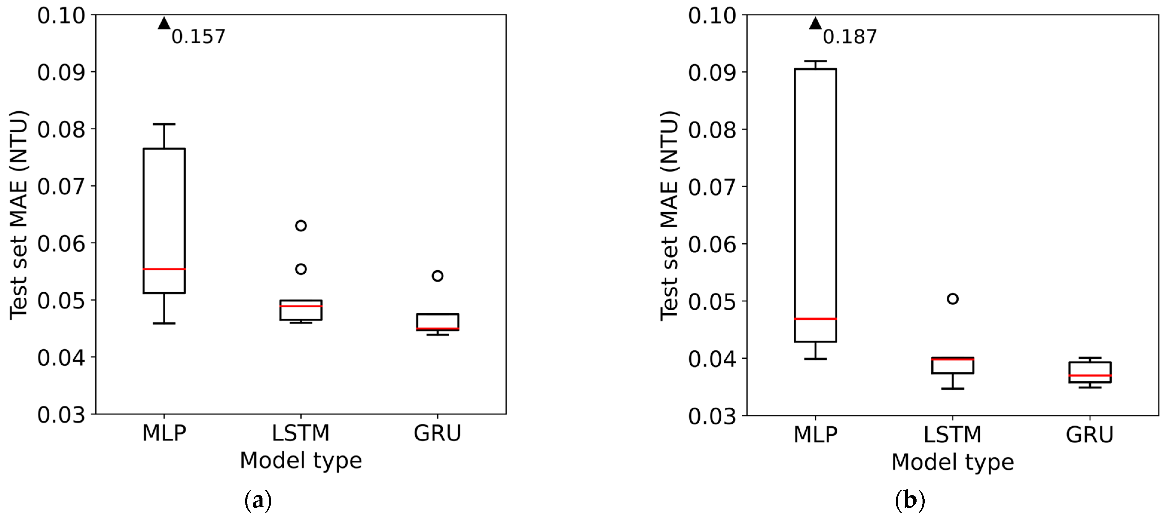
The distribution of the test set MAEs for each size of the trained model, as described in the methodology, is illustrated in Figure 6, and summary statistics are presented in Table 1 and Table 2. Note that while the y-scale for both graphs is the same, the data points in the BCV test set are not the same as the data points in the holdout test set, and therefore, the results are not directly comparable between the two graphs.
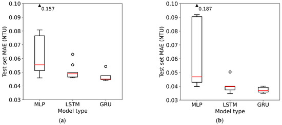
Figure 6.
Distribution of test set errors for the different sizes of each model type trained using: (a) blocked cross-validation and (b) holdout.

Table 1.
Summary statistics of test set performance for models trained using BCV.
Table 2.
Summary statistics of test set performance for models trained using holdout.
Since the two test sets are different, we cannot directly compare the results of the two training methodologies—for this we will evaluate the models on the data that we reserved for this purpose at the end of the original data set.
Regardless of the training method, similar patterns are observed in both graphs. The MLPs demonstrate considerably higher variability in model performance than the LSTMs or GRUs. This suggests that hyperparameter tuning (in terms of the number of hidden layers and hidden layer size) is less important for the RNNs than it is for MLP to find an optimal model. However, the best model in each class achieves very similar performance, with an error difference between the three best models trained using BCV and holdout of only 0.02 NTU and 0.05 NTU, respectively. It is notable, however, that GRU consistently has the lowest overall and median errors in both cases.
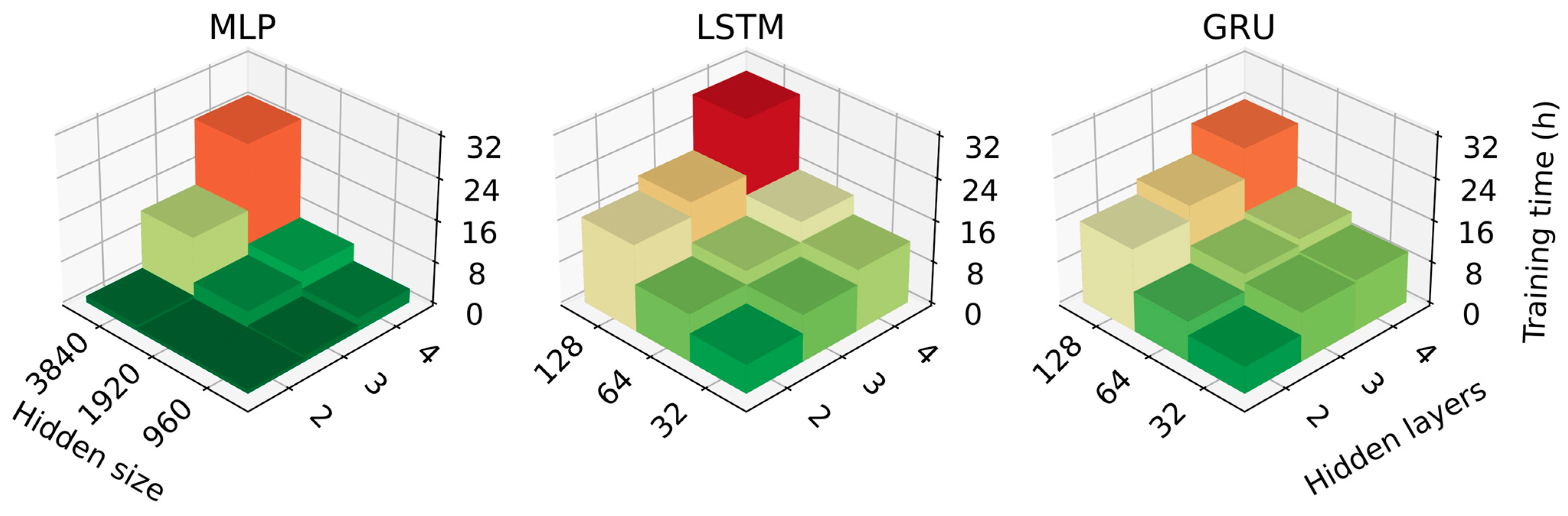
While training time does not affect model performance when used in production, it is helpful to know how the training time scales with model size for instances with limited training budget. The training time using BCV for each size of the model is presented in Figure 7.
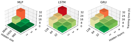
Figure 7.
Total training time using blocked cross-validation for each of the implemented models.
It is notable in the above figure that small MLPs train notably faster than small LSTMs and GRUs. However, as model size increases, this advantage begins to diminish, and in the case of the largest models we trained, GRU had a slightly shorter training time for MLP. This suggests that for larger models than those used here, MLPs would have very long training times, which, coupled with the fact that they also require more hyperparameter tuning, may make them infeasible in such a case.
3.2. Cross-Validation Methods
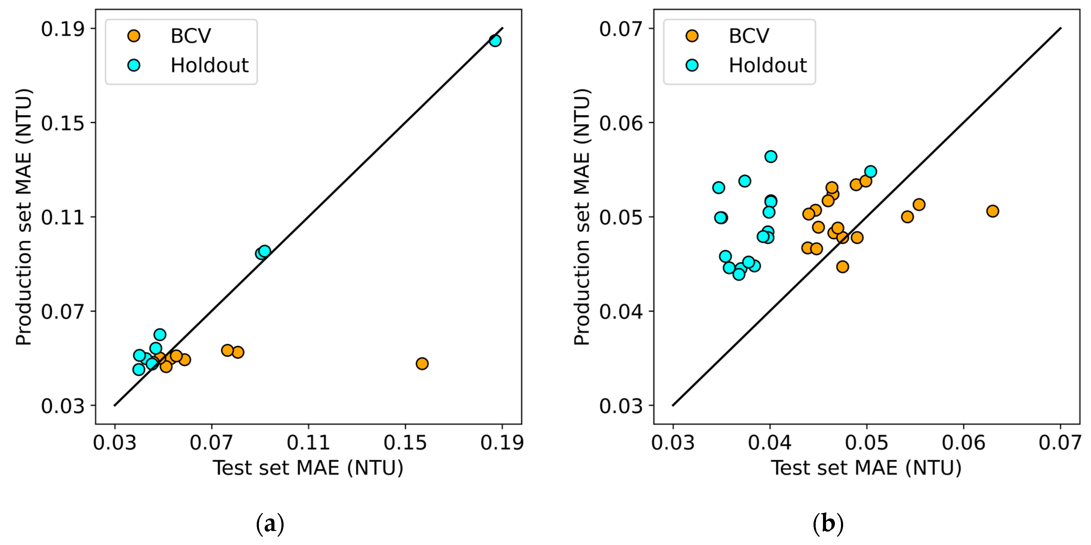
We re-evaluated all of our trained models using all the data from September 2020 to August 2021, representing one full year of operating data after the data used to train the model—we will refer to this particular subset of data as the production set. This effectively reflects the model’s performance if it were deployed to make real-time predictions in the industrial environment. Since this production set is now the same between the models trained using the two different methods, we can directly compare the two. In Figure 8 below, we plot the reported performance of each of the trained models on its test set against its performance on the production set. The diagonal line represents the line along which the reported test set error is the same as the observed error for the production set.

Figure 8.
Comparison of MAE on the test set and production set for: (a) multilayer perceptron models and (b) recurrent neural network models (both LSTM and GRU).
Figure 8a shows that all MLPs trained using BCV perform about the same on the production set despite the variability in their test set performance. In all nine cases, the models perform approximately as well or better on the production set than on the test set. Conversely, the production and test set performance for MLPs trained using holdout are very well correlated. A potential explanation is that the training set contains instances of extreme system behavior, such as notable flooding in the spring of 2019. In contrast, the production set is a relatively well-behaved year in this regard. It was observed through the training curves that the models trained using BCV with high test set error show particularly large errors where the test block contains this flood data, which raises the overall test error. This means that by the end of training using BCV, the reported test error may be skewed higher due to the test blocks containing extreme examples. The fact that the MLPs trained using BCV all perform similarly on the production set suggests that the use of BCV in this instance results in more stable models, as opposed to holdout which led several of the final models to perform poorly by comparison on this task.
In Figure 8b, all of the points representing RNNs trained using BCV are clustered relatively close to the line, which suggests that their test set performance is a good indicator of their production performance later on. On the other hand, it can be seen that all of the points representing RNNs trained using holdout lie above the line, indicating that their reported test set performance is an overestimate of their true performance in production. This is consistent with our earlier hypothesis that training using holdout would lead to underestimating the true model error for temporally dependent data. In this instance, RNNs trained using either method have similar production performance. The best model trained using BCV was the 3 × 64 GRU with a production set MAE of 0.045 NTU, and the best model trained using holdout was the 4 × 32 GRU with a very similar production set MAE of 0.044 NTU. However, as can be seen by the lower variability in the error of models trained using BCV, it seems to have an advantage over holdout in providing more robust estimates of model performance.
4. Discussion
4.1. Key Findings
We developed and tested three model types (MLP, LSTM, and GRU) using two training methodologies (blocked cross-validation and holdout) to predict clarified water turbidity in a conventional drinking water treatment plant. For each type of model, we trained a combination of different numbers and sizes of hidden layers and assessed each model on both a test set (which is different for BCV and holdout) and a production set (which was the same for both training methods).
When examining the best models of each type, MLP achieved similar MAE on the test set as both types of RNN (LSTM and GRU). In the case of training using BCV, the best examples of MLP, LSTM, and GRU had MAEs of 0.046, 0.046, and 0.044 NTU, whereas in the case of holdout training, these are 0.040, 0.035, and 0.035 NTU respectively. However, the obvious advantage of using either LSTM or GRU instead of MLP is that the range of performances varies widely for MLP depending on the model size, whereas for the RNNs, this variance is comparatively small. This is best appreciated visually in Figure 6 above. Of particular note is that the median error of the GRU models is only 0.001 and 0.002 NTU above the best model for BCV and holdout respectively. Therefore, GRU requires very little hyperparameter tuning to converge to a good model, as only trying a few different sizes is likely to uncover a model similar in performance to the best one found here. Conversely, the comparatively high variance in the performance of the MLP models implies that MLPs require much more hyperparameter tuning to find a good model. This somewhat nullifies MLP’s only advantage of being faster to train for smaller models, since it requires the training of a greater number of models in total.
Since the test set is different depending on whether we are training using blocked cross-validation or holdout due to the nature of these methods, we use the production data set to evaluate the models trained using either method to compare them. When comparing the two cross-validation methods, two different observations are made depending on the type of model being examined. In the case of MLP, we see that models trained using BCV result in similar production set MAE regardless of their wide range of test set MAE, whereas for models trained using holdout these two MAEs correlate quite well. In the case of RNNs, all models trained using holdout reported lower test MAE than production MAE, which is not the case for the RNNs trained using BCV where the production set MAE tends to be much closer to the test set MAE. This means that the RNNs trained using holdout consistently overestimated their performance during training and testing compared to how they would perform when deployed for real use.
Based on these results, we have demonstrated the advantages of using RNNs instead of MLPs and blocked cross-validation instead of holdout cross-validation for modelling time series problems in the water treatment sector. Therefore, we encourage any authors working on similar problems to adopt these methods as they require less hyperparameter tuning and better reflect real conditions, resulting in models with more reliable performance estimates. While these results are specific to this data set and this task and may not carry over to all similar tasks, the theory supports RNNs and blocked cross-validations being well suited to time series problems. We encourage authors to explore these avenues when modelling time series phenomena using machine learning.
4.2. Limitations and Future Work
While the results of this model are very good in that average prediction errors below 0.05 NTU are likely acceptable for use in a real water treatment plant, there is still further work that needs to be performed as part of integrating ML models into the water treatment process. Of great importance, this model was trained using historical data from a treatment plant that is overall well optimized and experiences very few process upsets. As we anticipate climate change to affect the quality of the source water over time, it is possible that future trends in this data will shift away significantly from those of the training set—this will likely degrade the model performance over time and we have no way of knowing in advance how robust our model predictions will be in the future as a result of changing climactic conditions. This highlights the importance of regularly re-training models as new data are generated over time, which is effectively a continuation of training with BCV with additional blocks available. There is also the issue that by their nature, extreme events will always make up only a small fraction of the training data set and therefore ML models which extract common patterns from significant amounts of historical data may not be the best way of predicting process performance in such cases.
Our model was developed to predict settled water turbidity based on what can be observed from historical data. While it was noted in the literature review that most authors developed models to predict optimal coagulant dose, we believe it is important to keep in mind that the applied coagulant dose that is observed in historical data is not necessarily optimal, since as we point out, we cannot optimize continuously based on the current standard of using jar tests for this purpose. Although the optimal coagulant dose would be a very useful variable to predict as it is most actionable for operators, such a model cannot be developed from historical data alone. With a model such as ours, we believe the utility comes from being able to alert operators when a large increase in settled water turbidity is expected and thus giving them advanced warning that a change to some process parameters may be required.
It is also important to note that our model is not causal—it merely makes predictions of future data based on previous data. It does not attempt to explain which changes in input result in corresponding changes in output. That is to say, it does not attempt to explain the underlying phenomenon. A potential future avenue to explore to address the above points is to generate data from a pilot-scale process to intentionally create scenarios of poor water quality and non-ideal process optimization to gather information on how this process performs under these rare circumstances. This approach allows us to gather data about extreme events much more quickly than if we waited for them to occur naturally. It allows us to experiment with different operational scenarios without risking distributed water quality, and to operate under the same conditions while following predictions from either jar tests or an ML model to see how these two methods compare. It also allows us to control each variable individually to examine how it affects the underlying process, gaining some insight into the causal relationships between the inputs and outputs of the coagulation process. This would allow for the development of models that can truly determine optimal coagulant dose since they would have access to training information that indicates how multiple different doses perform under the same raw water conditions. However, a potential drawback of this approach is that the model may not scale up correctly from the pilot-scale to the full-scale process. Thus, research investigating if models trained on pilot-scale data apply to full-scale processes would also be valuable.
Supplementary Materials
The following supporting information can be downloaded at: https://github.com/jakovaleks/RNN_BCV_DWT (accessed on 5 March 2024): all code developed for data management and analysis, model development and training, and creating figures for this paper.
Author Contributions
Conceptualization, A.J., L.C., and B.B.; Data curation, A.J.; Formal analysis, A.J.; Funding acquisition, B.B.; Investigation, A.J.; Methodology, A.J.; Project administration, B.B.; Resources, B.B.; Software, A.J.; Supervision, L.C. and B.B.; Validation, A.J., L.C. and B.B.; Visualization, A.J.; Writing—original draft, A.J.; Writing—review & editing, A.J., L.C. and B.B. All authors have read and agreed to the published version of the manuscript.
Funding
This research was funded by the Natural Sciences and Engineering Research Council of Canada Alliance grant program, grant number ALLRP 560764-20.
Data Availability Statement
Restrictions apply to the availability of these data. Data were obtained from Ville de Laval and are available from the authors with the permission of Ville de Laval. All of the code developed as part of this research can be found at: https://github.com/jakovaleks/RNN_BCV_DWT (accessed on 5 March 2024).
Acknowledgments
We would like to acknowledge the individual contributions of Martin Chrétien and Stamatios Tsoybariotis from Ville de Laval for gathering and providing us with the necessary data for this research.
Conflicts of Interest
The authors declare no conflict of interest. One of the funding sponsors (Ville de Laval) provided data for this research. One of the funding sponsors (Veolia) provided comments on the draft version of the paper.
References
- Desjardins, C.; Koudjonou, B.; Desjardins, R. Laboratory study of ballasted flocculation. Water Res. 2002, 36, 744–754. [Google Scholar] [CrossRef]
- Ratnaweera, H.; Fettig, J. State of the Art of Online Monitoring and Control of the Coagulation Process. Water 2015, 7, 6574–6597. [Google Scholar] [CrossRef]
- Van Benschoten, J.E.; Jensen, J.N.; Rahman, M.A. Effects of Temperature and pH on Residual Aluminum in Alkaline-Treated Waters. J. Environ. Eng. 1994, 120, 543–559. [Google Scholar] [CrossRef]
- ASTM International. ASTM International. ASTM D2035-19: Standard Practice for Coagulation-Flocculation Jar Test of Water. In Book of Standards; ASTM International: West Conshohocken, PA, USA, 2019; Volume 11.02. [Google Scholar]
- Adgar, A.; Cox, C.S.; Jones, C.A. Enhancement of coagulation control using the streaming current detector. Bioprocess Biosyst. Eng. 2005, 27, 349–357. [Google Scholar] [CrossRef] [PubMed]
- Sibiya, S.M. Evaluation of the Streaming Current Detector (SCD) for Coagulation Control. Procedia Eng. 2014, 70, 1211–1220. [Google Scholar] [CrossRef]
- Edzwald, J.; Kaminski, G.S. A practical method for water plants to select coagulant dosing. J. New Engl. Water Work. Assoc. 2009, 123, 15–31. [Google Scholar]
- Jackson, P.J.; Tomlinson, E.J. Automatic Coagulation Control–Evaluation of Strategies and Techniques. Water Supply 1986, 4, 55–67. [Google Scholar]
- Robinson, W.A. Climate change and extreme weather: A review focusing on the continental United States. J. Air Waste Manag. Assoc. 2021, 71, 1186–1209. [Google Scholar] [CrossRef]
- Bladon, K.D.; Emelko, M.B.; Silins, U.; Stone, M. Wildfire and the future of water supply. Environ. Sci. Technol. 2014, 48, 8936–8943. [Google Scholar] [CrossRef]
- Slavik, I.; Uhl, W. A new data analysis approach to address climate change challenges in drinking water supply. In Proceedings of the IWA DIGITAL World Water Congress, Copenhagen, Denmark, 24 May – 4 June 2021. [Google Scholar]
- Gómez-Martínez, G.; Galiano, L.; Rubio, T.; Prado-López, C.; Redolat, D.; Paradinas Blázquez, C.; Gaitán, E.; Pedro-Monzonís, M.; Ferriz-Sánchez, S.; Añó Soto, M.; et al. Effects of Climate Change on Water Quality in the Jucar River Basin (Spain). Water 2021, 13, 2424. [Google Scholar] [CrossRef]
- Lee, J.M.; Ahn, J.; Kim, Y.D.; Kang, B. Effect of climate change on long-term river geometric variation in Andong Dam watershed, Korea. J. Water Clim. Chang. 2021, 12, 741–758. [Google Scholar] [CrossRef]
- Baxter, C.W.; Stanley, S.J.; Zhang, Q.; Smith, D.W. Developing artificial neural network models of water treatment processes: A guide for utilities. J. Environ. Eng. Sci. 2002, 1, 201–211. [Google Scholar] [CrossRef]
- Griffiths, K.A.; Andrews, R.C. The application of artificial neural networks for the optimization of coagulant dosage. Water Supply 2011, 11, 605–611. [Google Scholar] [CrossRef]
- Santos, F.C.R.d.; Librantz, A.F.H.; Dias, C.G.; Rodrigues, S.G. Intelligent system for improving dosage control. Acta Sci. Technol. 2017, 39, 33. [Google Scholar] [CrossRef]
- Jayaweera, C.D.; Aziz, N. Development and comparison of Extreme Learning machine and multi-layer perceptron neural network models for predicting optimum coagulant dosage for water treatment. J. Phys. Conf. Ser. 2018, 1123, 012032. [Google Scholar] [CrossRef]
- Fan, K.; Xu, Y. Intelligent control system for flocculation of water supply. J. Phys. Conf. Ser. 2021, 1939, 012064. [Google Scholar] [CrossRef]
- Goodfellow, I.; Bengio, Y.; Courville, A. Deep Learning; The MIT Press: Cambridge, MA, USA, 2016. [Google Scholar]
- Kaufman, S.; Rosset, S.; Perlich, C.; Stitelman, O. Leakage in data mining. ACM Trans. Knowl. Discov. Data 2012, 6, 1–21. [Google Scholar] [CrossRef]
- Snijders, T.A.B. On Cross-Validation for Predictor Evaluation in Time Series. In Proceedings of the On Model Uncertainty and its Statistical Implications, Groningen, The Netherlands, 25–26 September 1986; pp. 56–69. [Google Scholar]
- Bergmeir, C.; Benítez, J.M. On the use of cross-validation for time series predictor evaluation. Inf. Sci. 2012, 191, 192–213. [Google Scholar] [CrossRef]
- Meteorological Service of Canada. Canadian Climate Normals 1981–2010 Station Data: Montreal/Pierre Elliott Trudeau Intl A; Meteorological Service of Canada: Dorval, QC, Canada, 2023. [Google Scholar]
- Veolia Water Technologies. ACTIFLO® HCS. Available online: https://www.veoliawatertechnologies.com/en/solutions/technologies/actiflo-hcs (accessed on 16 May 2023).
- Ministère de l’Environnement de la Lutte Contre les Changements Climatiques de la Faune et des Parcs. Banque de Données sur la Qualité du Milieu Aquatique. 2002. Available online: https://www.environnement.gouv.qc.ca/eau/atlas/documents/conv/ZGIESL/2002/Haut-St-Laurent_et_Grand_Montreal_2000-2002.xlsx (accessed on 26 March 2024).
- Hochreiter, S.; Schmidhuber, J. Long Short-Term Memory. Neural Comput. 1997, 9, 1735–1780. [Google Scholar] [CrossRef]
- Cho, K.; Van Merrienboer, B.; Gulcehre, C.; Bahdanau, D.; Bougares, F.; Schwenk, H.; Bengio, Y. Learning Phrase Representations using RNN Encoder-Decoder for Statistical Machine Translation. arXiv 2014, arXiv:1406.1078. [Google Scholar] [CrossRef]
- Chung, J.; Gulcehre, C.; Cho, K.; Bengio, Y. Empirical Evaluation of Gated Recurrent Neural Networks on Sequence Modeling. In Proceedings of the NIPS 2014 Deep Learning and Representation Learning Workshop, Montreal, Quebec, Canada, 12–13 December 2014. arXiv 2014, arXiv:1412:3555. [Google Scholar] [CrossRef]
- Williams, R.J.; Zipser, D. A Learning Algorithm for Continually Running Fully Recurrent Neural Networks. Neural Comput. 1989, 1, 270–280. [Google Scholar] [CrossRef]
- Arlot, S.; Celisse, A. A survey of cross-validation procedures for model selection. Stat. Surv. 2010, 4, 40–79. [Google Scholar] [CrossRef]
- Zhang, K.; Achari, G.; Li, H.; Zargar, A.; Sadiq, R. Machine learning approaches to predict coagulant dosage in water treatment plants. Int. J. Syst. Assur. Eng. Manag. 2013, 4, 205–214. [Google Scholar] [CrossRef]
- Godo-Pla, L.; Emiliano, P.; Valero, F.; Poch, M.; Sin, G.; Monclús, H. Predicting the oxidant demand in full-scale drinking water treatment using an artificial neural network: Uncertainty and sensitivity analysis. Process Saf. Environ. Prot. 2019, 125, 317–327. [Google Scholar] [CrossRef]
- Wang, D.; Wu, J.; Deng, L.; Li, Z.; Wang, Y. A real-time optimization control method for coagulation process during drinking water treatment. Nonlinear Dyn. 2021, 105, 3271–3283. [Google Scholar] [CrossRef]
- Kingma, D.P.; Ba, J. Adam: A Method for Stochastic Optimization. In Proceedings of the 3rd International Conference for Learning Representations, San Diego, CA, USA, 7–9 May 2015. [Google Scholar]
Disclaimer/Publisher’s Note: The statements, opinions and data contained in all publications are solely those of the individual author(s) and contributor(s) and not of MDPI and/or the editor(s). MDPI and/or the editor(s) disclaim responsibility for any injury to people or property resulting from any ideas, methods, instructions or products referred to in the content. |
© 2024 by the authors. Licensee MDPI, Basel, Switzerland. This article is an open access article distributed under the terms and conditions of the Creative Commons Attribution (CC BY) license (https://creativecommons.org/licenses/by/4.0/).