A Boatable Days Framework for Quantifying Whitewater Recreation—Insights from Three Appalachian Whitewater Rivers

Abstract

Outdoor recreation is one of the fastest-growing economic sectors in the United States and is being used by communities to support economic development, social prosperity, and environmental protection. For communities that have whitewater rivers, whitewater recreation provides a powerful economic alternative to ailing extractive and manufacturing industries that have long dominated rural communities. In order to promulgate a whitewater recreation-based economy, stakeholders need information about their whitewater resources, including how often and when they can be paddled. The overall goal of this study, therefore, was to develop an analytical framework that quantifies boatable days, that is, the number of days that streamflow exceeds the minimum boatable flow levels needed to paddle downstream. Importantly, our framework uses publicly available streamflow and minimum boatable flow information that can be used to quantify boatable days for any whitewater run in the country, irrespective of watershed size or river flashiness. We applied the framework to three world-class whitewater rivers in the central Appalachian Mountains, USA, and found abundant and stable boating opportunities throughout the year. Our results underscore the potential for strategically developing whitewater recreation as a means of economic diversification and highlight how boatable days analysis can be used for quantifying whitewater resources.

1. Introduction

Outdoor recreation is a significant and growing economic sector in the United States. In 2022, outdoor recreation generated USD 1.1 trillion in economic output and contributed USD 564 billion of value-added dollars, accounting for 2.2% of the US Gross Domestic Product (GDP) [1]. As a result, communities throughout the country are leveraging outdoor recreation assets to support economic development, community health, social prosperity, and environmental protection, colloquially referred to as the “outdoor economy” [2]. As the outdoor economy continues to evolve, greater emphasis is being placed on its potential for promoting positive social, health, education, and economic outcomes [3]. With the passage of the Outdoor Recreation Jobs and Economic Impact Act of 2016, which directs the Department of Commerce to assess and analyze the outdoor recreation economy in the United States [4,5], and, more recently, the passage of the Great American Outdoors Act of 2020, which, among other things, fully funds the Land and Water Conservation Fund, the federal government is signaling the role of the outdoor economy for helping to revitalize ailing communities left behind from deindustrialization and the transition from fossil fuel extraction economies [6]. Promulgating the outdoor economy, however, requires information, data, and tools that can be used by communities, businesses, planners, and decision makers to assess local recreational assets.

For communities that have whitewater rivers, whitewater recreation offers unique and geographically constrained economic development opportunities as alternatives to ailing extractive and manufacturing industries that have long dominated rural mountain communities. Whitewater recreation, which includes kayaking, canoeing, and rafting on whitewater rivers, benefits communities in several ways. It supports local economies through tourism, commercial rafting, and guide businesses; outdoor equipment innovation, manufacturing, and retail; and generates jobs, taxes, and amenities. Furthermore, whitewater rivers provide environmental aesthetics, healthy living, and unique amenities for attracting new residents. In 2017, Americans spent nearly USD 140 million on water sports recreation, directly supporting 1.2 million jobs that generated USD 43.9 million in salaries and wages, USD 10.6 billion in federal taxes, and USD 9.6 billion in state and local taxes [7]. At the local scale, the economic impact of whitewater recreation is evident. On the world-famous Gauley River in West Virginia, commercial and non-commercial recreation generated USD 4.68 million [8]. On the Cheoah River in Tennessee, sixteen scheduled whitewater releases generate USD 3 million annually [9]. In western North Carolina, commercial and non-commercial paddlers traveling to the Nantahala and Pisgah National forests generated over USD 39 million in revenue [10], while paddlers traveling to three national forests in Colorado spent USD 4.7 million, generating USD 538,000 in job income [11].

A defining feature of whitewater rivers are rapids that are created when streamflow, gradient, constrictions, and obstructions interact to create a myriad of challenges and risks that motivate the whitewater paddler. Given the combination of these geographic factors, whitewater rivers are concentrated around mountains that have more precipitation, runoff, and topographic gradient (e.g., Viviroli et al. [12]) than lower-lying areas. Streamflow, the volume of water flowing in a stream or river per time (e.g., cubic meters per second), exerts a first-order control on whitewater recreation. Without sufficient streamflow, a whitewater run (a specific stretch of a whitewater river or creek) may not be physically, realistically, or enjoyably paddled (see Rood et al. [13], Zinke et al. [14]). Given the dependence of whitewater paddling on streamflow levels, a handful of studies have combined streamflow data with minimum boatable flow levels to calculate two key metrics that can be used to describe whitewater recreational assets—how often and when a given whitewater run can be paddled. Threshold-based approaches (e.g., [15]), which are used to truncate streamflow data above and below the defined threshold, are widely used in hydrology to study drought [16], runoff generation [17,18], hydrologic modeling and forecasting [19], and recreational and environmental flow [13,20]. Mayfield [9] calculated boatable days, the number of days a year that streamflow exceeded the minimum flow thresholds, for three whitewater runs in the southern Appalachian Mountains, USA. Using mean daily streamflow from three United States Geological Survey gaging stations and published minimum boatable flow levels, [9] found that whitewater runs on the Obed–Emory, Nolichucky, and Watauga rivers could be boated 99 days/year (27% of days in a year), 304 days/year (83%), and 89 days/year (24%), respectively. Using simulated streamflow from simple rainfall-runoff models and published minimum flow thresholds, Ligare et al. [21] quantified boating on 128 runs in the Sierra Nevada Mountains in California. Originally reported as boatable weeks (and converted to boatable days for the current paper), boatable days ranged from a handful of days/year to more than 100 days/year. Stafford et al. [22] combined mean daily streamflow data with user experience surveys to quantify commercial and non-commercial boatable days on the Cataract Canyon section of the Colorado River and found that it was boatable 257 to 365 days/year. And Bowman et al. [23] combined expert knowledge of minimum and maximum flow conditions with daily streamflow data to find that the Collingwood River in Tasmania, Australia, could be boated, on average, 321 days/year.

While insightful, the use of mean daily and weekly streamflow in the aforementioned studies could be problematic for quantifying boatable days for whitewater runs situated on small rivers and creeks that respond quickly to rainfall. For these types of runs, the window of favorable boating conditions is likely shorter, e.g., on the order of a few hours or less. For these cases, the use of mean daily streamflow (or coarser) could result in the underestimation of boating days. Large rivers, on the other hand, like many of those analyzed in the previous studies, have large contributing drainage areas and more groundwater that sustain streamflow over longer periods of time (e.g., Gianfagna et al. [24]). Mean daily streamflow likely captures the temporal dynamics of whitewater runs on larger river systems. Furthermore, the dependence of boating on streamflow makes whitewater recreation and its economy potentially vulnerable to climate change [25,26,27]. With warming air temperatures, some regions of the United States are becoming drier (e.g., intermountain west), other areas (e.g., northeast) are becoming wetter, and heavy rainfall is increasing throughout the country [28]. Climate change has important implications for watersheds, ecosystems, and the communities that depend on them for economic development. Understanding the stability of whitewater boating opportunities over the recent past can provide important insights for developing and promulgating sustainable outdoor recreation economies into the 21st century.

Rectifying the potential mismatch between favorable boating conditions and the timescales of boatable days analysis is particularly important for assessing whitewater resources in mountainous environments dominated by small headwater creeks and rivers. A case in point is the central Appalachian Mountains region in the eastern USA, which includes West Virginia, southwestern Pennsylvania, and western Maryland. With vast forests, steep, heavily dissected headwater watersheds, and an abundance of streams, creeks, and rivers, the region has a high concentration of whitewater. With whitewater runs on rivers that include the Cheat, New, Gauley, and Youghiogheny rivers, the region is known globally for world-class whitewater. Furthermore, the region is within a day’s drive of sixty percent of the country’s population [29] and a few hours from major metropolitan centers that include Washington, DC, Pittsburgh, and Columbus, Ohio. Like many rural places, the region is undergoing a rapid economic transition away from coal and toward outdoor recreation and other forms of sustainable economic development (e.g., wind and solar) [30,31]. In 2023, for example, the economic impact of tourism in West Virginia alone exceeded USD 7 billion, which represents a 17% increase in visitor spending compared to prior 2020 [32]. Strategically developing and promulgating a whitewater economy here and in other places dominated by creeks and small rivers requires a more flexible approach that can accurately capture boating opportunities at sub-daily timescales.

In response to this need, we developed a framework that can quantify boatable days for any whitewater section in the country, irrespective of watershed size and streamflow flashiness, so far as streamflow and minimum boatable flow threshold information is available. We applied the framework to three world-renowned whitewater runs—the Upper Blackwater and Lower Big Sandy located in West Virginia and the Upper Youghiogheny located in western Maryland (Figure 1). The overall goal of this study was to quantify boatable days across timescales (e.g., monthly, seasonal, annual) and evaluate the sensitivity of boatable days across time. Importantly, we demonstrate for the first time how instantaneous maximum streamflow can be used to estimate boatable days for flashier whitewater runs, thereby filling critical knowledge and methodological gaps that are crucial for developing and promulgating whitewater economies throughout the US.

To meet this study’s goals, we (1) developed a boatable days framework in the open source statistical software R Studio (v. 2023.12.1) that downloads, analyzes, and aggregates streamflow time-series data from USGS gaging stations; (2) calculated boatable days at monthly, seasonal, and annual timescales using mean daily and instantaneous maximum streamflow; and (3) evaluated for changes in boatable days at the different timescales using trend analysis. Furthermore, we discuss the seasonal hydrology that generates boatable flows to provide insight for other whitewater runs in the region and discuss tradeoffs of instantaneous maximum and mean daily streamflow for quantifying boatable days.

2. Materials and Methods

2.1. Study Location

The three whitewater runs evaluated in this study are located in the highlands region of the central Appalachian Mountains (Figure 1). This heavily forested, mountainous region has a vast network of streams, creeks, and rivers that provide freshwater services to communities, economies, and ecosystems in the eastern and midwestern US. West Virginia alone boasts 86,000 km of rivers that serve as the headwaters to the Potomac River that drains east to the Chesapeake Bay, and the Ohio River, the largest and most biologically diverse tributary of the Mississippi River [33,34]. Two of the runs, the Upper Blackwater and the Lower Big Sandy, are headwater tributaries to the Cheat River in northeastern West Virginia. The Upper Youghiogheny (herein referred to as the Upper Yough) is located in the Youghiogheny River watershed in western Maryland. Both watersheds are tributaries of the Monongahela River, which confluences with the Allegheny River to form the Ohio River that drains to the Mississippi River and the Gulf of Mexico.

The climate of the region is cool, humid, and continental [35]. Long-term, thirty-year (1980–2020) normal air temperature averaged 9.3 °C across the three watersheds (

Table 1. Watershed, climate, streamflow, and minimum boatable flow threshold characteristics for the three whitewater runs examined in this study: the Upper Blackwater, Lower Big Sandy, and Upper Youghiogheny rivers.

Whitewater Section	USGS Stream Station	Latitude/Longitude	Gauge Elevation	Watershed Drainage Area	Mean Annual Air Temperature	Mean Annual Precipitation	Min. Annual Streamflow	Mean Annual Streamflow	Max. Annual Streamflow	Minimum Boatable Threshold
			m	km2	deg. C	mm	m3/s	m3/s	m3/s	m3/s
Upper Blackwater	3066000	39°07′37″/79°28′07″	932	223	9.3	1323	2.17	223	4000	7.08
Lower Big Sandy	3070500	39°37′18″/79°42′16″	403	518	10.4	1188	2.82	436	10,500	7.28
Upper Yough	3076500	39°39′13″/79°24′29″	453	764	9.3	1167	38.5	699	9560	12.74

), while monthly temperature ranged from −3.0 °C in January to 21.7 °C in July [36]. Long-term, thirty-year (1980–2020) normal precipitation, mostly in the form of rainfall, is relatively evenly distributed throughout the year, averaging 1226 mm across the three watersheds. Precipitation during late summer and early fall can be intense due to localized convective warming and tropical storms from the Gulf of Mexico and Atlantic Ocean [34,37]; historical 24 h rainfall frequently exceeds 100 mm [38]. Frontal storms in winter bring cold temperatures and frequent rain and snowfall that form transient snowpack and snowmelt-fed runoff [39]. Streamflow is dominated by base flow while stormflow is dominated by rainfall [40]. Soils are shallow and underlain by relatively impermeable sedimentary rocks with limited soil water storage. As a result, streamflow is characterized as flashy, rapidly responding to precipitation, especially in small rivers and headwater catchments [34]. The mixed deciduous forests that cover the region exert strong seasonal influences on runoff and streamflow. During the forest growing season, which spans from May to October [40], antecedent moisture is low and stream base flow is suppressed due to high forest evapotranspiration. Hence, more precipitation is necessary to generate streamflow during the growing season. During the leaf-off dormant season, forest evapotranspiration is suppressed, and antecedent moisture and base flow are elevated. During the dormant season, it takes less precipitation to generate runoff and streamflow.

The three whitewater runs considered in this study are representative of whitewater rivers throughout the region. The Upper Blackwater is a steep, rain-fed section of the Blackwater River watershed, which drains 368 km² of high-elevation forests and wetlands located on the Canaan Valley National Wildlife Refuge. From 2000–2020, minimum, mean, and maximum daily streamflow measured at the USGS Blackwater River at Davis, WV (03066000) gauge were 2.17 m³/s, 223 m³/s, and 4000 m³/s (Table 1). With a maximum gradient of nearly 61 m/km over the 3.8 km run, the Upper Blackwater offers some of the best technical expert wilderness boating in the eastern United States [41]. The Lower Big Sandy is a high-volume, rain-fed section of the Big Sandy Creek that drains mixed land cover dominated by forests, agriculture, and several small communities. The minimum, mean, and maximum daily streamflow measured at the USGS Big Sandy Creek at Rockville, WV (03070500) gauge were 2.82 m³/s, 436 m³/s, and 10,500 m³/s. With 8 km of technically expert whitewater including two waterfalls (5 m and 4 m) and a maximum gradient of 24 m/km, the Lower Big Sandy is “one of the finest stretches of whitewater on the continent” [41]. The Upper Yough is a rain-fed and seasonally dam-controlled section of the Youghiogheny River, which is also dominated by forests, agriculture, and several small communities. The minimum, mean, and maximum daily streamflow measured at the USGS Youghiogheny River at Friendsville, Maryland (03076500) gauge were 38.5 m³/s, 699 m³/s, and 9560 m³/s. The 15 km section of technical whitewater is “one of the most legendary stretches of whitewater on the continent” [41]. With a maximum gradient of 29 m/km, it has long served as a training ground for technical whitewater boaters in the east. While scheduled whitewater releases from the Deep Creek Lake hydroelectric dam provide boatable flows from April to mid-October, the Upper Yough also runs on natural rainfed and snowmelt flows from the unregulated, 4.5 km “Top Yough”, another technical whitewater run.

2.2. Workflow, Data and Analysis

An overarching goal of this study was to provide a flexible framework that can be used by stakeholders to quantify boatable days for any whitewater run in the US. As such, our analysis was based on two publicly available datasets that have consistent national coverage: the American Whitewater (AW) National Whitewater Inventory (NWI) and the United States Geological Survey (USGS) stream gaging network. The NWI is the principal source of information for whitewater runs in the United States and several international locations. The NWI includes information on river and whitewater run name; difficulty, length, and gradient; streamflow gauge information, real-time streamflow conditions, and recommended minimum and maximum streamflow levels; geographic coordinates; and a dynamic map of put-in and take-out locations as well as photographs, news, advocacy issues, and accidents (https://www.americanwhitewater.org/content/River/view/river-index accessed on 15 September 2022). While first descents of new or obscure whitewater runs may not be included in the database, the NWI is the authoritative and go-to dataset for paddlers, commercial operators, and managers (e.g., Federal Energy Regulatory Commission).

To a certain extent, minimum boatable flow levels are subjective [9]. Beyond having enough water to physically paddle downstream, the choice to paddle a run at a given “minimum” flow level ultimately depends on the type of craft and skill of the boater; skilled kayakers and canoers can navigate water levels substantially lower than rafters. Notwithstanding, minimum boatable flow levels are largely developed through community consensus [9] and published in guidebooks and websites (e.g., https://www.americanwhitewater.org/, accessed on 15 September 2022). Maximum boatable flow levels are more individual; skilled whitewater boaters regularly paddle whitewater runs at flows larger than the recommended cutoff levels [9]. For this reason, the boatable days analysis in our study was restricted to minimum levels. According to the NWI, the minimum flow for the Upper Blackwater was 7.1 m³/s measured at the USGS Blackwater River at Davis, WV (03066000) gauge (Table 1). Minimum thresholds for both the Lower Big Sandy and Upper Yough were reported as stages. To standardize analysis, we converted minimum stage levels to volumetric streamflow using published USGS stage-streamflow rating curves for each gauge. The minimum boatable flow for the Lower Big Sandy was 7.3 m³/s measured at the USGS Big Sandy Creek at Rockville, WV (03070500) gauge and 12.7 m³/s for the Upper Yough measured at the USGS Youghiogheny River at Friendsville, Maryland (03076500) gauge.

The workflow for the boatable days’ analyses is summarized in Figure 2. Briefly, boatable days were calculated in the R programming environment [42] using the two different streamflow datasets for a twenty-year study period from 1 January 2000 to 31 December 2020. The first approach, following Mayfield, 2006, used mean daily streamflow (Qmean), defined as the average streamflow over a 24 h period. A primary benefit of using Qmean is that it is published as a complete dataset, i.e., the USGS interpolates missing data. Daily Qmean data for the three runs were extracted from the USGS National Water Information System (NWIS) using the USGS eight-digit station number and the R package dataRetrieval [43]. dataRetrieval simplifies working with USGS water data by dynamically finding and downloading data directly into the R. Once in the R environment, streamflow for each day was screened using the ‘mutate’ and ‘summarise_all’ functions in the dplyr [44] package to determine if it exceeded the minimum boatable flow. When Qmean exceeded the minimum flow threshold, the day was determined to be boatable. Boatable days were then summarized by month, season, and year.

The second approach used instantaneous maximum streamflow (Qinst), defined as the highest instantaneous streamflow measurement during a 24 h period. The complexity of using Qinst data was significantly greater than using Qmean data for three reasons. One, Qinst data were not available through dataRetrieval, so data for each station were manually downloaded from the NWIS Web Interface (https://waterdata.usgs.gov/nwis accessed 15 January 2022), saved as *.csv files, and manually loaded into R (Figure 2). Two, Qinst data are recorded and published at the raw timestep of measurement, which varies across stations and time periods. For the stations analyzed in this study, measurements were recorded at 15, 30, and 60 min intervals that varied over time and included multiple measurements for each day. Measurement intervals for the Big Sandy Creek at Rockville, WV station, for example, were recorded in 60 min intervals from January 2001 to mid-October 2008; then, 30 min intervals until September 2011, and, finally, 15 min intervals for the remainder of the study period. This amounted to 427,386 Qinst measurements over the twenty-year study compared to 7304 Qmean measurements. Three, unlike Qmean, the Qinst datasets contained missing data across different measurement intervals, resulting in a fragment, non-continuous dataset with different intervals. For the Big Sandy station, this amounted to 828 days (11%) days over the twenty-year study that contained missing data .

R code was developed to address these challenges, simplify the analysis, and provide a more user-friendly workflow for future applications by interested users. Briefly, after manually importing the Qinst dataset, a continuous hourly time-series dataset was constructed using the padr (https://github.com/EdwinTh/padr, accessed 20 April 2024) package. Then, the largest Qinst measurement within a 60 min period was assigned to each hour using dplyr [44]. And, finally, similar to the Qmean analysis, boatable days were calculated for month, season, and year using the ‘mutate’ and ‘summarise_all’ functions part of the dplyr [44]. Data generated in each step of the Qinst analysis were automatically exported and written to a *.csv file for quality control and future analysis.

The nonparametric Mann–Kendall (MK) trend test, a rank-based approach commonly used in hydrology and climatological studies [18,45], was used to assess the stability of boatable days over time at annual and monthly timescales. An important requirement of MK is serial independence [46], which was tested using the Ljung–Box Test [47]. Serial correlation was not detected in either the annual or monthly data. For the annual data, MK was applied to the continuous time series of annual boatable days. For the monthly data, MK was applied to time series structured by month and year, i.e., boatable days January 2000, January 2001, …, January 2020. Mann–Kendall was implemented in R using the trend package [48]. The slope of each trend was calculated as the median of all possible pair-wise slopes, commonly referred to as the Sen slope [46,49]. Statistically significant trends were assessed using α = 0.05.

3. Results

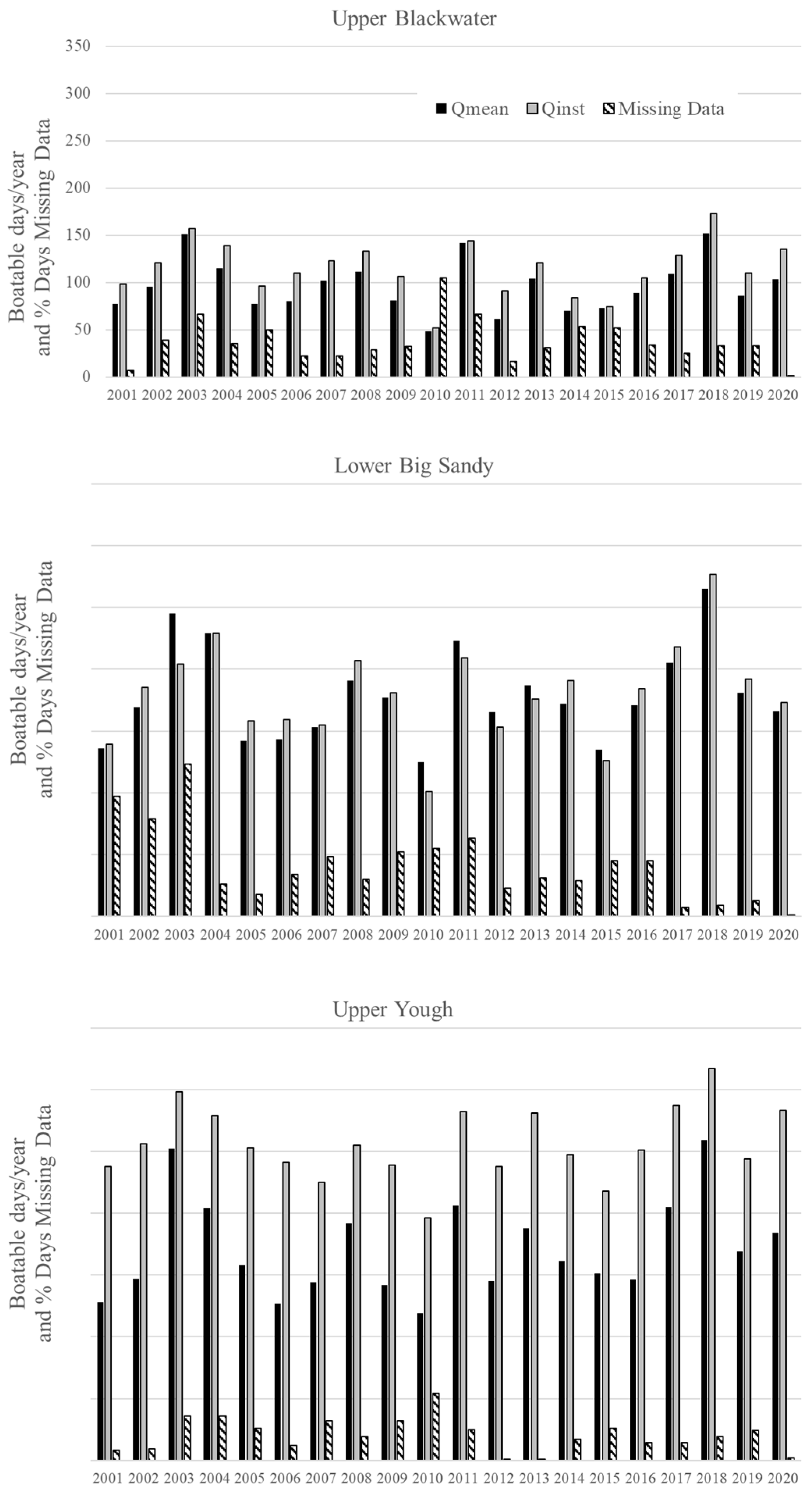
3.1. Annual Boatable Days

The number of boatable days/year from 2001 to 2020 is summarized in Table 3 and shown in Figure 3. Boatable days for the Upper Blackwater averaged 100 days/year (standard deviation = ±28 days/year) based on Qmean and 116 days/year (±28 days/year) based on Qinst. For the Lower Big Sandy, boatable days averaged 179 (±37) days/year and 180 (±38) days/year for Qmean and Qinst, respectively. Boatable days for Upper Yough averaged 171 (±38) days/year for Qmean and 256 (±29) days/year for Qinst. While there were no missing data in the Qmean datasets, 751 days or 10% of days were missing from the Qinst dataset for the Upper Blackwater, 828 days (11%) for the Lower Big Sandy, and 417 days (6%) for the Upper Yough (

Table 2. Annual boatable days from 2001 to 2020 for the Upper Blackwater, Lower Big Sandy, and Upper Yough whitewater sections using mean daily streamflow (Qmean) and instantaneous maximum streamflow (Qinst) for the three respective USGS stations.

Section	Time Period	Qmean		Qinst
		Number of Boatable Days	Number of Days Missing Q	Number of Boatable Days	Number of Days Missing Q
		Days (%)	Days	Days (%)	Days (%)
Upper Blackwater	2001–2020	100 (27%)	0	116 (32%)	751 (10%)
Lower Big Sandy	2001–2020	179 (49%)	0	180 (49%)	828 (11%)
Upper Yough	2001–2020	171 (47%)	0	256 (67%)	417 (6%)

).

According to the Mann–Kendall trend analysis, annual boatable days did not significantly change over the study period (α = 0.05) (

Table 3. Trend analysis and changes in annual boatable days from 2000 to 2021 for the Upper Blackwater, Lower Big Sandy, and Upper Yough whitewater sections based on the Mann–Kendall trend test at α = 0.05 for mean daily streamflow (Qmean) and instantaneous maximum streamflow (Qinst). Total change (D) was calculated as Sen slope coefficient times the number of years in the study period, 20 years.

Section	Qmean			Qinst
	p-Value	Slope	Total D	p-Value	Slope	Total D
	-	Days/yr	Days	-	Days/yr	Days
Upper Blackwater	0.70	0.41	8	0.57	-0.74	-15
Lower Big Sandy	0.54	1.50	30	0.2	1.5	30
Upper Yough	0.26	1.57	31	1.00	-0.08	-2

). Notwithstanding, Sen slopes were positive across all runs based on Qmean. Sen slope was also positive for the Lower Big Sandy using Qinst but was negative for the Upper Blackwater and Upper Yough.

3.2. Monthly Boatable Days

The number of boatable days by month and by season are shown in Figure 4 and summarized in

Table 4. Mean monthly and seasonal boatable days from 2001 to 2020 for the Upper Blackwater, Lower Big Sandy, and Upper Youghiogheny whitewater sections using mean daily streamflow (Qmean) and instantaneous maximum streamflow (Qinst) for respective USGS stations.

Month	Season	No. of Days	Upper Blackwater				Lower Big Sandy				Upper Yough
			Qmean Boat. Days	Qinst Boat. Days	Missing Days	% Missing Days	Qmean Boat. Days	Qinst Boat. Days	Missing Days	% Missing Days	Qmean Boat. Days	Qinst Boat. Days	Missing Days	% Missing Days
Dec	Winter	620	11	13	127	20	22	22	52	8	21	24	55	9
Jan		621	11	12	277	45	21	20	188	30	21	19	163	26
Feb		565	12	12	187	33	22	19	154	27	24	20	133	24
Mar		620	15	16	55	9	26	25	50	8	21	25	20	3
Apr	Spring	600	14	16	1	0.2	24	25	5	1	19	24	16	3
May		620	11	13	4	1	21	22	7	1	9	24	0	0
Jun		600	5	7	6	1	9	10	54	9	7	22	1	0
Jul	Summer	620	4	6	9	1	6	8	49	8	4	26	0	0
Aug		620	2	3	14	2	4	6	102	16	4	22	1	0
Sep		600	3	3	19	3	3	4	68	11	7	17	2	0
Oct	Fall	620	4	5	15	2	7	8	67	11	12	15	6	1
Nov		600	6	8	29	5	13	13	32	5	21	17	20	3
	Average		8	10	-	-	15	15	-	-	14	21	-	-

. Monthly boatable days for the Upper Blackwater averaged 8 days/month, ranging from 2 days in August to 15 days in March for Qmean. For Qinst, boatable days averaged 10 days/month, ranging from 3 days in August and September to 16 days in March and April. For the Lower Big Sandy, boatable days averaged 15 days/month and ranged from 3 days in September to 26 days in March based on Qmean. Using Qinst, boatable days averaged 15 days/month and ranged from 4 days in September to 25 days in both March and April. Monthly boatable days for the Upper Yough averaged 14 days/month and ranged from 4 days in August to 24 days in February based on Qmean. For Qinst, boatable days averaged 21 days/month and ranged from 15 days in October to 26 days in July.

Boatable days were distinctly seasonal (Figure 4) with the greatest number of days generally occurring during spring (March, April, May), followed by winter (Decemeber, January, February), fall (September, October, November), and then summer (June, July, August) for the Upper Blackwater and Lower Big Sandy. In the Upper Yough, boatable days were more variable based on the approach used. Using Qmean, the greatest number of boatable days occurred during the winter with 22 days, closely followed by fall (21 days), spring (17 days), and then summer (5 days). Using Qinst, however, spring has the greatest number of days (25), followed by summer (23 days), then winter (21 days), and, finally, fall (16 days).

Again, the Qmean datasets did not contain any missing data but missing days were present throughout the monthly Qinst datasets (

Table 5. Trend analysis and changes in monthly boatable days from 2000 to 2021 in the Upper Blackwater, Lower Big Sandy, and Upper Yough whitewater sections based on the Mann–Kendall trend test for mean daily streamflow (Qmean) and instantaneous maximum streamflow (Qinst). Total D calculated as Sen slope coefficient x number of years. Bolded values show statistical significance at α = 0.05.

Month	Season	Upper Blackwater						Lower Big Sandy						Upper Yough
		Qmean			Qinst			Qmean			Qinst			Qmean			Qinst
		p-Value	Slope	Total D	p-Value	Slope	Total D	p-Value	Slope	Total D	p-Value	Slope	Total D	p-Value	Slope	Total D	p-Value	Slope	Total D
		-	Days/Year	Days	-	Days/Year	Days	-	Days/Year	Days	-	Days/Year	Days	-	Days/Year	Days	-	Days/Year	Days
Dec	winter	0.14	0.35	7	0.25	0.19	4	0.92	0.00	0	0.77	−0.09	−2	0.62	0.1	2	0.27	0.3	5
Jan		0.36	0.14	3	0.90	0.00	0	0.30	0.34	7	0.36	0.33	7	0.03	0.8	16	0.67	0.2	5
Feb		0.20	0.35	7	0.10	0.38	8	0.31	0.21	4	0.20	0.32	6	0.01	0.6	13	0.15	0.4	8
Mar	spring	0.63	−0.25	−5	0.28	−0.32	−6	0.74	0.00	0	0.92	0.00	0	0.84	0.0	0	0.25	−0.3	−6
Apr		0.72	−0.09	−2	0.70	−0.13	−3	0.65	0.10	2	0.47	0.09	2	0.95	0.00	0	0.39	−0.2	−3
May		0.79	−0.07	−1	1.00	0.00	0	0.49	0.18	4	0.67	0.09	2	0.24	0.3	6	0.33	0.1	3
Jun	summer	0.74	0.00	0	0.56	0.12	2	0.58	−0.21	−4	0.53	0.17	3	1.00	0.0	0	0.58	−0.1	−1
Jul		0.08	−0.25	−5	0.08	−0.33	−7	0.39	0.11	2	0.21	0.33	7	0.97	0.0	0	0.09	0.2	4
Aug		0.42	0.00	0	0.57	0.00	0	0.57	0.00	0	0.35	0.13	3	0.61	0.0	0	0.82	0.0	1
Sep		0.84	0.00	0	0.69	0.00	0	0.39	0.00	0	0.26	0.00	0	0.46	0.0	0	1.00	0.0	0
Oct	fall	0.95	0	0	0.87	0.00	0	0.97	0.00	0	0.90	0.00	0	0.89	0.0	0	0.84	0.0	0
Nov		0.45	−0.17	−3	0.47	−0.29	−6	0.19	−0.33	−7	0.28	−0.35	−7	0.36	−0.5	−10	0.42	−0.3	−7

). Missing days were concentrated during winter with the greatest number of missing days in January, with 277 (45%) missing days for the Upper Blackwater, 188 days (30%) for the Lower Big Sandy, and 163 days (26%) for the Upper Yough (Table 5). Notably, large numbers of missing days were also present in March (55 days, 9%) for the Upper Backwater and in August (102 days, 16%) for the Lower Big Sandy.

According to the Mann–Kendall trend analysis conducted on monthly boatable days, statistically significant changes were detected for January (p-value = 0.03) and February (p-value = 0.03) for the Upper Yough based on Qmean (Table 5). In these months, boatable days significantly increased by 0.8 days/year and 0.6 days/year for January and February, respectively, adding 16 and 13 more boatable days over the last twenty years. Significant trends were not detected in monthly boatable days for the other runs and Qinst.

4. Discussion

4.1. Abundance and Hydrologic Drivers of Boatable Days

Our analyses of boatable days for the three classic central Appalachian whitewater runs evaluated in this study show abundant and stable boating opportunities that reflect the potential for developing a whitewater economy throughout the region. With 100 to 256 boatable days/year, minimal-to-no changes in boatable days over the recent past, and boating opportunities in every month and season, the economic potential for whitewater recreation is promising.

Despite close proximity, and similar climate, forest cover, and physiography, boatable days across the three runs varied. Differences were principally attributed to unique watershed characteristics that affect the storage and release of water that generates runoff and boatable streamflow [9]. With steep hillslopes, shallow soils, and limited subsurface storage capacity, which are germane to small mountain catchments throughout the region [34,40,50], streamflow in the Big Sandy and Youghiogheny is dominated by precipitation-generated overland flow and shallow sub-surface flow. Streamflow generation in the Blackwater, on the other hand, is dominated by fill-and-spill processes associated with an extensive wetland complex that accounts for 38% of the upstream drainage area [51]. Here, the storage capacity of the wetlands must first be exceeded by rainfall and/or snowmelt before runoff generation occurs.

Boatable days were largest in early spring, then winter, fall, and then summer (Figure 4), following the seasonal hydrologic cycles, which were most pronounced in the unregulated Upper Blackwater and Lower Big Sandy rivers. During late fall, winter, and early spring, when the predominantly mixed deciduous forests are dormant and tree evapotranspiration is suppressed [40], antecedent moisture conditions are higher, so it takes less precipitation to generate streamflow and, hence, boatable conditions. During the growing season, however, forest evapotranspiration and atmospheric moisture demands are higher, which leaves less moisture stored in soils. Here, precipitation is used first to satiate soil moisture deficits and then to meet tree water use needs. As a result, more precipitation is needed to generate boatable conditions during the growing season. The growing season effect was most pronounced during the transition from May to June when leaves become fully developed and tree transpiration increases [52]. Here, boatable days across the three runs dropped by more than half (Figure 4). While the Upper Yough generally followed the seasonal hydrologic cycles as the other two runs, the whitewater releases from the Deep Creek dam augmented boatable flows during the normally low flow periods of the growing season (Figure 4). As a result, dam releases have long supported vibrant commercial rafting businesses, making the Upper Yough a destination river for whitewater boaters during the summer and fall when weather conditions are optimal and the other runs in the area are too low to paddle.

The results of this study are similar and most comparable to Mayfield, 2006 [9], the only other study evaluating boatable days for relatively small (e.g., <2500 km²) whitewater rivers in the Appalachian region. In that study, whitewater runs in the 238 km² Watauga River watershed and the 2092 km² Nolichucky River watershed in western North Carolina, and the 1978 km² Obed–Emory watershed in eastern Tennessee ranged between 89 days/year (Watauga) and 304 days/year (Nolichucky) [9]. Drainage area size likely is an important predictor of boatable days which is not surprising given the scale dependence of streamflow with drainage area [24,53]. Large rivers have greater streamflow than smaller rivers due to large contributing areas and groundwater recharge from regional aquifers that sustain streamflow throughout the year. The scale dependence of boatable days can be seen by combining the results from our study and Mayfield, 2006. Taken collectively across the two studies (n = 6 whitewater runs), boatable days increase with drainage area (Spearman Rho = 0.61). Drainage area also explains the differences in boatable days between the six Appalachian whitewater runs and the 257 to 356 days/year found for Cataract Canyon [22], which has a drainage area of around 280,000 km². The relationship between boatable days and drainage area could prove to be a simple and meaningful way of predicting boatable days on ungauged rivers, but a larger sample size would be necessary to further substantiate the relationship and to understand its potential for prediction.

4.2. Sensitivity and Stability of Boatable Days and Insights for the Future

With few statistically significant changes in boatable days detected across timescales, streamflow data type (Qmean, Qinst), and whitewater runs, boating opportunities were mostly stable over the twenty-year study. ESignificant increases in boatable days were detected for the Upper Yough in January and February based on Qmean (Table 5). For these months, boatable days increased at a rate of 0.8 and 0.6 days per year, respectively, adding 16 and 13 more days of boating over the study period. For the hardy, cold-weather paddler, these changes translate to more boating opportunities on the Upper Yough.

Looking beyond statistical significance, however, the direction of changes shown by Sen slopes (e.g., +/−) provide insight into how whitewater rivers in the region may be responding to a changing climate. The effects of climate change on streamflow and, hence, boatable days, will largely depend on changing atmospheric conditions (e.g., temperature) and alter precipitation characteristics (e.g., amount, timing, type, and distribution) important to streamflow generation [34,54]. By looking at the distribution of annual Sen slopes across the three whitewater runs and streamflow data type (Figure 5), it can be seen that boatable days at annual timescales were positive (median = 0.69 days per year, $\overline{x}$ = 1.12 days per year). The positive direction of the Sen slopes is commensurate with increasing trends in air temperature, precipitation, and streamflow observed throughout the larger northeastern United States [55,56,57,58,59,60,61]. Across the central Appalachian region, annual minimum air temperatures have increased by 0.44 °C/century and precipitation has increased by 25.4 mm/century [61]. As a result, mean annual streamflow across the region has also increased over historical 1950–2004 levels. In the Youghiogheny and Cheat River watersheds, mean annual streamflow increased by 3% [62].

The sensitivity of boatable days to a changing climate was more evident when monthly Sen slopes were combined seasonally. In winter and summer, mean and median Sen slopes were positive; during spring and fall, they were negative (Figure 5). The positive slopes for winter boatable days track with trends that show more winter precipitation falling as rain instead of snow [63]. The positive slopes for summer were attributed to increases in heavy rainfalls [64,65] that overwhelm soil infiltration and generate runoff, despite the high tree water use and atmospheric demand during peak growing season [34]. The negative slopes for spring and fall likely are the result of longer forest growing seasons of the region’s mixed deciduous forest. From 1982 to 2012, the growing season length increased by 31 days in the Cheat and 28 days in Youghiogheny [52], starting nearly 14 days earlier in the spring and ending nearly 13 days later in the fall, significantly increasing the amount of water lost to evaporation and transpiration [52].

Given the dependence of whitewater recreation on adequate levels of streamflow, climate change poses formidable challenges to promulgating and sustaining vibrant whitewater economies. In the western US, for example, warmer air temperatures can result in a myriad of hydrologic changes with implications for whitewater recreation. Streamflow for many western rivers comes from the snow that accumulates in higher elevations during winter, which then melts during spring and into the summer [66]. As air temperatures rise, more winter precipitation falls as rain, the snowpack is smaller, and peak melt occurs earlier in the season, leaving too little water for commercial rafting during the peak paddling seasons in summer. This was the case for the Middle Fork of the Salmon River, a treasured multiday, wilderness run that provides between USD 7 to USD 15 million in economic impact to two Idaho counties [67]. Climate-driven reductions in snowpack resulted in water levels too low for the prime commercial rafting season in July and August. As a result, eight percent of scheduled rafting trips were canceled. With a 2 °C temperature increase, cancellations were projected to increase by 25%, which could result in losses of USD 2 million [67]. With continued projections in the western US of warmer air temperatures, more rain falling instead of snow, and less snowpack [28], whitewater recreation on snow-fed rivers will become more variable, less consistent, and less predictable in the future having important implications for the future of whitewater in the west.

The impacts of climate change in central Appalachia are more nuanced. While annual air temperatures throughout the 21st century are projected to increase by 2.7 °C for a low-emission scenario and 5.5 °C for a high-emission scenario [35,68], the region is also projected to be wetter. Annual precipitation is projected to increase by 5% by the mid-21st century and by 8 to 9% toward the end of the century [62]. Commensurate with increases in precipitation are changes in streamflow that are projected to increase by 3 to 4% by mid-century, and, by late century, 3 to 6% over 1950–2004 levels [62]. While warmer temperatures provide more energy for forest evapotranspiration, which, in turn, could reduce streamflow during the forest growing season, heavy rainfall throughout the region is also projected to increase by 5 to 10% [69]. For the large number of creeks and small rivers in the region that run at sub-daily timescales, heavy rainfall theoretically could offset seasonal reductions in streamflow resulting from a warming climate. However, more research on the future effects of climate change on whitewater boating is necessary to substantiate this hypothesis.

4.3. Qmean verses Qinst—Tradeoffs for Quantifying Boatable Days

Previous studies demonstrate how minimum flow thresholds and streamflow can be used to quantify how often and when whitewater runs could be paddled. With the understanding that small rivers and steep creeks tend to run at sub-daily timescales, our study demonstrates for the first time how instantaneous maximum streamflow can be used to capture sub-daily boating opportunities. For the Upper Blackwater and Upper Yough, the use of Qinst revealed 16 and 85 more days/year than for the number of days based on Qmean (Table 3). But the real power of Qinst was most notable for the Upper Yough during the brunt of the growing season (May–September) when high forest evapotranspiration suppresses streamflow [34,40]. During this time, boatable days were 153% (September) to 504% (July) greater using Qinst than using Qmean (Table 5, Figure 4). More boatable days during a time of year characterized by less streamflow is the result of whitewater releases from the Youghiogheny Dam. In most years, scheduled three-hour whitewater recreational releases occur two to three days a week starting in May and ending the second week of October [70]. In addition, unscheduled releases are used to generate additional hydroelectricity on the hottest days (e.g., air conditioning) and to mitigate low flow conditions below the dam that are deleterious to aquatic organisms. After being released from the dam, it takes 3 to 5 h for the water to reach the take-out in Friendsville, MD (https://keelhauler.org/khcc/UYcalc.htm, accessed 15 January 2024 ), providing kayakers, canoers, and rafters with a two-to-three-hour window to paddle the 15 km long run. This inability of Qmean to capture sub-daily boatable flows is a direct result of how mean daily streamflow is calculated; the USGS calculates mean daily streamflow by taking the average of instantaneous streamflow measured at the raw measurement interval (e.g., 15, 30, or 60 min) over a 24 h period. By taking the average of all measurements, instances of higher streamflow that may provide a window of boatable flows are dampened. Qinst, on the other hand, is determined by taking the largest instantaneous maximum streamflow value measured at the raw timestep over the 24 h period. So far as the largest daily Qinst value equals or exceeds the minimum boatable flow threshold, the run is deemed boatable for that day. But herein lies a potential for overestimation—very few runs, if any, can be paddled within a 15 min time interval. Notwithstanding, short runs like the Upper Blackwater can be paddled by experienced kayakers familiar with the run in as little as 30 min, so the use of Qinst provides a more accurate portrayal of actual boating opportunities.

Theoretically, boatable days using Qinst should always exceed Qmean given how each is calculated. While this was true for most cases in our study, there were instances where boatable days using Qmean exceeded those calculated with Qinst (Figure 3 and Figure 4). For the Lower Big Sandy, this occurred six times in the annual analysis, or six years out of twenty years (2003, 2010–2013, and 2015), and three times in the monthly analysis (January, February, and March). For the Upper Yough, this occurred three times in the monthly analysis (January, February, and November). Each of the cases was associated with a large number of missing days in the Qinst dataset (Figure 3 and Figure 4), highlighting one of the challenges of using instantaneous maximum streamflow. Instances of missing data were attributed to malfunction at stream gauges from ice, debris, sediment movement, and changes to stream cross-sectional areas that can affect stage–discharge relationship curves (https://www.usgs.gov/faqs/why-might-usgs-streamflow-data-be-revised, accessed 15 January 2022). Nevertheless, boatable days using Qinst were more aligned with our expectations and better reflected our lived experiences as expert whitewater boaters familiar with these runs. Findings from the Qinst analysis, and for the Upper Yough in particular, underscore the importance of expert hydrology knowledge in selecting appropriately scaled streamflow metrics that capture boating on creeks, small rivers, and dam-controlled sections. But equally important is the inclusion of knowledge from users of whitewater rivers who have unique insights on the timing, dynamics, and conditions that make whitewater boating possible.

4.4. Beyond Whitewater—Threshold-Based Applications to Larger Outdoor Economy

An important contribution of this study is the development of a flexible approach for quantifying boatable days of any whitewater run in the country, given sufficient streamflow data and minimum boatable flow information. By including instantaneous maximum streamflow, our framework was capable of capturing sub-daily streamflow dynamics that are important for quantifying boatable days on smaller rivers and creeks that may be obfuscated by coarser streamflow metrics such as mean daily streamflow.

Beyond whitewater applications, however, our approach may find utility for quantifying the frequency, duration, and sensitivity of ‘activity days’ of other outdoor recreational pursuits, particularly in light of climate change [26]. For example, angling for cold water fish species such as trout is influenced by the timing, volume, and temperature of streamflow, each heavily influenced by precipitation type, air temperature, snowpack depth, and spring runoff [68,71,72]. Skiing, snowboarding, and other winter activities such as snowmobiling and ice climbing similarly depend on threshold temperatures and the amount, timing, and type of precipitation [26]. And, finally, trail-based activities such as mountain biking and horseback riding [27] where access, safety, integrity, and sustainability of trails are affected by weather and environmental conditions. In these cases, trail use during drier conditions minimizes environmental degradation and injury [73,74]. Activity days of most outdoor recreational pursuits are weather (or water)-dependent [75,76,77] and should be easily quantifiable using publicly available time-series data for historical, current, and future conditions throughout the US and the world, including the Global Historical Climate Network (NOAA), National Climate Change Viewer (USGS), and PRISM (Oregon State University).

5. Conclusions

As momentum builds for promulgating outdoor economies as a means of economic diversification, there is a critical need for analytical frameworks that can be used to assess whitewater (and other) recreational resources, especially in light of changing conditions due to climate change. To meet this need, this study developed a flexible boatable days framework that quantifies how often and when whitewater runs can be paddled. The framework uses publicly available streamflow and minimum boatable flow information that can be used to quantify boatable days for any whitewater run in the country, irrespective of watershed size or river flashiness.

We applied the framework to three world-renowned whitewater runs located in the central Appalachian Mountains to quantify, for the first time, boatable days in the region. Using two streamflow metrics, mean daily streamflow and instantaneous maximum streamflow, we found abundant and stable boatable opportunities that ranged from 100 to 256 days/year and in every month and season of the year. With the understanding that the small rivers and steep creeks like those analyzed in this study tend to run at sub-daily timescales, this study demonstrated for the first time the use of instantaneous maximum streamflow for capturing sub-daily boating opportunities. In most instances, boatable days based on Qinst were greater than boatable days based on Qmean. These findings were better aligned with our expectations as expert boaters familiar with these runs and highlighted the power of Qinst for quantifying boatable days for whitewater runs on flashier rivers. One important tradeoff of using Qinst, however, was the presence of missing data, which resulted in the underestimation of boatable days compared to Qmean. This finding highlights a primary benefit of using Qmean, which is published as a complete dataset, especially for comparing boatable days across different whitewater runs that have different underlying run processes that generate boatable flow conditions. Notwithstanding the tradeoffs of each streamflow metric, our results underscore the importance of expert hydrology knowledge in selecting appropriately scaled streamflow metrics that are capable of capturing whitewater recreation on creeks, small rivers, and dam-controlled sections.

With minimal-to-no changes in boatable days over the past twenty years, the results of this study underscore the potential for strategically developing whitewater recreation as a means of economic diversification in the region. Questions remain, including how future climate change will impact streamflow conditions, what are the effects of change on the timing and distribution of boatable days, and what are the implications of change for future whitewater boating and the whitewater itself? Beyond whitewater, we believe that our threshold-based framework may be useful for quantifying the frequency, duration, and sensitivity of ‘activity days’ of other outdoor recreational activities that are threshold-dependent.

References

1. Bureau of Economic Analysis. Outdoor Recreation Satellite Account; Bureau of Economic Analysis: Washington, DC, USA, 2023. [Google Scholar]
2. Perkins, C. Rural Economic Development Toolkit; Outdoor Recreation Roundtable: Washington, DC, USA, 2024. [Google Scholar]
3. Sausser, B.; Smith, J.W. Elevating Outdoor Recreation Together: Opportunities for Synergy between State Offices of Outdoor Recreation and Federal Land-Management Agencies, the Outdoor Recreation Industry, Non-Governmental Organizations, and Local Outdoor Recreation Providers; Institute for Outdoor Recreation and Tourism at Utah State University: Logan, UT, USA, 2018. [Google Scholar]
4. Highfill, T.; Franks, C.; Georgi, P.; Howells, T. Introducing the outdoor recreation satellite account. Surv. Curr. Bus. 2018, 98, 315–317. [Google Scholar]
5. Highfill, T.; Franks, C. Measuring the U.S. outdoor recreation economy, 2012–2016. J. Outdoor Recreat. Tour. 2019, 27, 100233. [Google Scholar] [CrossRef]
6. Douglas, S.; Walker, A. Coal mining and the resource curse in the eastern United States. J. Reg. Sci. 2017, 57, 568–590. [Google Scholar] [CrossRef]
7. Outdoor Industry Association. The Outdoor Recreation Economy; Outdoor Industry Association: Boulder, CO, USA, 2017. [Google Scholar]
8. English, D.B.; Bowker, J. Economic Impacts of Guided Whitewater Rafting: A Study of Five Rivers 1. JAWRA J. Am. Water Resour. Assoc. 1996, 32, 1319–1328. [Google Scholar] [CrossRef]
9. Mayfield, M. Streamflow duration and recreational flows on three southeastern streams. North Carol. Geogr. 2006, 14, 1–12. [Google Scholar]
10. Maples, J.N.; Bradley, M.J. Economic Impact of Non- Commercial Paddling and Preliminary Economic Impact Estimates of Commercial Paddling in the Nantahala and Pisgah Nationals Forests; Outdoor Alliance: Washington, DC, USA, 2017. [Google Scholar]
11. Maples, J.N.; Bradley, M.J. Economic Impact of Paddling in the Grand Mesa, Uncompahgre & Gunnison National Forests; Outdoor Alliance: Washington, DC, USA, 2018. [Google Scholar]
12. Viviroli, D.; Dürr, H.H.; Messerli, B.; Meybeck, M.; Weingartner, R. Mountains of the world, water towers for humanity: Typology, mapping, and global significance. Water Resour. Res. 2007, 43, 1–13. [Google Scholar] [CrossRef]
13. Rood, S.B.; Tymensen, W.; Middleton, R. A comparison of methods for evaluating instream flow needs for recreation along rivers in southern Alberta, Canada. River Res. Appl. 2003, 19, 123–135. [Google Scholar] [CrossRef]
14. Zinke, P.; Sandvik, D.; Nesheim, I.; Seifert-Dähnn, I. Comparing Three Approaches to Estimating Optimum White Water Kayak Flows in Western Norway. Water 2018, 10, 1761. [Google Scholar] [CrossRef]
15. Yevjevich, V.M. An Objective Approach to Definitions and Investigations of Continental Hydrologic Droughts; Colorado State University: Fort Collins, CO, USA, 1967; Volume 23. [Google Scholar]
16. Mishra, A.K.; Singh, V.P. A review of drought concepts. J. Hydrol. 2010, 391, 202–216. [Google Scholar] [CrossRef]
17. Spence, C. A Paradigm Shift in Hydrology: Storage Thresholds Across Scales Influence Catchment Runoff Generation. Geogr. Compass 2010, 4, 819–833. [Google Scholar] [CrossRef]
18. Zegre, N.P.; Miller, A.J.; Maxwell, A.; Lamont, S.J. Multiscale Analysis of Hydrology in a Mountaintop Mine-Impacted Watershed. JAWRA J. Am. Water Resour. Assoc. 2014, 50, 1257–1272. [Google Scholar] [CrossRef]
19. Sivakumar, B. Hydrologic modeling and forecasting: Role of thresholds. Environ. Model. Softw. 2005, 20, 515–519. [Google Scholar] [CrossRef]
20. Aguilar, C.; Polo, M.J. Assessing minimum environmental flows in nonpermanent rivers: The choice of thresholds. Environ. Model. Softw. 2016, 79, 120–134. [Google Scholar] [CrossRef]
21. Ligare, S.T.; Viers, J.H.; Null, S.E.; Rheinheimer, D.E.; Mount, J.F. Non-Uniform Changes to Whitewater Recreation in California’s Sierra Nevada from Regional Climate Warming. River Res. Appl. 2012, 28, 1299–1311. [Google Scholar] [CrossRef]
22. Stafford, E.; Fey, N.; Vaske, J.J. Quantifying Whitewater Recreation Opportunities in Cataract Canyon of the Colorado River, Utah: Aggregating Acceptable Flows and Hydrologic Data to Identify Boatable Days. River Res. Appl. 2017, 33, 162–169. [Google Scholar] [CrossRef]
23. Bowman, D.M.J.S.; Fernon, B.A.; Marte, K.; Williamson, G.J. Analysis of seasonal and interannual river flows affecting whitewater rafting on the Franklin River in the Tasmanian Wilderness World Heritage Area. J. Outdoor Recreat. Tour. 2022, 37, 100481. [Google Scholar] [CrossRef]
24. Gianfagna, C.C.; Johnson, C.E.; Chandler, D.G.; Hofmann, C. Watershed area ratio accurately predicts daily streamflow in nested catchments in the Catskills, New York. J. Hydrol. Reg. Stud. 2015, 4, 583–594. [Google Scholar] [CrossRef]
25. Buckley, R. Perceived Resource Quality as a Framework to Analyze Impacts of Climate Change on Adventure Tourism: Snow, Surf, Wind, and Whitewater. Tour. Rev. Int. 2017, 21, 241–254. [Google Scholar] [CrossRef]
26. Hand, M.; Smith, J.; Peterson, D.; Brunswick, N.; Brown, C. Effects of climate change on outdoor recreation Chapter 10. In Climate Change Vulnerability and Adaptation in the Intermountain Region Part 2; Halofsky, J.E., Peterson, D.L., Ho, J.J., Little, N.J., Joyce, L.A., Eds.; U.S. Department of Agriculture, Forest Service, Rocky Mountain Research Station: Fort Collins, CO, USA, 2018; pp. 316–338. [Google Scholar]
27. Pröbstl-Haider, U.; Hödl, C.; Ginner, K.; Borgwardt, F. Climate change: Impacts on outdoor activities in the summer and shoulder seasons. J. Outdoor Recreat. Tour. 2021, 34, 100344. [Google Scholar] [CrossRef]
28. USGCRP. Fifth National Climate Assessment; Crimmins, A.R., Jay, A.K., Avery, C.W., Dahl, T.A., Dodder, R.S., Hamlington, B.D., Lustig, A.R., Marvel, K., Méndez-Lazaro, P.A., Osler, M.S., et al., Eds.; U.S. Global Change Research Program: Washington, DC, USA, 2023. [Google Scholar]
29. Fish, M. 18 destinations within one day’s drive for 50% or more of Americans. In Tyler Morning Telegraph; Tyler Paper: Tyler, TX, USA, 2022. [Google Scholar]
30. Lobao, L.; Zhou, M.; Partridge, M.; Betz, M. Poverty, Place, and Coal Employment across Appalachia and the United States in a New Economic Era. Rural. Sociol. 2016, 81, 343–386. [Google Scholar] [CrossRef]
31. Schwartzman, G. After Coal: Power, Development, and Post-Coal Politics in Appalachia; University of Minnesota: Minneapolis, MN, USA, 2023; p. 234. [Google Scholar]
32. WV Department of Tourism. 2023 Annual Report—State of the Tourism Industry. 2023. Available online: https://wvtourism.com/wp-content/uploads/2024/03/2023-Annual-Report_WV-Department-of-Tourism.pdf (accessed on 3 March 2024).
33. Brooks, R.P.; Limpisathian, P.W.; Gould, T.; Mazurczyk, T.; Sava, E.; Mitsch, W.J. Does the Ohio River Flow All the Way to New Orleans? JAWRA J. Am. Water Resour. Assoc. 2018, 54, 752–756. [Google Scholar] [CrossRef]
34. Young, D.; Zégre, N.; Edwards, P.; Fernandez, R. Assessing streamflow sensitivity of forested headwater catchments to disturbance and climate change in the central Appalachian Mountains region, USA. Sci. Total Environ. 2019, 694, 133382. [Google Scholar] [CrossRef] [PubMed]
35. Fernandez, R.; Zegre, N. Seasonal Changes in Water and Energy Balances over the Appalachian Region and Beyond throughout the Twenty-First Century. J. Appl. Meteorol. Climatol. 2019, 58, 1079–1102. [Google Scholar] [CrossRef]
36. PRISM Climate Group. PRISM Climate Group. 2023. Available online: https://prism.oregonstate.edu (accessed on 12 December 2022).
37. Smith, J.A.; Baeck, M.L.; Ntelekos, A.A.; Villarini, G.; Steiner, M. Extreme rainfall and flooding from orographic thunderstorms in the central Appalachians. Water Resour. Res. 2011, 47, W04514. [Google Scholar] [CrossRef]
38. Ehlke, T.E.; Runner, G.S.; Downs, S.C. Hydrology of Area 9, Eastern Coal Province, West Virginia. United Stated Geological Survey Water Resopurces Investigations Open File Report 81-803; US Department of the Interior, Geological Survey: Charleston, WV, USA, 1982. [Google Scholar]
39. Weedfall, R.O.; Dickerson, W.H. Climate of Canaan Valley and Blackwater Falls State Park, West Virginia; West Virginia University Agricultural Experiment Station: Morgantown, WV, USA, 1965. [Google Scholar]
40. Adams, M.B.; Edwards, P.J.; Ford, W.M.; Schuler, T.M.; Gundy, M.T.-V.; Wood, F. Fernow Experimental Forest: Research History and Opportunities; USDA Forest Service: Washington, DC, USA, 2012; 26p. [Google Scholar]
41. Davis, L. The River Gypsies’ Guide to North America: A Whitewater Travel Guide, 1st ed.; Brushy Mountain Publishing: Swannanoa, NC, USA, 2010. [Google Scholar]
42. R Core Team. R: A Language and Environment for Statistical Computing; R Core Team: Vienna, Austria, 2022. [Google Scholar]
43. DeCicco, L.; Hirsch, R.; Lorenz, D.; Watkins, D.; Johnson, M. DataRetrieval: R Packages for Discovering and Retrieving Water Data Available from U.S. Federal Hydrologic Web Services. Available online: https://waterdata.usgs.gov/blog/dataretrieval/ (accessed on 15 November 2023).
44. Wickham, H.; François, R.; Henry, L.; Müller, K.; Vaughan, D. dplyr: A Grammar of Data Manipulation. 2023. Available online: https://www.scirp.org/reference/referencespapers?referenceid=3610085(accessed on 3 April 2024).
45. Yue, S.; Pilon, P.; Cavadias, G. Power of the Mann-Kendall and Spearman’s rho tests for detecting monotonic trends in hydrological series. J. Hydrol. 2002, 259, 254–271. [Google Scholar] [CrossRef]
46. Helsel, D.R.; Hirsch, R.M. Statistical Methods in Water Resources; Elsevier: Amsterdam, The Netherlands, 1992; 522p. [Google Scholar]
47. Ljung, G.; Box, G.E.P. On a Measure of Lack of Fit in Time Series Models. Biometrika 1978, 66, 67–72. [Google Scholar] [CrossRef]
48. Pohlert, T. trend: Non-Parametric Trend Tests and Change-Point Detection. 2018. Available online: https://brieger.esalq.usp.br/CRAN/web/packages/trend/vignettes/trend.pdf (accessed on 3 April 2024).
49. Sen, P.K. Estimates of the Regression Coefficient Based on Kendall’s Tau. J. Am. Stat. Assoc. 1968, 63, 1379–1389. [Google Scholar] [CrossRef]
50. Miller, A.; Zégre, N. Mountaintop Removal Mining and Catchment Hydrology. Water 2014, 6, 472–499. [Google Scholar] [CrossRef]
51. Chambers, D.B.; Wiley, J.B.; Kozar, M.D. Overview of Hydrologic and Geologic Investigations Conducted in Canaan Valley, West Virginia. Southeast. Nat. 2015, 14, 87–102. [Google Scholar] [CrossRef]
52. Gaertner, B.A.; Zegre, N.; Warner, T.; Fernandez, R.; He, Y.; Merriam, E.R. Climate, forest growing season, and evapotranspiration changes in the central Appalachian Mountains, USA. Sci. Total Environ. 2019, 650, 1371–1381. [Google Scholar] [CrossRef]
53. Archfield, S.A.; Vogel, R.M. Map correlation method: Selection of a reference streamgage to estimate daily streamflow at ungaged catchments. Water Resour. Res. 2010, 46, W10513. [Google Scholar] [CrossRef]
54. Vose, J.M.; Ford, C.R.; Laseter, S.; Dymond, S.; Sun, G.; Adams, M.B.; Sebestyen, S.; Campbell, J.; Luce, C.; Amatya, D.; et al. Can forest watershed management mitigate climate change effects on water resources. IAHS 2012, 353, 12–25. [Google Scholar]
55. Lins, H.F.; Slack, J.R. Streamflow trends in the United States. Geophys. Res. Lett. 1999, 26, 227–230. [Google Scholar] [CrossRef]
56. McCabe, G.J.; Wolock, D.M. A step increase in streamflow in the conterminous United States. Geophys. Res. Lett. 2002, 29, 2185. [Google Scholar] [CrossRef]
57. Dethier, E.N.; Sartain, S.L.; Renshaw, C.E.; Magilligan, F.J. Spatially coherent regional changes in seasonal extreme streamflow events in the United States and Canada since 1950. Sci. Adv. 2020, 6, eaba5939. [Google Scholar] [CrossRef]
58. Karl, T.R.; Knight, R.W. Secular Trends of Precipitation Amount, Frequency, and Intensity in the United States. Bull. Am. Meteorol. Soc. 1998, 79, 231–241. [Google Scholar] [CrossRef]
59. Krakauer, N.Y.; Fung, I. Mapping and attribution of change in streamflow in the conterminous United States. Hydrol. Earth Syst. Sci. 2008, 12, 1111–1120. [Google Scholar] [CrossRef]
60. Hayhoe, K.; Wake, C.; Anderson, B.; Liang, X.-Z.; Maurer, E.; Zhu, J.; Bradbury, J.; DeGaetano, A.; Stoner, A.; Wuebbles, D. Regional climate change projections for the Northeast USA. Mitig. Adapt. Strateg. Glob. Change 2008, 13, 425–436. [Google Scholar] [CrossRef]
61. Kutta, E.; Hubbart, J. Climatic Trends of West Virginia: A Representative Appalachian Microcosm. Water 2019, 11, 1117. [Google Scholar] [CrossRef]
62. Gaertner, B.; Fernandez, R.; Zegre, N. Twenty-First Century Streamflow and Climate Change in Forest Catchments of the Central Appalachian Mountains Region, US. Water 2020, 12, 453. [Google Scholar] [CrossRef]
63. Easterling, D.R.; Arnold, J.R.; Knutson, T.; Kunkel, K.E.; LeGrande, A.N.; Leung, L.R.; Vose, R.S.; Waliser, D.E.; Wehner, M.F. Precipitation change in the United States. Fourth Natl. Clim. Assess. 2017, 1, 1–24. [Google Scholar]
64. Walsh, J. Our Changing Climate. In Climate Change Impacts in the United States; U.S. Global Change Research Program: Washington, DC, USA, 2014. [Google Scholar]
65. Huang, H.; Winter, J.M.; Osterberg, E.C.; Horton, R.M.; Beckage, B. Total and Extreme Precipitation Changes over the Northeastern United States. J. Hydrometeorol. 2017, 18, 1783–1798. [Google Scholar] [CrossRef] [PubMed]
66. Bales, R.C.; Molotch, N.P.; Painter, T.H.; Dettinger, M.D.; Rice, R.; Dozier, J. Mountain hydrology of the western United States. Water Resour. Res. 2006, 42, W08432. [Google Scholar] [CrossRef]
67. Mickelson, K.E.; Hamlet, A.F. Effects of Climate Change on White-Water Recreation on the Salmon River, Idaho; C21C-0571; University of Washington: Seattle, WA, USA, 2008. [Google Scholar]
68. Merriam, E.R.; Fernandez, R.; Petty, J.T.; Zegre, N. Can brook trout survive climate change in large rivers? If it rains. Sci. Total Environ. 2017, 607–608, 1225–1236. [Google Scholar] [CrossRef] [PubMed]
69. First Street Foundation. First Street Foundation’s 8th National Risk Assessment: The Precipitation Problem; First Street Foundation: Brooklyn, NY, USA, 2023. [Google Scholar]
70. SafeWaters. Deep Creek, Maryland—Water Release Information. 2023. Available online: https://www.safewaters.com/facility/deep-creek (accessed on 5 January 2024).
71. Young, M.K.; Isaak, D.J.; Spaulding, S.; Thomas, C.A.; Barndt, S.A.; Groce, M.C.; Horan, D.; Nagel, D.E. Effects of Climate Change on Cold-Water Fish in the Northern Rockies. In Climate Change and Rocky Mountain Ecosystems; Halofsky, J.E., Peterson, D.L., Eds.; Springer International Publishing: Cham, Switzerland, 2018; pp. 37–58. [Google Scholar]
72. Williams, J.E.; Isaak, D.J.; Imhof, J.; Hendrickson, D.A.; McMillan, J.R. Cold-Water Fishes and Climate Change in North America. In Encyclopedia of the Anthropocene; Dellasala, D.A., Goldstein, M.I., Eds.; Elsevier: Oxford, UK, 2018; pp. 103–111. [Google Scholar]
73. Evju, M.; Hagen, D.; Jokerud, M.; Olsen, S.L.; Selvaag, S.K.; Vistad, O.I. Effects of mountain biking versus hiking on trails under different environmental conditions. J. Environ. Manag. 2021, 278, 111554. [Google Scholar] [CrossRef] [PubMed]
74. Becker, J.; Runer, A.; Neunhäuserer, D.; Frick, N.; Resch, H.; Moroder, P. A prospective study of downhill mountain biking injuries. Br. J. Sports Med. 2013, 47, 458–462. [Google Scholar] [CrossRef] [PubMed]
75. Brandenburg, C.; Arnberger, A. The Influence of the Weather upon Recreation Activities. In Proceedings of the First International Workshop on Climate, Tourism and Recreation, International Society of Biometeorology, Porto Carras, Halkidiki, Greece, 5–10 October 2001. [Google Scholar]
76. Böcker, L.; Dijst, M.; Prillwitz, J. Impact of Everyday Weather on Individual Daily Travel Behaviours in Perspective: A Literature Review. Transp. Rev. 2013, 33, 71–91. [Google Scholar] [CrossRef]
77. R.-Toubes, D.; Araújo-Vila, N.; Fraiz-Brea, J.A. Influence of Weather on the Behaviour of Tourists in a Beach Destination. Atmosphere 2020, 11, 121. [Google Scholar] [CrossRef]
Figure 1. Map showing stream gauge locations, whitewater run locations, and start (put-in) and end (take-put) locations for the Upper Blackwater, Lower Big Sandy, and Upper Yough located in the highlands region of the central Appalachian Mountains in the eastern United States.
Water 16 01060 g001
Figure 2. Boatable days R analysis workflow for mean daily streamflow (Qmean) and instantaneous maximum streamflow (Qinst). R packages used in analysis are italicized and noted in parentheses.
Water 16 01060 g002
Figure 3. Mean annual boatable days for the Upper Blackwater, Lower Big Sandy, and Upper Youghiogheny whitewater sections using mean daily streamflow (Qmean) instantaneous maximum streamflow (Qinst), and days with missing Qinst data.
Water 16 01060 g003
Figure 4. Mean monthly boatable days for the Upper Blackwater, Lower Big Sandy, and Upper Youghiogheny whitewater sections using mean daily streamflow (Qmean) and instantaneous maximum streamflow (Qinst) and days with missing Qinst data.
Water 16 01060 g004
Figure 5. Annual and seasonal box and whisker plots of Sen slope coefficients combined across runs (Upper Blackwater, Lower Big Sandy, Upper Yough) and streamflow input data (mean daily streamflow and instantaneous maximum streamflow). Seasons were defined as Winter = December, January, February; Spring = March, April, May; Summer = June, July, August; Fall = September, October, November.
Water 16 01060 g005