Abstract
Arid regions are susceptible to flash floods and severe drought periods, therefore there is a need for accurate and gap-free rainfall data for the design of flood mitigation measures and water resource management. Nevertheless, arid regions may suffer from a shortage of precipitation gauge data, whether due to improper gauge coverage or gaps in the recorded data. Several alternatives are available to compensate for deficiencies in terrestrial rain gauge records, such as satellite data or utilizing geostatistical interpolation. However, adequate assessment of these alternatives is mandatory to avoid the dramatic effect of using improper data in the design of flood protection works and water resource management. The current study covers 75% of the Kingdom of Saudi Arabia’s area and spans the period from 1967 to 2014. Seven satellite precipitation datasets with daily, 3-h, and 30-min temporal resolutions, along with 43 geostatistical interpolation techniques, are evaluated as supplementary data to address the gaps in terrestrial gauge records. The Normalized Root Mean Square Error by the mean value of observation (NRMSE) is selected as a ranking criterion for the evaluated datasets. The geostatistical techniques outperformed the satellite datasets with 0.69 and 0.8 NRMSE for the maximum and total annual records, respectively. The best performance was found in the areas with the highest gauge density. PERSIANN-CDR and GPM IMERG V7 satellite datasets performed better than other satellite datasets, with 0.8 and 0.82 NRMSE for the maximum and total annual records, respectively. The spatial distributions of maximum and total annual precipitation for every year from 1967 to 2014 are generated using geostatistical techniques. Eight Probability Density Functions (PDFs) belonging to the Gamma, Normal, and Extreme Value families are assessed to fit the gap-filled datasets. The PDFs are ranked according to the Chi-square test results and Akaike information criterion (AIC). The Gamma, Extreme Value, and Normal distribution families had the best fitting over 56%, 34%, and 10% of the study area gridded data, respectively. Finally, the selected PDF at each grid point is utilized to generate the maximum annual precipitation for 2, 5, 10, 25, 50, and 100-year rasters that can be used directly as a gridded precipitation input for hydrological studies.
1. Introduction
Humankind is facing a water security crisis. In 2021, approximately 1.42 billion people were located in regions of extreme water scarcity [1]. In arid zones, which span 41% of the globe, the increasing stress on freshwater resources generated by population growth and global warming is intensifying the current water scarcity problem [2,3,4]. Moreover, arid zones are characterized by irregularities in droughts and flooding events, adding substantial challenges to water resource management [5]. On the other hand, arid zones are characterized by flash floods that pose a threat to lives, properties, and infrastructure. On 10 September 2023, Storm Daniel struck the northern Libyan coast, leading to the collapse of two dams and the destruction of around one-third of Derna city, along with an estimated 13,000 casualties. Precipitation is the pivot of the hydrological cycle and the trigger of droughts and floods [6]. Frequency analysis of maximum daily precipitation is a dominant process in the design of flood mitigation measures. Additionally, the total annual precipitation is pivotal for water resource management. Acquiring reliable and gap-free precipitation data significantly improves the accuracy of hydrological studies [7]. Rain gauges in arid regions are characterized by a sparse arrangement adhering to the World Meteorological Organization (WMO) guidelines for minimum density. Additionally, historical rainfall data frequently contains gaps that require filling before the data can be utilized [8,9,10,11]. Several techniques detailed in the literature aim to address these gaps, including the utilization of satellite data and geospatial interpolation techniques [12,13,14,15]. Terrestrial gauged data is the most reliable precipitation data source and is used as a benchmark for checking the accuracy of any proposed data processing technique [16,17,18]. Accordingly, the objectives of the study can be summarized as:
- Selecting an appropriate technique to fill the data gaps in the rain gauge records for the study area.
- Providing gap-free spatial distribution of gridded total annual and maximum daily precipitation to overcome the deficiency in rain gauge coverage.
- Performing frequency analysis for the maximum daily gridded data to generate storm isohyetal maps with different return periods across the Kingdom of Saudi Arabia (KSA).
Numerous research endeavors have been undertaken to explore diverse methodologies for addressing data gaps in rainfall records. The adequacy of five gap-filling approaches—Normal Ratio (NR), Linear Regression (LR), Inverse Distance Weighting (ID), Quantile Mapping (QM), and Single Best Estimator (BE)—is evaluated for gap-filling in daily rainfall data in Hawaii. This study aimed to ascertain the optimal method, quantify the error associated with gap filling, and assess the value before spatial interpolation. The findings emphasized the crucial significance of the correlation between target and predictor stations over station proximity when accurately predicting rainfall. Additionally, it was concluded that the normal ratio method consistently outperformed others, particularly for sub-monthly data gaps [19]. Ten imputation techniques for monthly rainfall data in arid regions have been assessed, affirming the efficacy of stepwise multiple linear regression within the 5% to 20% missing data range, closely followed by the Monte Carlo Markov chain expectation–maximization-based multiple imputation method [20]. Machine learning models for filling gaps in rainfall data across Spain’s semiarid regions were evaluated. The significance of nearby data and the influence of proximity to the sea on model effectiveness were highlighted [21]. The utilization of satellite-derived products to ameliorate rainfall data gaps in the Amazon region, with CHIRPS emerging as the standout performer owing to its finer spatial resolution, was recommended by Cordeiro and Blanco (2021) [12]. Concurrently, ordinary Kriging was selected as the most efficacious method for filling rainfall gaps in Portugal’s Guadiana River basin across a majority of rainfall stations [22].
The insufficient spatial coverage of terrestrial rain gauges and the resulting data gaps can be covered using satellite-borne precipitation data [23]. The majority of existing Satellite Precipitation Datasets (SPDs) offer near-global coverage with varying coverage periods and spatiotemporal resolutions. Table 1 provides an overview of some of the available precipitation dataset’s characteristics. All datasets continue to the near present, except the TRMM which stopped at the end of December 2019.


Table 1.
Overview of some of the available precipitation dataset characteristics.
Table 1.
Overview of some of the available precipitation dataset characteristics.
| Satellite Precipitation Datasets (SPDs) | Start Date | Coverage | Resolution | |
|---|---|---|---|---|
| [CHIRPS] Climate Hazards group Infra-Red Precipitation combined with terrestrial Stations observations [24]. | January 1981 | 50°-N | 50°-S | 0.05°/(Daily) |
| [PERSIANN] Precipitation Estimation from Remotely Sensed Information using Artificial Neural Networks [25]. | March 2000 | 60°-N | 60°-S | 0.25°/(Hourly) |
| [PERSIANN-CCS] PERSIANN-Cloud Classification System [25]. | January 2003 | 60°-N | 60°-S | 0.04°/(Hourly) |
| [PERSIANN-CDR] PERSIANN—Climate Data Record [25]. | January 1983 | 60°-N | 60°-S | 0.25°/(Daily) |
| [PDIR-Now] PERSIANN—Dynamic Infrared Rain Rate near real-time [25]. | March 2000 | 60°-N | 60°-S | 0.04°/(Hourly) |
| [TRMM *] The Tropical Rainfall Measuring Mission [26]. | January 1998 | 50°-N | 50°-S | 0.25/(3-h) |
| [CMORPH] Climate Prediction Center morphing method [27]. | January 1998 | 60°-N | 60°-S | 0.07/(30-min) |
| [GPM-IMERG] Global Precipitation Measurement mission Integrated Multi-satellitE Retrievals [28]. | June 2000 | 90°-N | 90°-S | 0.1/(30-min) |
| [GPCP] Global Precipitation Climatology Center [29]. | January 2000 | 90°-N | 90°-S | 0.5/(Daily) |
| [CPC] Climate Prediction Center [30]. | January 1979 | 89.5°-N | 89.5°-S | 0.5/(Daily) |
Note: * TRMM has come to an end after 17 years of operation. The time coverage for TRMM ends to 1 January 2020.
The SPDs have been extensively evaluated in previous studies. The evaluation encompassed three approaches: statistical, hydrological, and a combined one that integrates both approaches. In the statistical approach, categorical and quantitative indices are utilized. The categorical indices, such as the Probability Of Detection (POD), False Alarm Ratio (FAR), and the Critical Success Index (CSI), assess the precipitation event prediction accuracy of the dataset. The quantitative indices, including the Correlation Coefficient (CC), Root Mean Square Error (RMSE), Kling-Gupta Efficiency Score (KGE), Centered Root Mean Square Error (CRSME), and Nash-Sutcliffe Efficiency Coefficient (NSE), quantitatively assess the accuracy of the satellite products by evaluating the difference between the dataset and the measured values of terrestrial rain gauges as a reference [31,32,33,34]. On the other hand, the hydrologic assessment approach relies on quantifying the error of satellite precipitation-based streamflow estimates in comparison to gauge-measured stream flows [35]. Table A1 provides a summary of SPDs for several types, areas, and spatiotemporal resolutions from around the world. Several studies agreed on the following findings:
- The performance of SPDs is highly dependent on rainfall variability. Many datasets underestimate precipitation during wet seasons and overestimate it during dry ones.
- The majority of SPDs showed a better correlation with coarse temporal resolution (more than one-day resolution) compared to daily and sub-daily records, but displayed improved accuracy when using finer-resolution data.
- In high-altitude areas, SPDs demonstrated lower performance compared to lower altitudes.
- The performance of SPDs varies from one area to another and within the same area from one season to another.
Arid regions are particularly vulnerable to the impacts of climate variability, including the heightened risk of flash floods, which pose significant threats to life, property, and infrastructure. Reliable rainfall data is imperative for devising effective flood mitigation strategies, such as the construction of dams and floodplains.
In recognizing the existing limitations, our study sheds light on two key challenges:
- (A)
- Sparse Rain Gauge Coverage: Traditional rain gauge networks in arid regions often suffer from inadequate spatial distribution, resulting in limited data coverage and gaps.
- (B)
- Data Gaps: Furthermore, existing rain gauge data may contain gaps due to various factors, further complicating data analysis and interpretation.
To address these challenges, our study proposes and evaluates alternative methodologies:
- Geostatistical Interpolation: Leveraging geostatistical interpolation techniques, we aim to extrapolate rainfall estimates for ungauged locations, thereby enhancing the overall understanding of rainfall distribution patterns.
- Utilizing Satellite Precipitation Data: Additionally, we explore the utilization of satellite precipitation data as a supplementary source. While not as precise as conventional rain gauges, satellite data offers broader spatial coverage and has the potential to fill data gaps, thereby complementing traditional approaches.
The current study area (KSA) lacks consensus in the literature regarding a recommended SPD for estimating daily precipitation depth to fill terrestrial gauge data gaps. The best-performing satellite varies from one season to another and from one area to another, in the same study and from one study to another, based on the use of terrestrial rain gauges for assessment [36,37]. The coverage of available terrestrial rain gauge records guided the selection of six SPDs for adequacy assessment over the study area. The Root Mean Square Error (RMSE) between the gauge measurements and the satellite precipitation estimates was selected as a statistical measure to compare SPDs.
Geospatial interpolation is the prediction of missing values at a given location by relying on measured values at other locations [38]. Geospatial interpolation techniques are broadly applied to improve the spatial resolution of data by filling data gaps and capturing the variance of data with distance. These techniques are employed across various fields such as geosciences, water management, and environmental sciences [39,40]. Nevertheless, the precision of these methods is affected by factors such as the available gauge density, separation distances, and gauge arrangement [41,42]. The geospatial interpolation techniques can be classified into pycnophylactic (mass preserving) interpolation, deterministic, and geostatistical techniques. Pycnophylactic interpolation was initially developed for the geographical distribution of census enumerations under non-negativity conditions [43]. The deterministic and geostatistical techniques are the most commonly used in predicting rainfall spatial distribution studies [44,45,46,47,48,49,50]. The deterministic technique relies on the geometric properties of the measured value locations. On the other hand, geostatistical techniques consider both the geometric properties of measured value locations and the correlation/variance between measured values [51]. Table A2 provides a summary of some previous studies related to the assessment of interpolation techniques’ adequacy versus conventional rain gauge records. The majority of the studies use the Root Mean Square Error (RMSE) as an error evaluation criterion to compare different tested interpolation techniques. The error is calculated using the leave-one-out resampling method, which is known as cross-validation [52]. Most of the previous studies’ findings suggest that the geostatistical approach yields more precise outcomes compared to deterministic methods [44,45,46,47,48,49,50]. Cokriging is a type of geostatistical technique that incorporates altitude as an additional variable with precipitation depth in the interpolation process. However, it does not consistently yield more accurate results than Kriging, which solely considers precipitation depth. Based on the results of previous studies, this study will focus more on geostatistical methods than deterministic approaches. The adequacy of each interpolation technique will be evaluated based on the cross-validation RMSE versus terrestrial gauge values.
Watershed discharge calculation is a critical task in hydraulic structure design for flood mitigation measures. The determination of the design discharge relies on the chosen design return period as per the design constraints and criteria. This can be calculated using rainfall-runoff models based on the design storm, or by employing frequency analysis of stream flow recorded from gauges. Unlike the scarcity of gauged stream data, rainfall records represent the most available meteorological variable and are most commonly utilized in watershed flow calculations [53]. Several probability functions, whether two-parameter or three-parameter distributions, are employed in the frequency analysis of rainfall data [54,55,56]. The most commonly used three-parameter distributions are Generalized Extreme Value (GEV), Pearson type-3 (P-III), Log Normal 3 parameters (LN3), and Log Pearson type-3 (LP-III). The two-parameter distributions are Gumbel, which is known as Extreme Value Type I (EV1), Gamma, Exponential (EXPN), Weibull, Lognormal (LN2), and Generalized Pareto (GPAR) [53,57,58]. The Bayesian Information Criterion (BIC) and Akaike Information Criterion (AIC) are utilized solely to select the best data-fitted probability distribution. The probability distribution with the minimum AIC and BIC values provides a better fit for the data [59,60,61,62,63,64]. The current study area will be divided into square grids to provide area of 20 for each grid point. The 20 grid size satisfies the recommended minimum densities of rainfall stations for urban areas as per the WMO recommendations [65]. Frequency analysis for the maximum daily precipitation will be performed for each pixel to achieve the corresponding values for each return period. Finally, isohyetal maps for different return periods across the study area will be provided.
The subsequent sections of this paper are structured as follows. Section 2 provides a comprehensive overview of the methodologies employed in this study. This section delineates the study area, outlines the ground rain gauges utilized, and presents the available data records. Additionally, it furnishes detailed information regarding the selected Satellite Precipitation Datasets (SPDs) and geospatial datasets utilized to address data gaps. In Section 3, a clear delineation is provided for the ranking criterion utilized to assess the optimal dataset for mitigating data gaps within the ground rain gauge stations. Furthermore, this section presents the results derived from the datasets generated after filling the identified data gaps, encompassing both maximum daily and total annual rainfall depths. Section 4 serves to present the findings of the study in detail, accompanied by an in-depth discussion of the challenges encountered, inherent limitations, and potential avenues for future research and development in this field.
2. Materials and Methods
2.1. Study Area
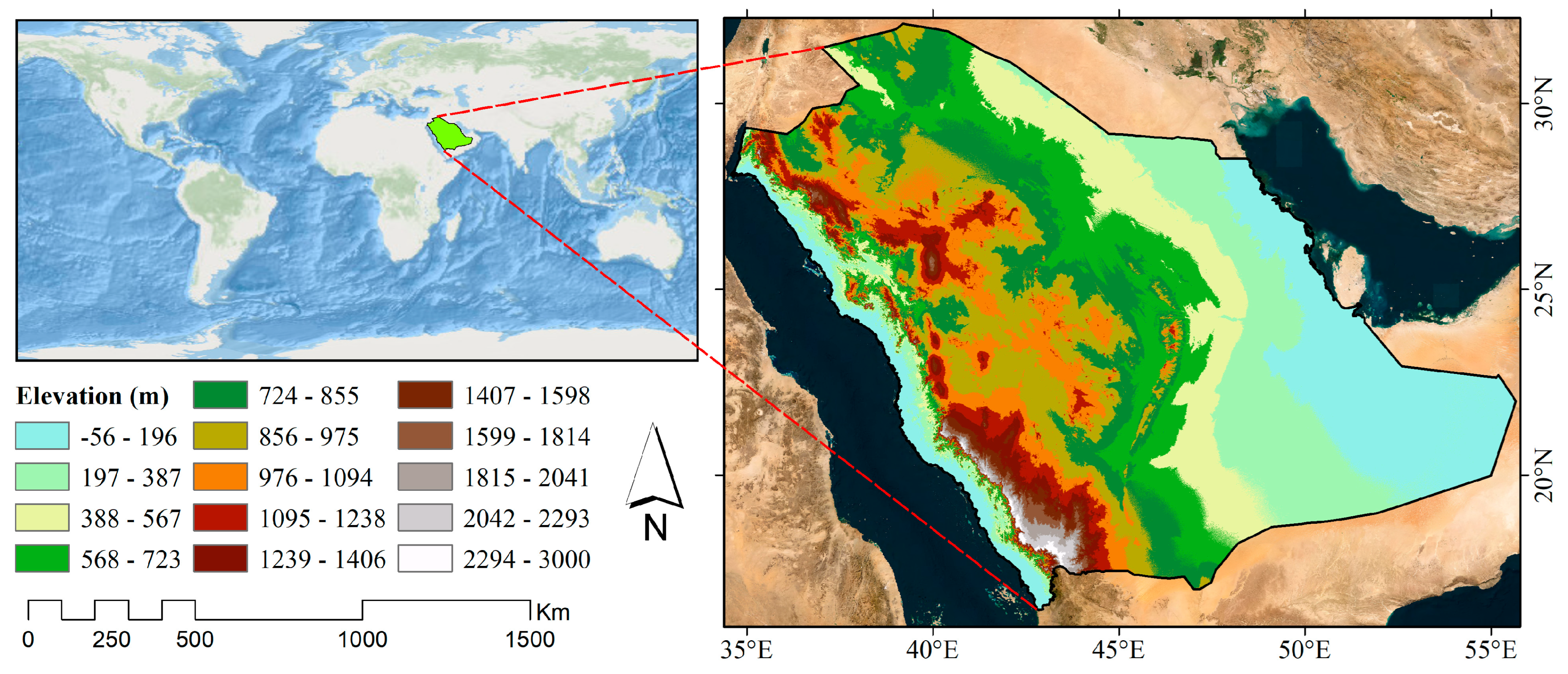
This research covers 75% of the Kingdom of Saudi Arabia (KSA), excluding the Empty Quarter due to the lack of available rain gauges. KSA is located between (16.4°:32.1° N and 34.6°:55.6° E) as shown in Figure 1. KSA is divided into 13 provinces: (1) Al-Riyadh, (2) Holy Makkah, (3) Al-Madinah, (4) Al-Qaseem, (5) Eastern Region, (6) Asir, (7) Tabuk, (8) Hail, (9) Northern Borders, (10) Jazan, (11) Najran, (12) Al Baha, and (13) Al-Jouf, as shown in Figure 2A. This vast region spans approximately 2,150,000 square kilometers, constituting approximately 80% of the Arabian Peninsula’s land [66,67,68]. KSA has approximately 2800 km of coastline along the Red Sea and the Arabian Gulf, with both bodies of water serving as the main suppliers of water vapor for the country [69]. The Kingdom of Saudi Arabia is characterized by noticeable topographical diversity. It is classified into five distinct components: (I) relatively flat coastal plains at the Red Sea and Arabian Gulf shorelines; (II) Najd and Northern Plateaus extending over the majority of the central and northern regions of the kingdom; (III) Empty Quarter Desert in the southern part of the kingdom, which is known as the Rub’ al Khali and is considered the world’s largest sand desert, covered by immense, undulating sand-dunes with heights reaching 250 m [70]; (IV) the Tuwayq Mountains, situated within the central region of the Najd Plateau, which extend for 800 km from the border of the Rub’ al Khali in the south to the border of Al-Qasim in the north, attaining heights of up to 600 m [71]; (V) the Asir mountains, which are located in the southwestern part of KSA, characterized by steep slopes and containing the highest elevation in the country at the Al-Sawda peak where the altitude reaches about 3000 m above mean sea level [36]. The Kingdom of Saudi Arabia suffers from a shortage of freshwater sources and is considered the largest country in the world without any rivers. It primarily relies on rainfall and groundwater, as well as desalination of seawater, to meet the increasing demand for water due to population growth. Most of the rainfall in the kingdom falls in the winter season, especially between October and April [72]. Several climatic classifications describing rainfall scarcity in KSA can be found in the literature: desert, hyper-arid and arid [73], arid [74], and extremely dry [75]. Variability in KSA’s topography contributes to climatic and rainfall pattern diversity over the kingdom in terms of location, time, and intensity. The southeastern part of Saudi Arabia, which includes the Asir Mountains, is characterized by severe spatial changes in rainfall patterns due to the topographical complexity that generates orographic precipitation conditions [76,77]. It receives the highest rainfall depth in KSA with an average annual precipitation of up to 500 mm [73]. Figure 2B illustrates the spatial distribution of average annual rainfall depth over the period 1960 to 2018. The average value at each gauge is computed based on available records, and the spatial distribution is generated using the Inverse Distance Deterministic interpolation technique, between the points average values [78].

Figure 1.
Kingdom of Saudi Arabia location and topography.
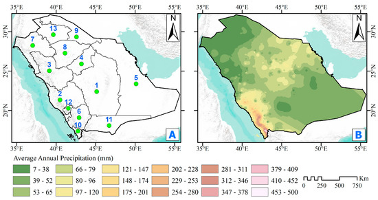
Figure 2.
(A) KSA administrative zones, (B) spatial distribution of mean annual precipitation from 1960 to 2018 [78].
2.2. Rain Gauges
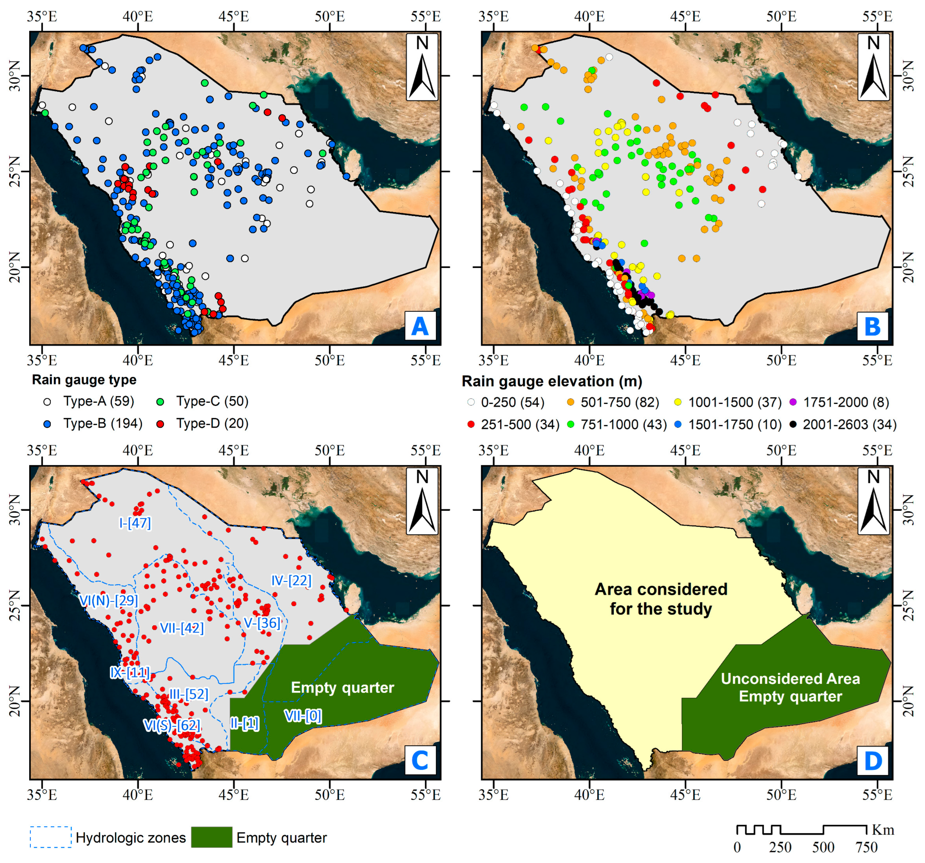
The most accurate and reliable source of rainfall data is terrestrial rain gauges. Therefore, assessing any proposed method or data source of precipitation depends on error assessment through comparison with ground measurements. In the current study, 323 rain gauge records were acquired from different authorities in KSA. These collected rain gauges are classified based on data type and recording methodology into four types: (A) Automatic recording of precipitation and other meteorological parameters, (B) Automatic recording of precipitation only, (C) Manually recorded precipitation data, and (D) Irregular manual rainfall recording times [79], as shown in Figure 3A. Due to the absence of information regarding the recording time for the 20 rain gauges of type D, they were omitted from the dataset, resulting in 303 stations being utilized for this study. The impact of KSA’s diverse topography, ranging from zero-altitude coastal plains to mountains with elevations up to 3000 m, was considered in the analysis of rain gauge data. Accordingly, the elevation of each rain gauge is considered a secondary parameter in the geostatistical Co-Kriging analysis. Figure 3B shows the variation in elevation of the rain gauges used. KSA is divided into nine hydrological zones [74]. The hydrological zones, along with the number of rain gauges contained within each, are shown in Figure 3C. The highlighted region, encompassing Zone VII and segments of Zones II and IV as depicted in Figure 3C, lacks any rain gauges. This region has been labeled as the “Empty Quarter” because it nearly encompasses its geographic boundaries. It has been excluded from the study area due to the absence of ground data available for satellite data assessment or conducting geostatistical analysis. Figure 3D shows the extent of the current study area.
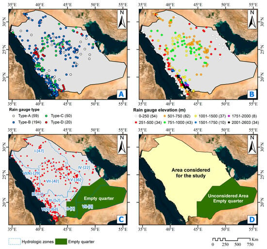
Figure 3.
(A) Rain gauge type, (B) elevations of rain gauges used in the current study, (C) KSA hydrological zones and number of contained gauges, (D) the extent of the current study.
2.3. Satellite Data
Seven satellite precipitation datasets (sources shown in Table 1) were downloaded and used in the current study:
CHIRPS V2.0 depends on the infrared radiation emitted by Cold Clouds in the upper atmosphere for specific Duration (CCD) rainfall estimations [80,81]. The TMPA 3B42 V7 algorithm and interpolated gauge products are utilized to fine-tune the CCD rainfall estimates [82,83,84,85]. CHIRPS is an almost-worldwide spatial resolution dataset that spans the region between north and degrees south [24]. The University of California at Santa Barbara (UCSB) provides CHIRPS precipitation data in monthly, decadal, pentadal, and daily intervals, spanning the period from 1981 to the near present [86].
PERSIANN datasets were developed by the Center for Hydrometeorology and Remote Sensing at the University of California, Irvine, utilizing Gridded Satellite (GridSat-B1) IR data [87]. The precipitation dataset is generated by utilizing Artificial Neural Networks to treat remotely-sensed satellite data [88]. PERSIANN spans the region between north and south [89]. Three PERSIANN datasets are utilized in the current study.
- PERSIANN dataset which is available in hourly, 3-hourly, 6-hourly, daily, monthly, and annual temporal resolution from March 2000 to the near present with spatial distribution.
- PERSIANN-CDR dataset which is available in daily, monthly, and annual temporal resolution from January 1983 to the near present with spatial distribution.
- PERSIANN-CCS dataset which is available in hourly, 3-hourly, 6-hourly, daily, monthly, and annual temporal resolution from January 2003 to the present with spatial distribution.
CMORPH provides bias-corrected precipitation estimates by utilizing the Climate Prediction Center (CPC) Morphing Technique to treat Passive Microwave (PMW) precipitation data [80]. The precipitation datasets are available in (30-min/8 km), (hourly/), and (daily/) spatiotemporal resolutions. The daily precipitation data used in the current study extends from north to south with a time coverage starting from Jan-1998 to the near present.
TMPA 3B42 is a collaborative mission between NASA and the Japan Aerospace Exploration Agency (JAXA), to study tropical and subtropical precipitation. The TRMM Multi-satellite Precipitation Analysis algorithm (TMPA) is utilized in the processing of the low-orbit five-sensor satellite data [85], to provide precipitation datasets. Two versions of TMPA datasets are available: 3B43 and 3B42, for daily and sub-daily (3-h) temporal resolution, respectively. Both datasets are available in spatial resolution and span the region between north and degrees south [28]. TMPA 3B42 is available in two versions: V6 and V7. V7 has a significant improvement in accuracy over V6 [29,30,31,32,33]. Accordingly, TMPA 3B42 V7 was selected for the current study. The TMPA 3B42 V7 dataset has a time coverage from January 1998 to January 2020.
GPM IMERG is a part of the collaborative NASA-JAXA Global Precipitation Measurement (GPM) mission. It employs an international network of satellites to provide worldwide precipitation and snowfall observations [90]. GPM IMERG exhibits greater sensitivity compared to TRMM in detecting light rain with an intensity of less than 0.5 mm/h [91]. The GPM algorithms utilize a sophisticated Dual-frequency Precipitation Radar (DPR) and a multi-channel GPM Microwave Imager (GMI) integrated into a Core Observatory Satellite. This satellite serves as a benchmark for standardizing various operational satellite measurements [92]. GPM IMERG V7 has a global coverage span from north to south with degree spatial resolution. It has several temporal resolutions (30 min, 3 h, daily, 7 days, and monthly) [93]. Each dataset has three runs classified based on product latency: A- (Early Run, 4-h latency), B- (Late Run, 14-h latency), and C- (Final Run, 3.5-month latency). The GPM IMERG V7 Final Run precipitation dataset is available from 1 June 2000 to the near present. Figure 4 shows the temporal coverage and resolution of each SPD.
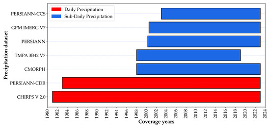
Figure 4.
The temporal coverage for each Satellite Precipitation Dataset.
2.4. Interpolation of Ground Station Data
Spatial interpolation methods utilize scattered measured points to build a surface of the studied variable that covers the study area. Spatial interpolation techniques are classified into two major approaches: (A) geostatistical and (B) deterministic approaches [94]. The deterministic approach handles measured data through a conventional interpolation approach to produce a parametric function used to obtain the missing values. Contrarily, the geostatistical approach deals with the problem of missing spatial data from the probabilistic perspective [95]. The details of deterministic and geostatistical techniques are given in Appendix B.
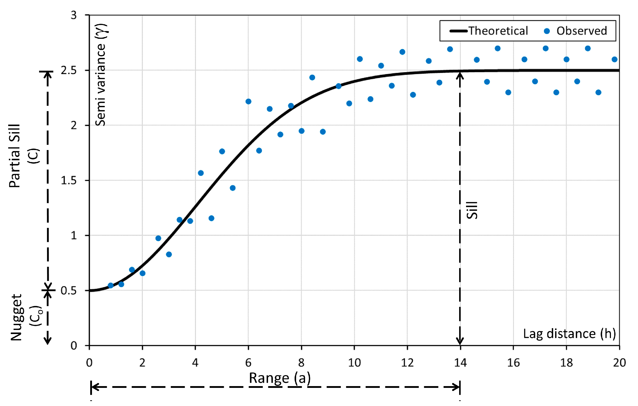
Geostatistical interpolation techniques, like deterministic interpolation techniques, are methodologies to obtain inferences about spatially varied parameters. The core difference between the two techniques is that the geostatistical technique considers the spatial variability of the studied parameters [96,97]. The semivariogram has a pivotal role in geostatistical interpolation since it provides a link between spatial description and spatial prediction. In all geostatistical interpolation techniques, the semivariogram provides a measure of dissimilarity (variability) between the investigated variables’ measured data in both space and direction [98]. It is calculated as one-half of the average squared difference between the values of all possible pairs of data separated by a lag vector , as given in Equation (1) and shown in Figure 5. Several theoretical semivariograms are fitted to observed measurements to provide a mathematical presentation of the variance. In the current study, seven theoretical variogram models are selected for evaluation, namely Circular, Spherical, Exponential, Gaussian, K-Bessel, J-Bessel, and Stable, as shown in Equations (2) through (8), respectively, in Table 2 [52].
where:
- are the measured values at locations , respectively.
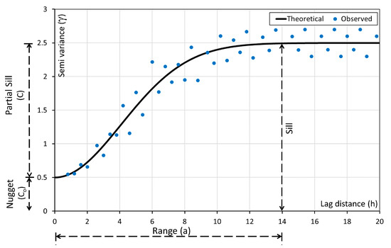
Figure 5.
Main parameters of typical semivariograms.
Figure 5.
Main parameters of typical semivariograms.
Where:
- : Semivariance at distance h
- The range is the distance between two measured values that, when exceeded, the semivariogram is flattened and the two points are no longer correlated.
- The nugget is the value of variance in a very short distance.
- The sill is the maximum variance located at a distance .
- The partial sill is the difference between the sill and the nugget values.

Table 2.
Semivariogram models.
Table 2.
Semivariogram models.
| Model | Equation | ||
|---|---|---|---|
| Circular | (2) | ||
| Spherical | (3) | ||
| Exponential | (4) | ||
| Gaussian | (5) | ||
| K-Bessel | (6) | ||
| J-Bessel | (7) | ||
| Stable | (8) | ||
Where:
- is a value found numerically so , for any ,
- are the gamma functions (),
- is the modified Bessel function of the second kind of order [99]
- is a value found numerically so , for any ,
- is the J-Bessel function [99].
- is a stability parameter ranging from 0 to 2.
In the current study, due to the nature of total annual and maximum daily rainfall where continuity is assured at small distances, all semivariogram nugget values were set to zero. This assumption also implies that the effect of measurement error is negligible [100,101]. After obtaining the theoretical semivariogram parameters, geostatistical techniques can be used to estimate the missing values. Equation (9) illustrates the general concept of geostatistical spatial estimation of a missing variable at the location .
where:
- : the estimate of the variable of interest at the location.
- the measured value of the variable of interest at the location.
- the weight of .
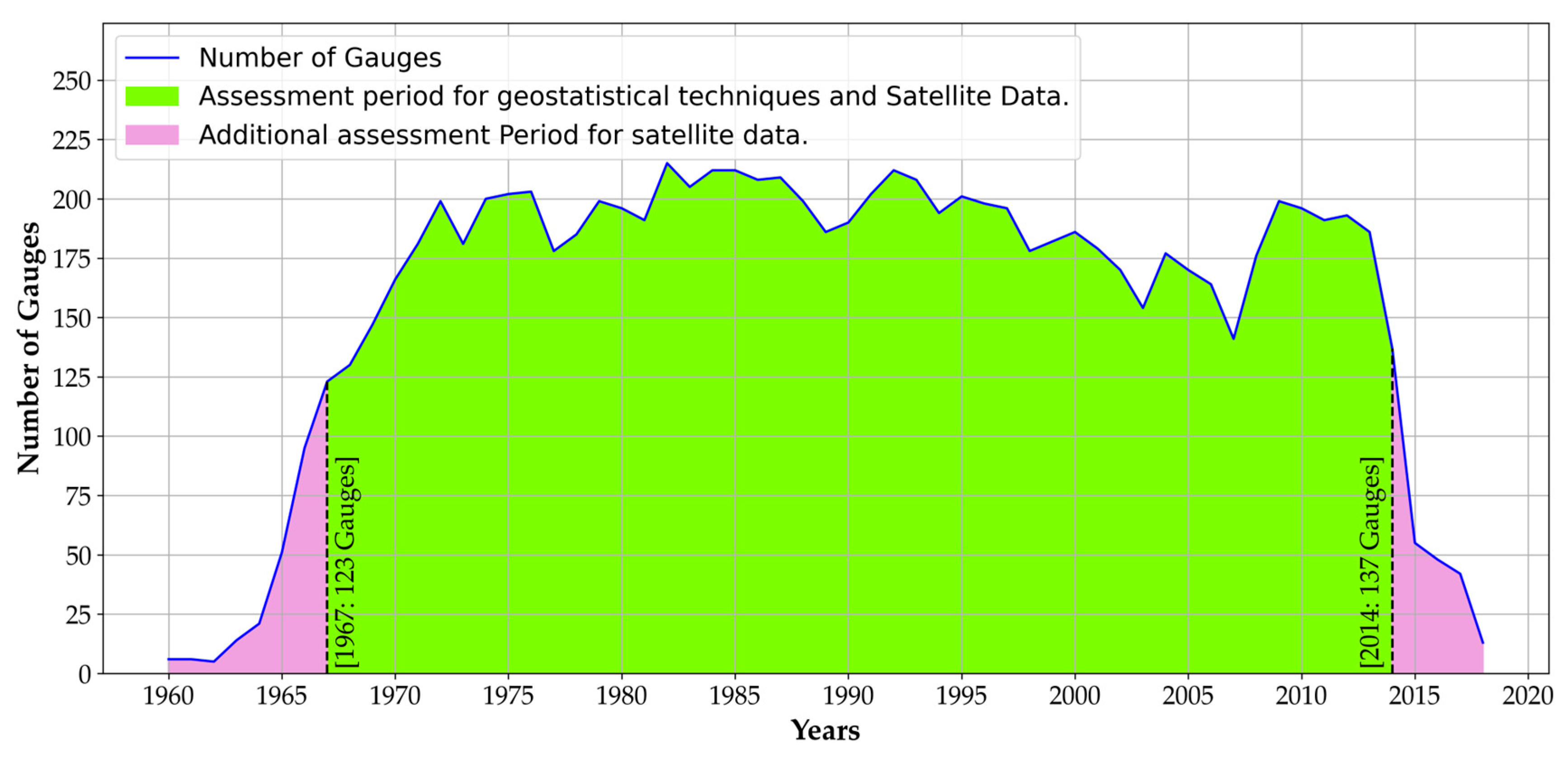
As concluded in the literature, the geostatistical approach yields more precise outcomes compared to deterministic methods. Accordingly, forty-two geostatistical model alternatives were generated using different Kriging and Cokriging models alongside nine semivariogram models, in addition to the Empirical Bayesian Kriging as given in Table 3. The number of available terrestrial gauge records varies significantly from year to year, as given in Figure 6.

Table 3.
Matrix of geostatistical method application codes employed in the present study.
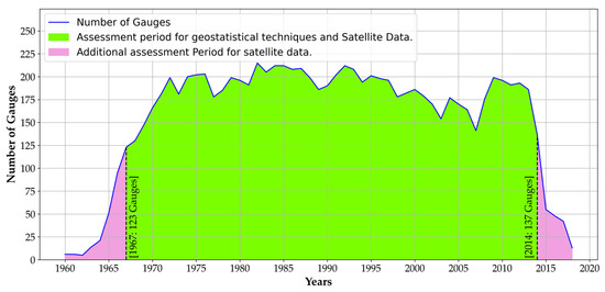
Figure 6.
Variation in the number of available rainfall gauge records across KSA from 1960 to 2018.
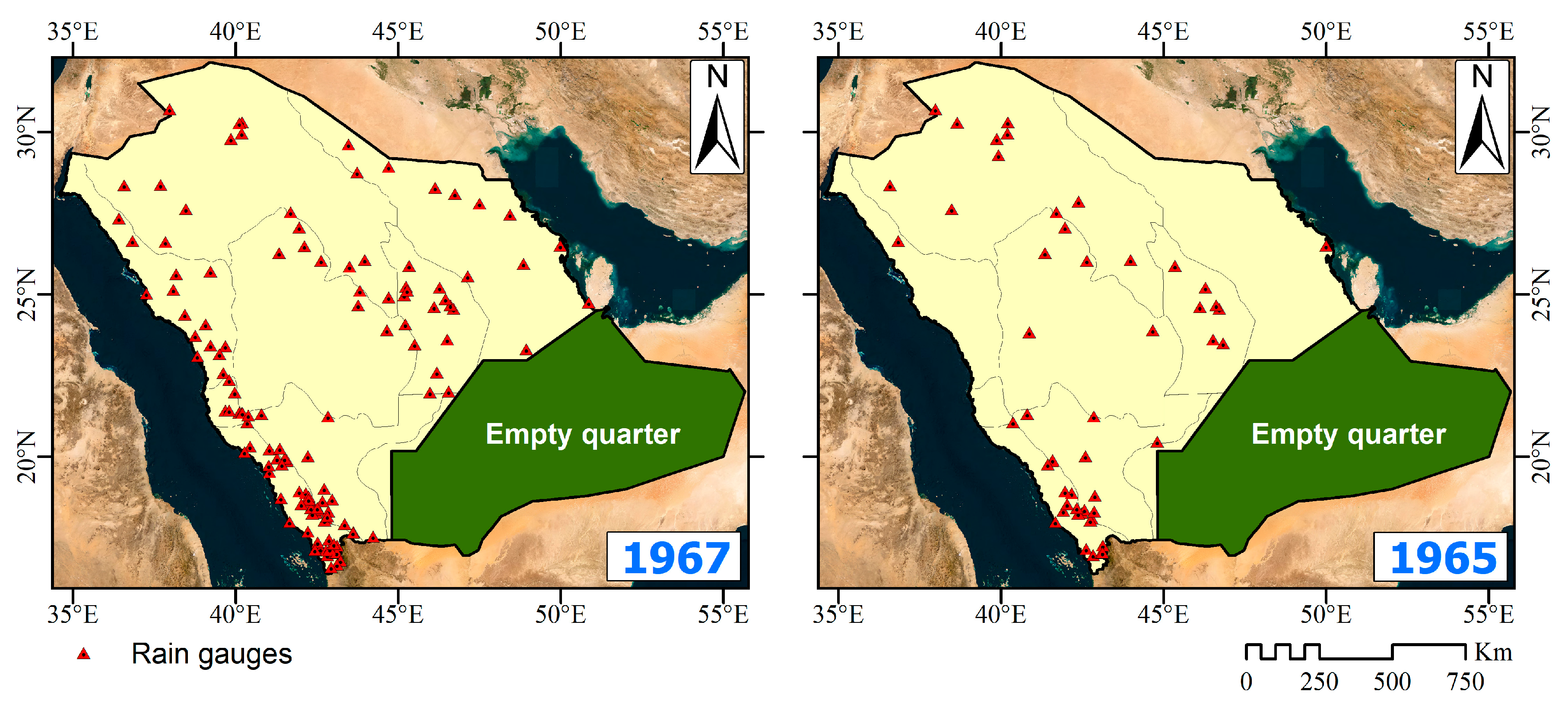
No specific thresholds were identified in the literature regarding the minimum required spatial density of rain gauges for the appropriate application of geostatistical techniques. Based on the quartile analysis of the number of terrestrial rain gauges available from 1960 to 2018, years with rain gauge records of less than 62 records per year were excluded from the geostatistical analysis. For the current study, the geostatistical analysis was conducted from 1967 to 2014, with a minimum 123 rain gauge records per year. Figure 7 shows the distribution of terrestrial gauges for an excluded year (1965, with 50 gauges) and the year with the lowest density of rain gauges among those considered (1967, with 123 gauges).

Figure 7.
Rain gauge spatial distribution across KSA in 1965 (50 gauges) and 1967 (123 gauges).
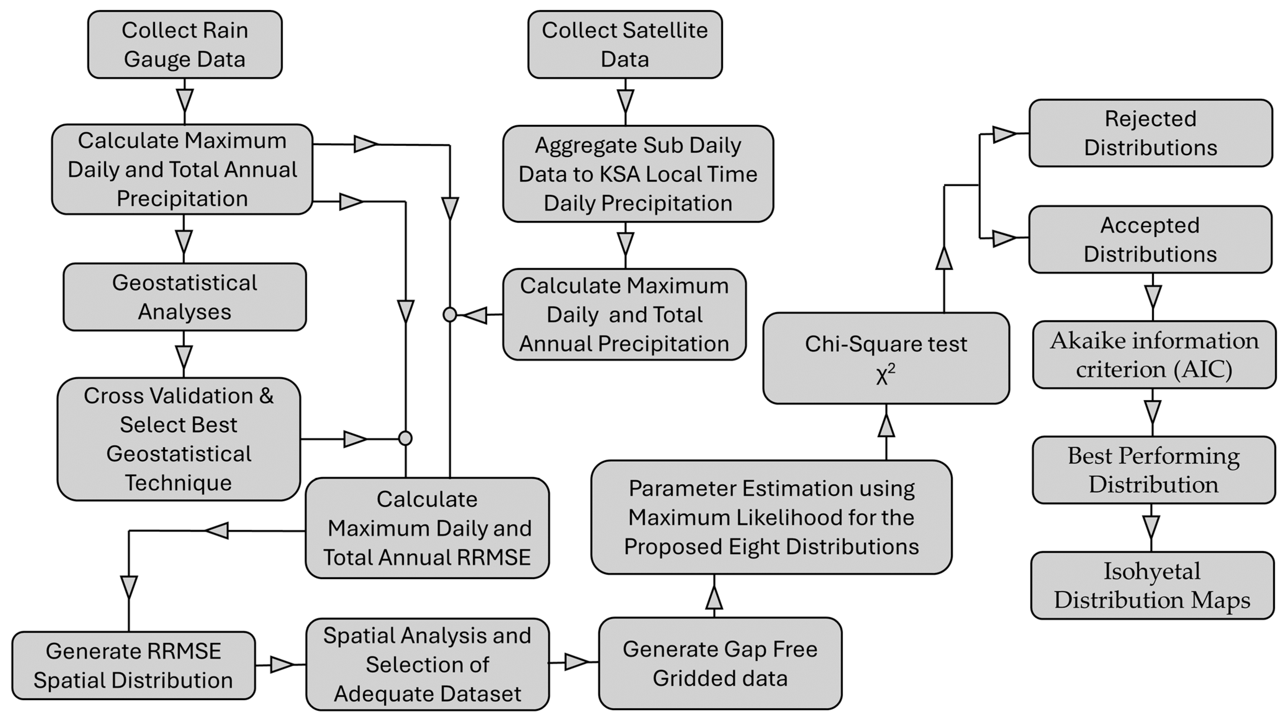
Figure 8 summarizes the procedure followed in the current study, starting from data collection and ending with the generation of isohyetal maps of maximum daily precipitation for the various return periods.

Figure 8.
Flow chart for producing gap-free precipitation data.
3. Results and Discussion
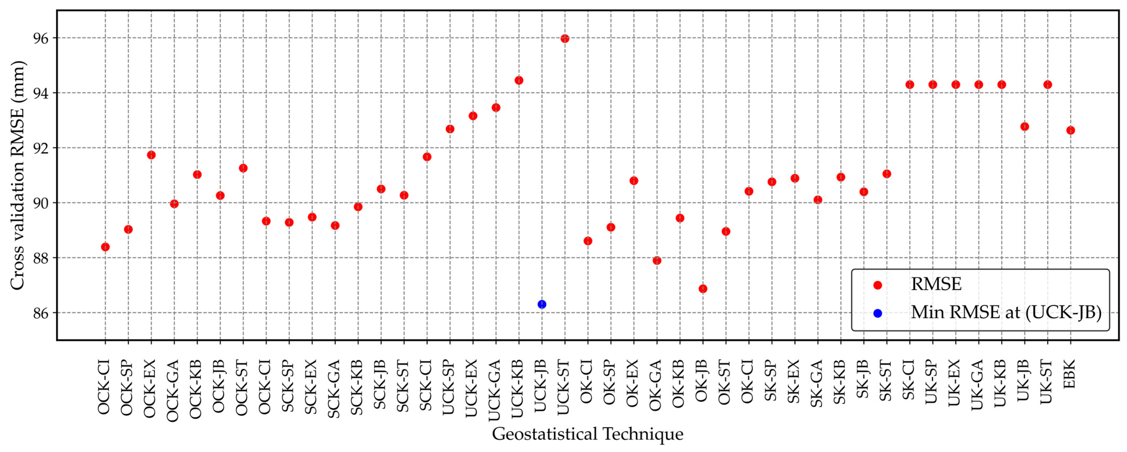
The geostatistical analysis is applied annually from 1967 to 2014 with a minimum of 123 gauges records per year. Cross-validation [100,102,103] is applied to each measured value within the study area, where each data point is removed, one at a time, and a predicted value at the removed point location is estimated using the remaining measured points with the geostatistical technique under assessment. The cross-validation Root Mean Square Error (RMSE) is computed as given in Equation (10). In the current study, the cross-validations RMSE is utilized as a selection tool to pick the most appropriate geostatistical technique among the 43 techniques proposed. Figure 9 illustrates the variation of the cross-validation RMSE with geostatistical techniques for total precipitation over the study area in 1999 as an example. The lowest cross-validation RMSE value was achieved while using Universal Cokriging with a J-Bessel semi-variogram (UCK-JB). Similarly, OCK-CI is selected for maximum daily precipitation in 1999 as shown in Figure 10. UCK-JB and OCK-CI are utilized to generate the spatial distribution of total annual precipitation and maximum daily precipitation, respectively, in 1999.
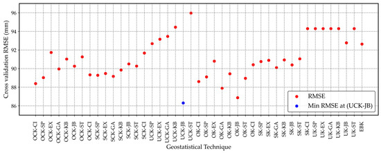
Figure 9.
Variation of the cross-validation RMSE with geostatistical techniques for the total precipitation depth over the study area in 1999.
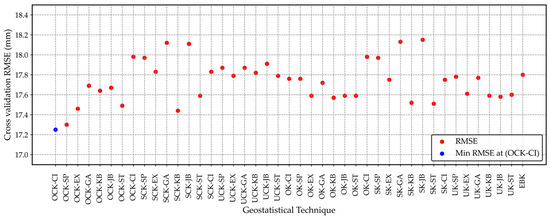
Figure 10.
Variation of the cross-validation RMSE with geostatistical techniques for the maximum daily precipitation depth over the study area in 1999.
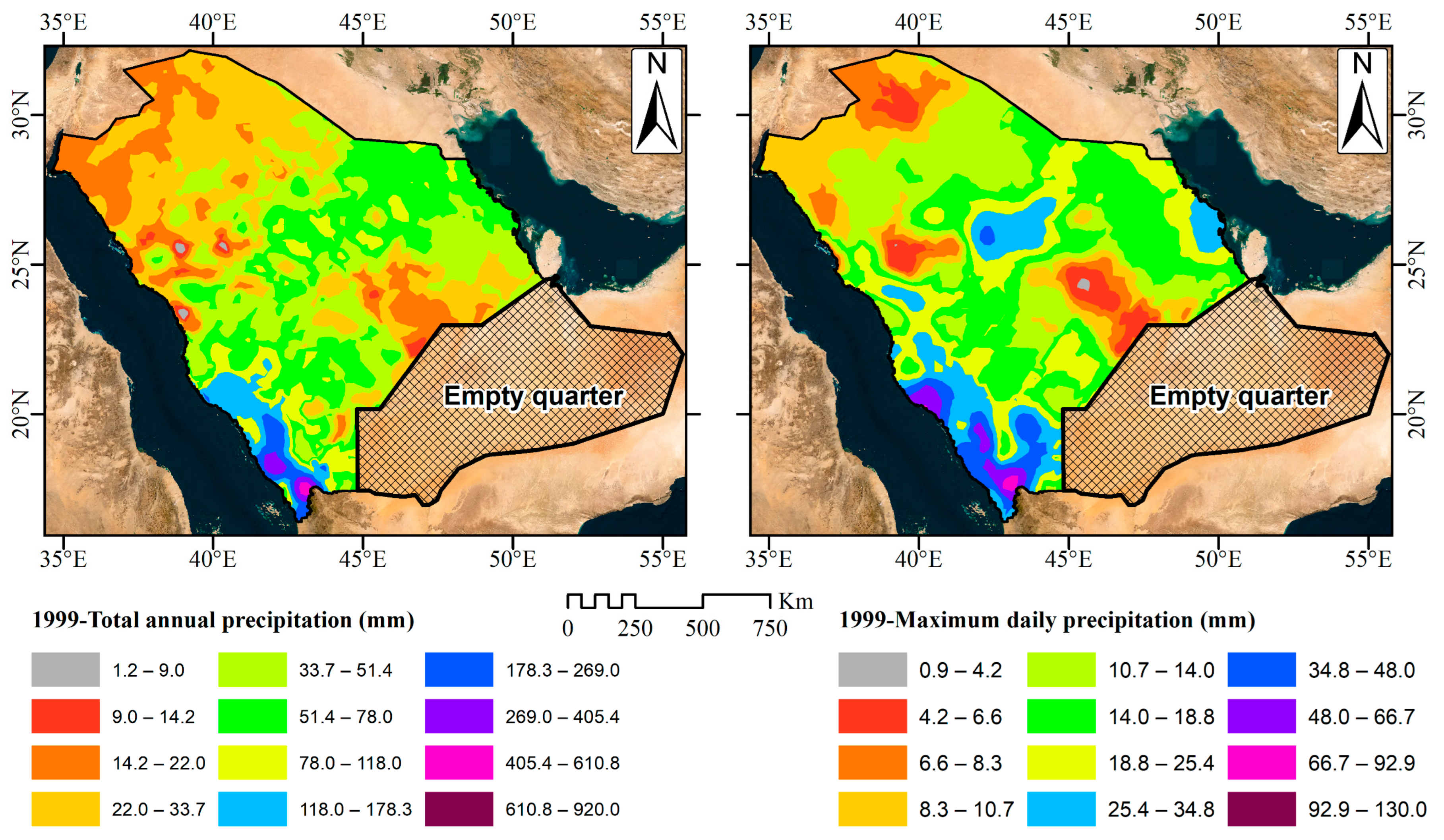
Figure 11 shows the spatial distribution of total annual and maximum daily precipitation depth in 1999 using the selected OCK-CI and UCK-JB geostatistical techniques, respectively. Due to the randomness of missing rainfall data and the variability in precipitation depth from one year to another, no specific approach can be considered as a generally recommended geostatistical technique for the study area. The analysis conducted for the 1999 dataset is replicated across other precipitation datasets spanning from 1967 to 2014 to discern the optimal geostatistical techniques with the least root mean square error (RMSE).
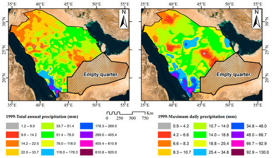
Figure 11.
Spatial distribution of the total annual and maximum daily precipitation in 1999 using geostatistical techniques (UCK-JB and OCK-CI, respectively).
Table 4 presents the superior geostatistical techniques for both total annual and maximum daily precipitation depths observed from 1967 to 2014, determined based on the lowest cross-validation RMSE. Notably, it is observed that the geostatistical technique yielding the lowest RMSE for the total annual precipitation dataset generally differs from that for the maximum daily precipitation dataset. This variation is attributed to differences in the variograms employed for each dataset, stemming from disparities in their respective variances.

Table 4.
Selected geostatistical methods for maximum and total annual precipitation depth.
Furthermore, the Supplementary Materials include isohyetal maps depicting the spatial distributions of total annual and maximum daily precipitation depth across the study area from 1967 to 2014, utilizing the identified best geostatistical techniques. These Supplementary Materials are anticipated to provide valuable resources for researchers and engineers, allowing direct utilization of these maps without the necessity of re-conducting the data gap analysis.
The subsequent phase involves evaluating the utilization of various satellite rainfall datasets to address data gaps and comparing them with the previously discussed geostatistical techniques. To accomplish this objective, it is imperative to ensure consistency in the timing of the daily rainfall measurements, in terms of both commencement and termination, between the ground-based data and the satellite data. This alignment is crucial to enable a fair and accurate comparison with the available ground rainfall data.
As per the daily precipitation bulletin released by the KSA Ministry of Environment, Water, and Agriculture, the recorded daily precipitation depth is the accumulated rainfall depth from 9:00 a.m. to 9:00 a.m. of the next day (KSA local time). Satellite precipitation datasets (SPDs) are reported in Coordinated Universal Time (UTC). KSA local time is 3.00 h ahead of UTC, as shown in Figure 12A. The SPDs are reported at the starting time of the rainfall accumulation interval. The accumulation interval differs according to the temporal resolutions of the SPDs. In the current study, daily, 3 h, and 30 min SPDs were used, as illustrated in Figure 12B. The SPDs with 3 h of temporal resolution are aggregated from UTC 06:00 to UTC 03:00 of the following day to achieve daily records matching KSA gauges. The 30 min datasets are aggregated from UTC 06:00 to UTC 05:30 of the following day. Exact time matching between the SPDs data and daily rain gauge records could not be achieved for datasets with daily temporal resolution (CHIRPS V2.0 and PERSIANN-CDR).
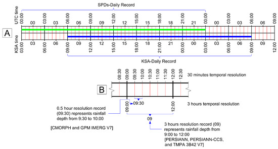
Figure 12.
(A) Times for reported data of SPDs based on UTC and KSA local times, (B) sample of dataset names and temporal coverage.
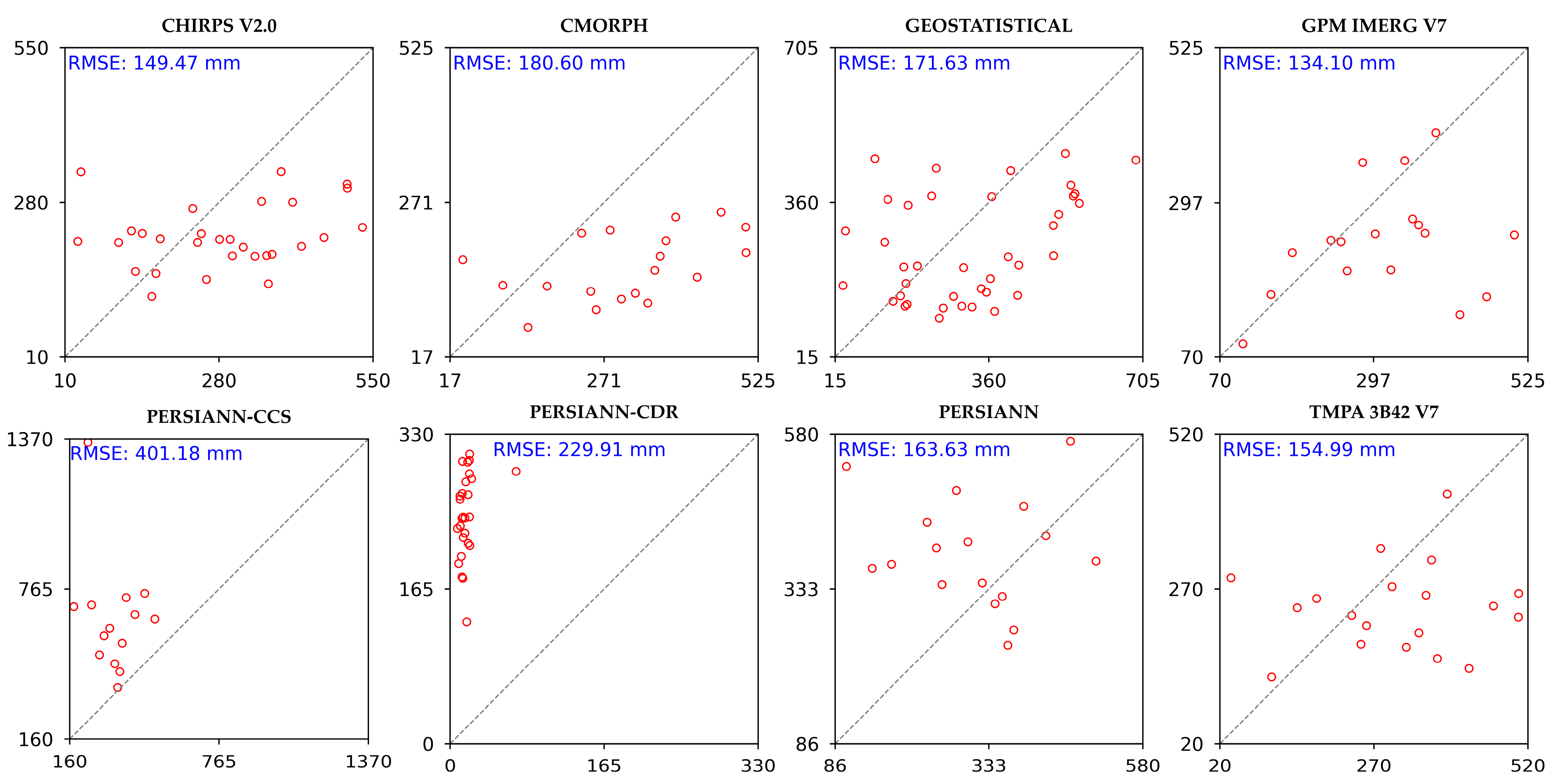
The common approach to evaluating the quality of fitting between the predicted rainfall depth (whether from satellite data or geostatistical techniques) and the terrestrial rain gauge observations is the RMSE (also called Root Mean Square Deviation) given by Equation (11). In the current study, the RMSE has a millimeter dimension similar to the studied variable (precipitation). Each terrestrial gauge with measured values is compared to the eight predicted precipitation depths—seven SPDs and the geostatistical method—for both maximum and total annual precipitation. As an example, Figure 13 and Figure 14 show the variation of the RMSE for rain gauge SA166 for the eight evaluated datasets. Figure 13 and Figure 14 clarify the variation in the number of overlapped points used for RMSE calculation for each dataset, using gauge SA166 as an example. Consequently, the RMSE cannot be utilized to select the best-performing datasets for maximum daily and total yearly precipitation. In this study, the Normalized Root Mean Square Error (NRMSE) is proposed as a replacement for the RMSE to account for the variation in the number of overlapped readings. The Normalized Root Mean Square Error (NRMSE) is the normalized form of the RMSE by the mean value as given in Equation (12). NRMSE is used to replace the RMSE in comparing the adequacy of different datasets.
where:
- and are the predicted values and average value of the variable respectively.
- n/; is the number of records.
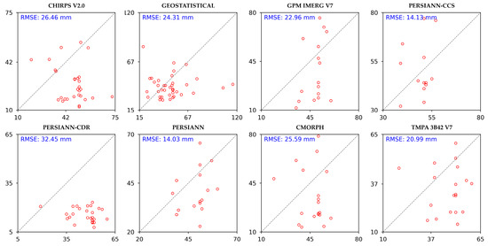
Figure 13.
Variation of RMSE for maximum daily data sources at gauge SA116 (terrestrial rain gauge records on the horizontal axis and predicted data on the vertical axis in mm). The numbers of overlapped annual records are 29, 39, 16, 13, 26, 16, 19, and 19 years of records for CHIRPS V2.0, Geostatistical, GPM IMERG V7, PERSIANN-CCS, PERSIANN-CDR, PERSIANN, CMORPH, and TMPA 3B42 V7, respectively.
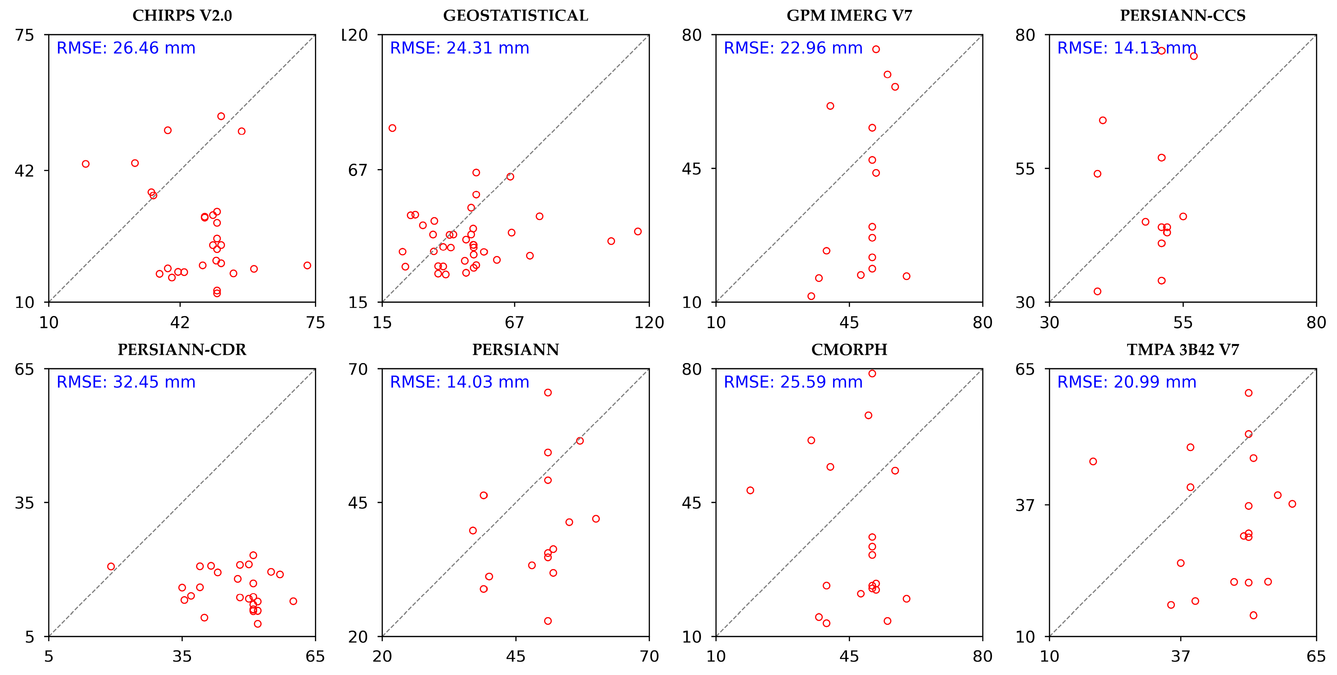
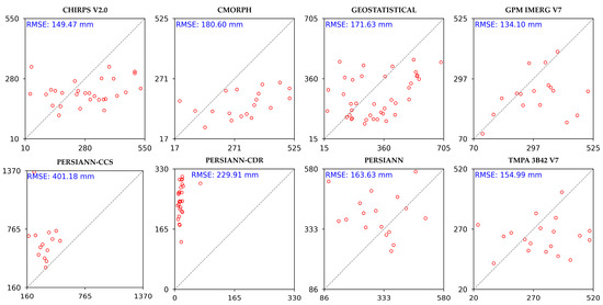
Figure 14.
Variation of RMSE for total annual data sources at gauge SA116 (terrestrial rain gauge records on the horizontal axis and predicted data on the vertical axis in mm). The numbers of overlapped annual records are 29, 39, 16, 13, 26, 16, 19, and 19 years of records for CHIRPS V2.0, Geostatistical, GPM IMERG V7, PERSIANN-CCS, PERSIANN-CDR, PERSIANN, CMORPH, and TMPA 3B42 V7, respectively.
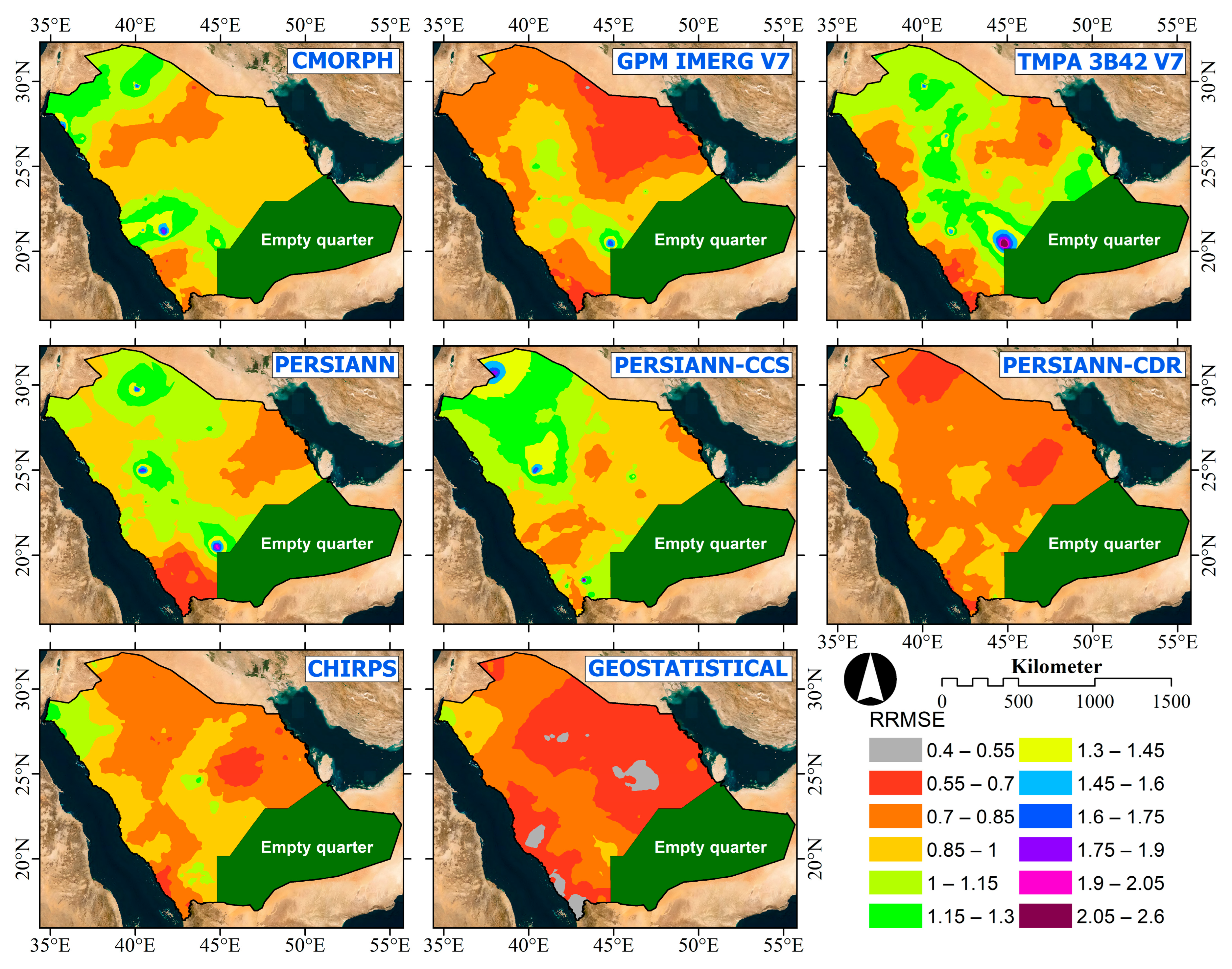
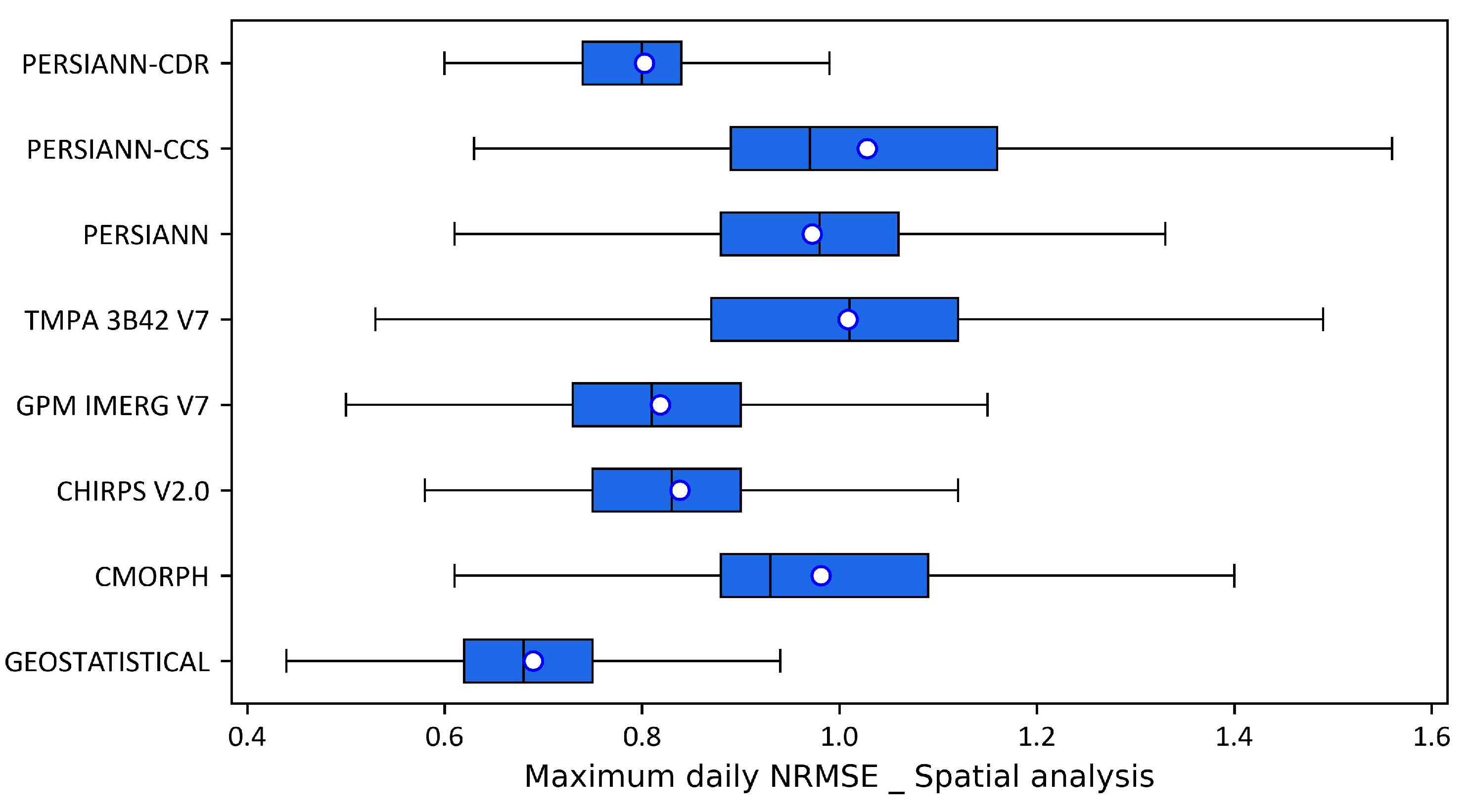
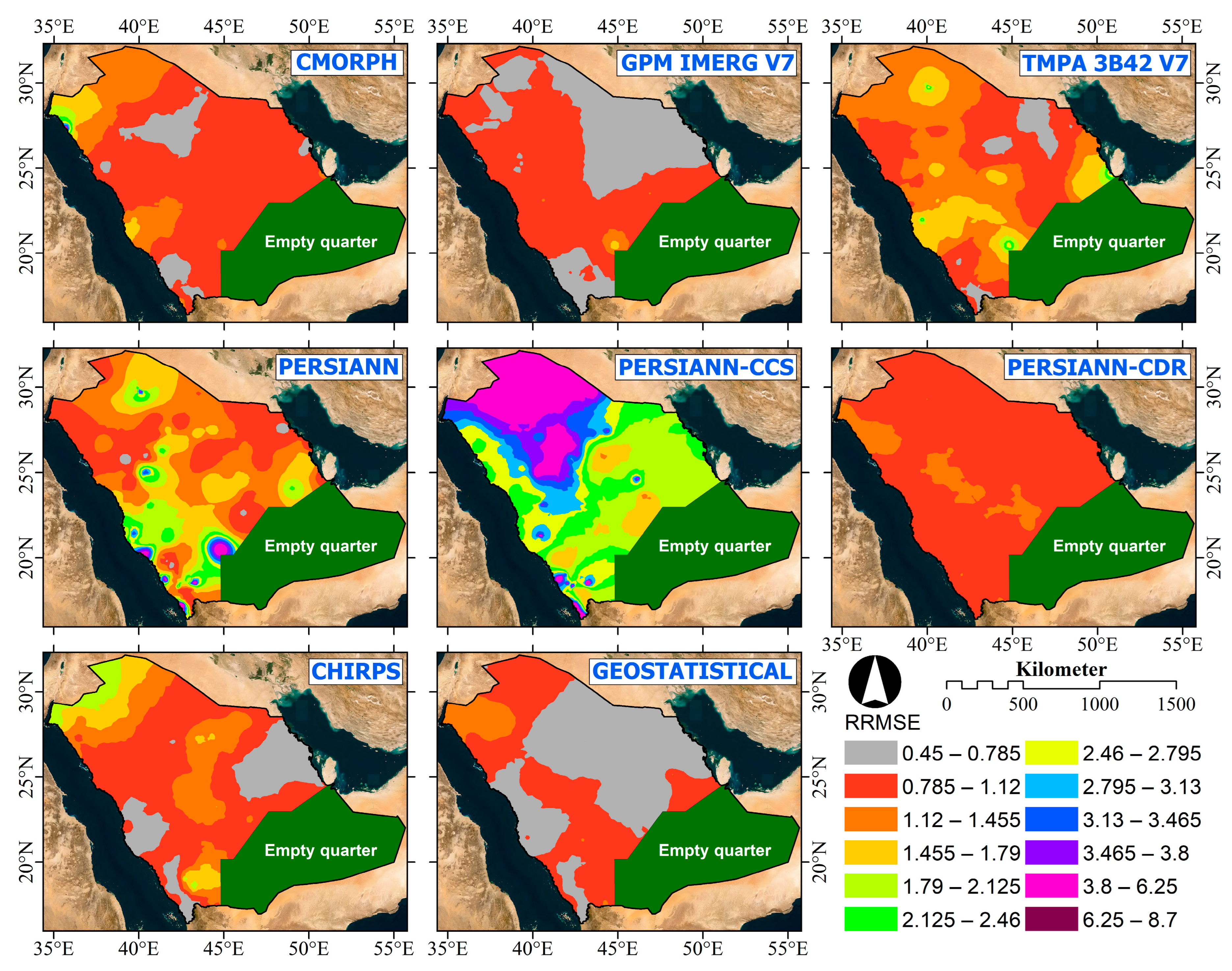
The derived Normalized Root Mean Square Error (NRMSE) metrics are calculated at terrestrial rain gauge locations where measured data are accessible. As the distribution of rain gauges across the study area is uneven, characterized by a concentration of gauge stations in the southwestern region, a moderate density in the central area, and sparse coverage in other regions (refer to Figure 4), it is anticipated that this nonuniform distribution will influence the computed NRMSE values. Employing Inverse Distance Weighting (IDW) techniques, the spatial distribution of NRMSE values is generated to mitigate the impact of rain gauge distribution irregularity on assessment accuracy. Figure 15 illustrates the resultant spatial distribution of NRMSE values, while a summary of spatial analyses, depicted through Box-Plot charts, is presented in Figure 16 for the case of maximum daily precipitation. Analogously, NRMSE values corresponding to total annual precipitation, along with their characteristics, are delineated in Figure 17 and Figure 18, respectively. These figures distinctly demonstrate the superior performance of geostatistical analysis over satellite datasets based on NRMSE values.
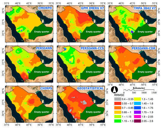
Figure 15.
The spatial variation of NRMSE for the maximum daily precipitation case.
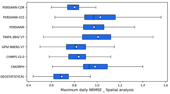
Figure 16.
Characteristics of NRMSE for different maximum daily precipitation datasets.

Figure 17.
The spatial variation of NRMSE for total annual precipitation.
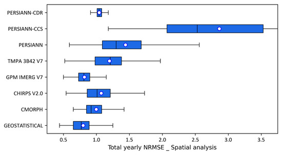
Figure 18.
Characteristics of NRMSE for different total yearly precipitation datasets.
The geostatistical approach yielded minimum mean NRMSE values of 0.69 and 0.80 for maximum daily precipitation and total annual precipitation cases, respectively. Despite the PERSIANN-CCS satellite dataset possessing the highest spatial resolution (4 km × 4 km) among the tested precipitation satellite datasets, it exhibited the lowest performance in both maximum and total annual precipitation estimation. Notably, the GPM IMERG V7 dataset outperformed other satellite precipitation datasets in estimating total annual precipitation, with an average spatial NRMSE value of 0.82, compared to 0.80 achieved by the geostatistical technique. Conversely, for the estimation of maximum daily precipitation, the PERSIANN-CDR dataset displayed the highest performance, with an average spatial NRMSE value of 0.80, as opposed to 0.69 obtained by the geostatistical approach. It is noteworthy that the optimal performance of the geostatistical technique is observed in the southwestern (Asir and Makkah regions) and central (Al-Riyadh region) areas, coinciding with the regions boasting the highest density of rain gauges.
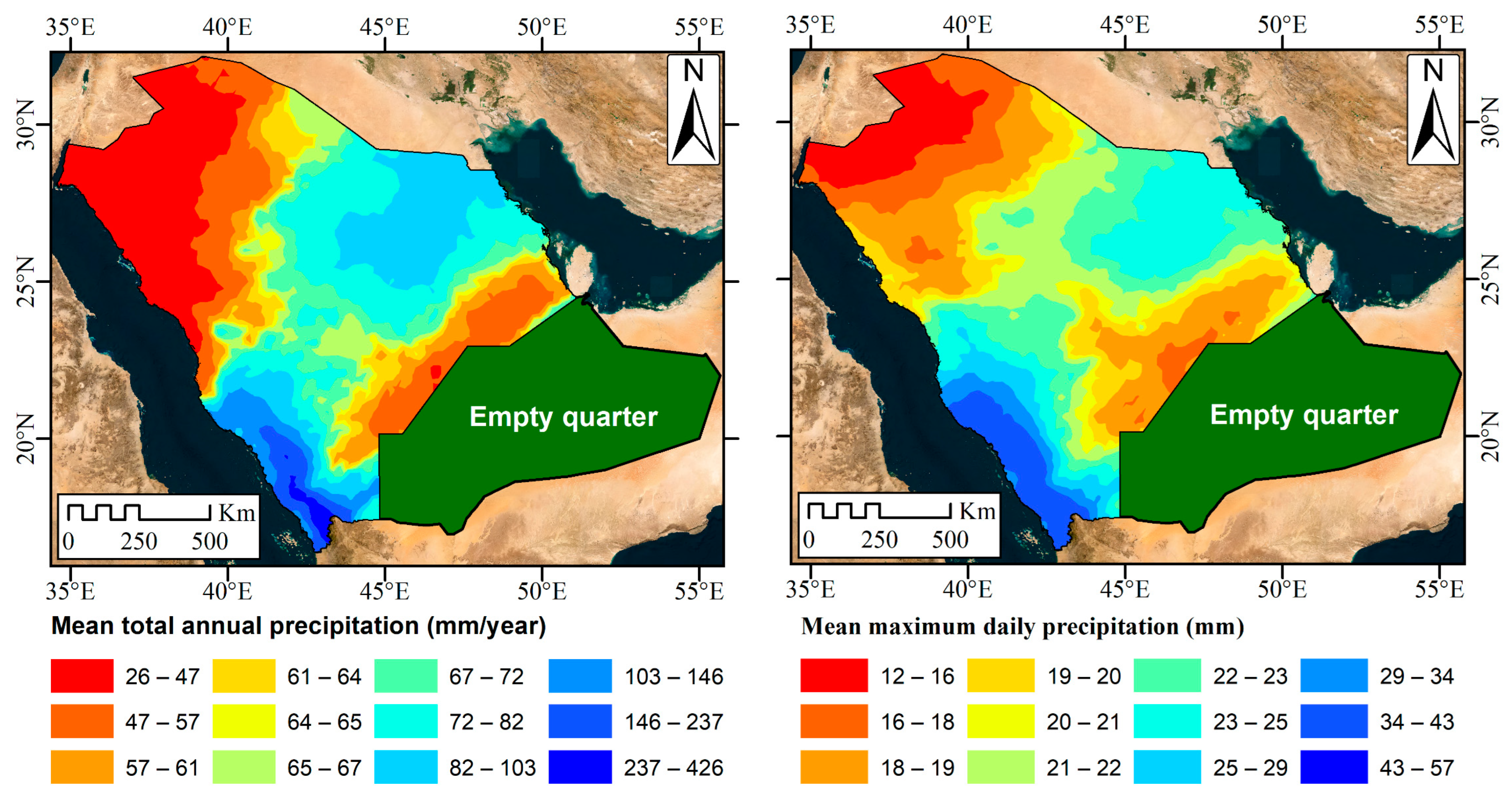
In light of the aforementioned findings, the geostatistical technique was implemented, following the recommendations outlined in Table 4, to obtain the spatial distribution of maximum daily and total annual precipitation across the Kingdom of Saudi Arabia (KSA) and to generate corresponding isohyetal contour maps for both cases on an annual basis spanning the period from 1967 to 2014. Supplementary Materials contain these datasets and maps. As a result of this spatial distribution analysis conducted on an annual basis, the mean total annual and maximum daily precipitation depths are depicted in Figure 19.
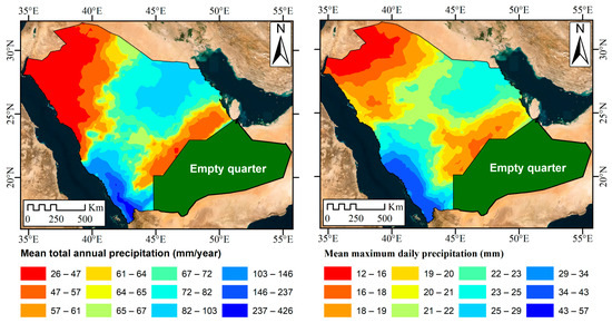
Figure 19.
Mean total annual and maximum daily precipitation depths over the study area (based on precipitation data from 1967 to 2014, and also Table 4 recommendations).
As an illustration of the utility of the generated maps, the geostatistical layers produced for Maximum Daily Precipitation Depth (MDPD) (presented in the Supplementary Materials) can be utilized to furnish a gap-free MDPD time series at any gauge station. Figure 20 exemplifies the filled gaps in the maximum daily rain gauge data for station A110. Subsequently, the gap-free time series records can serve as inputs for frequency analysis to obtain the MDPD corresponding to different return periods. Generating isohyetal maps for MDPD for various return periods necessitates the application of geostatistical techniques between frequency analysis outcomes at gauge locations. To minimize geostatistical interpolation error, gridded precipitation data are generated with a spacing of 4470 m in both east and north directions, providing a maximum served area of 20 square kilometers for each grid point. The selection of the 20 square kilometer limit is based on the World Meteorological Organization (WMO) recommendation of a minimum of one rain gauge per every 20 square kilometers in urban areas [11]. Following the WMO limit, the study area encompasses 71,790 grid points utilized in generating MDPD raster layers for different return periods without any geostatistical interpolation and with a resolution of 20 square kilometers per pixel.
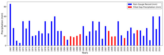
Figure 20.
Filled precipitation data for station A110 as an example.
Several statistical probability distributions can be used in the frequency analysis [55]. In the process of generating raster layers for extreme values of Maximum Daily Precipitation Depth (MDPD) corresponding to various return periods, a range of statistical probability distributions is evaluated, including the Gamma, Normal, and Extreme values distribution families, as elaborated in Table 5.

Table 5.
Evaluated Statistical Distributions.
Each statistical distribution is characterized by a probability density function (PDF), given by Equations (13) through (20). Parameters for each distribution are selected to optimize the likelihood of observations, employing the Method of Maximum Likelihood (MLK), as articulated in Equation (21). Subsequently, the Chi-square test is employed at a significance level of 5% to assess the adequacy of the tested distribution. Data is partitioned into (k) classes, as specified by Equation (22), and the comparison between the calculated as given in Equation (23) and critical values, with degrees of freedom, determines the acceptance or rejection of the PDF for predicting MDPD across different return periods.
where:
- is the number of observations, and equals 48 in the case of gap-filled data series.
- is the number of observations in the class interval i.
- is the expected number of observations in the class interval (i) according to the tested PDF.
Furthermore, the Akaike Information Criterion (AIC) [104] serves as a criterion for selection among accepted probability density functions subsequent to the Chi-square test. AIC, being an asymptotically unbiased estimator, is calculated for the evaluated PDF model according to Equation (24), leveraging the known value of the log-likelihood function.
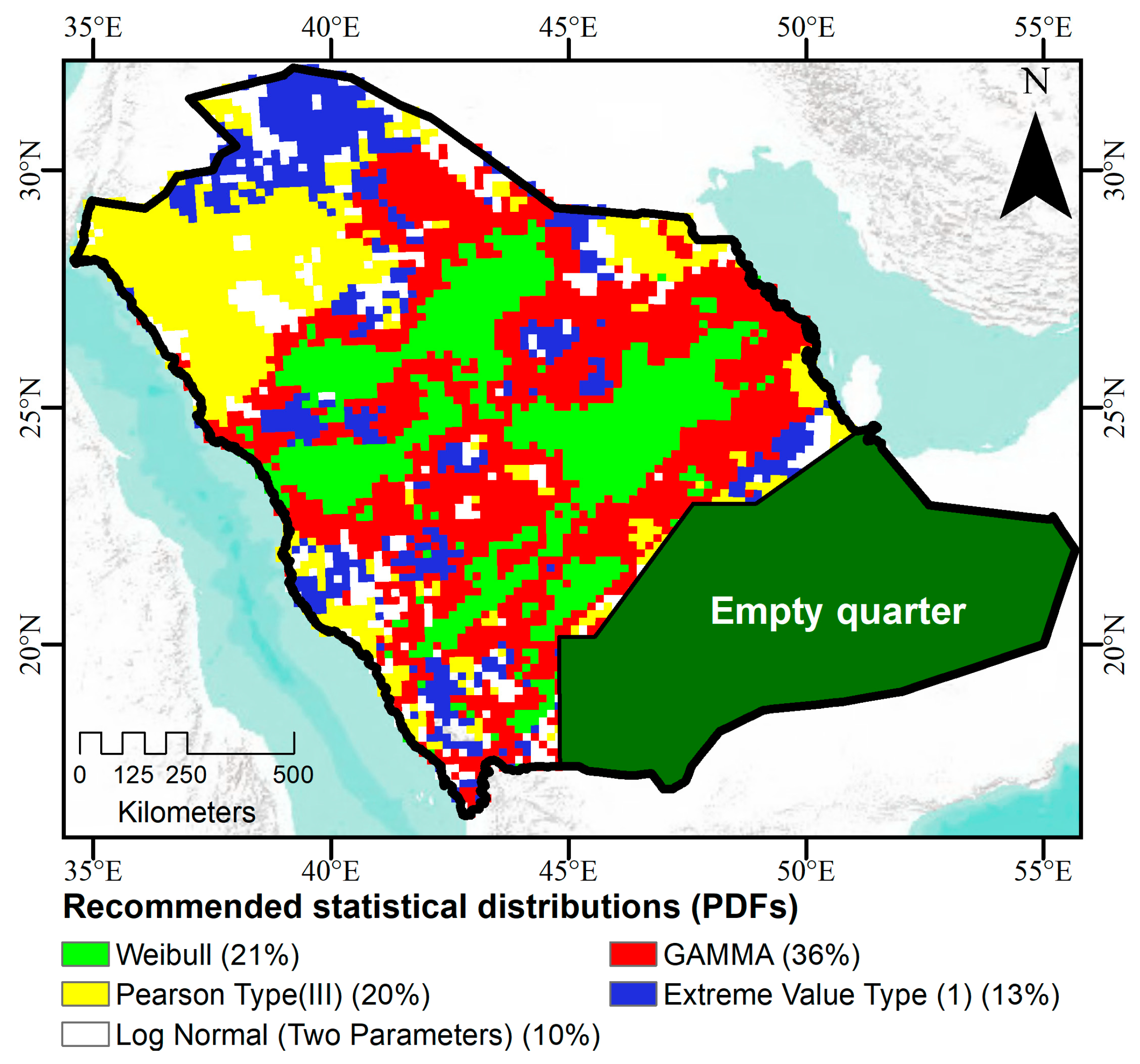
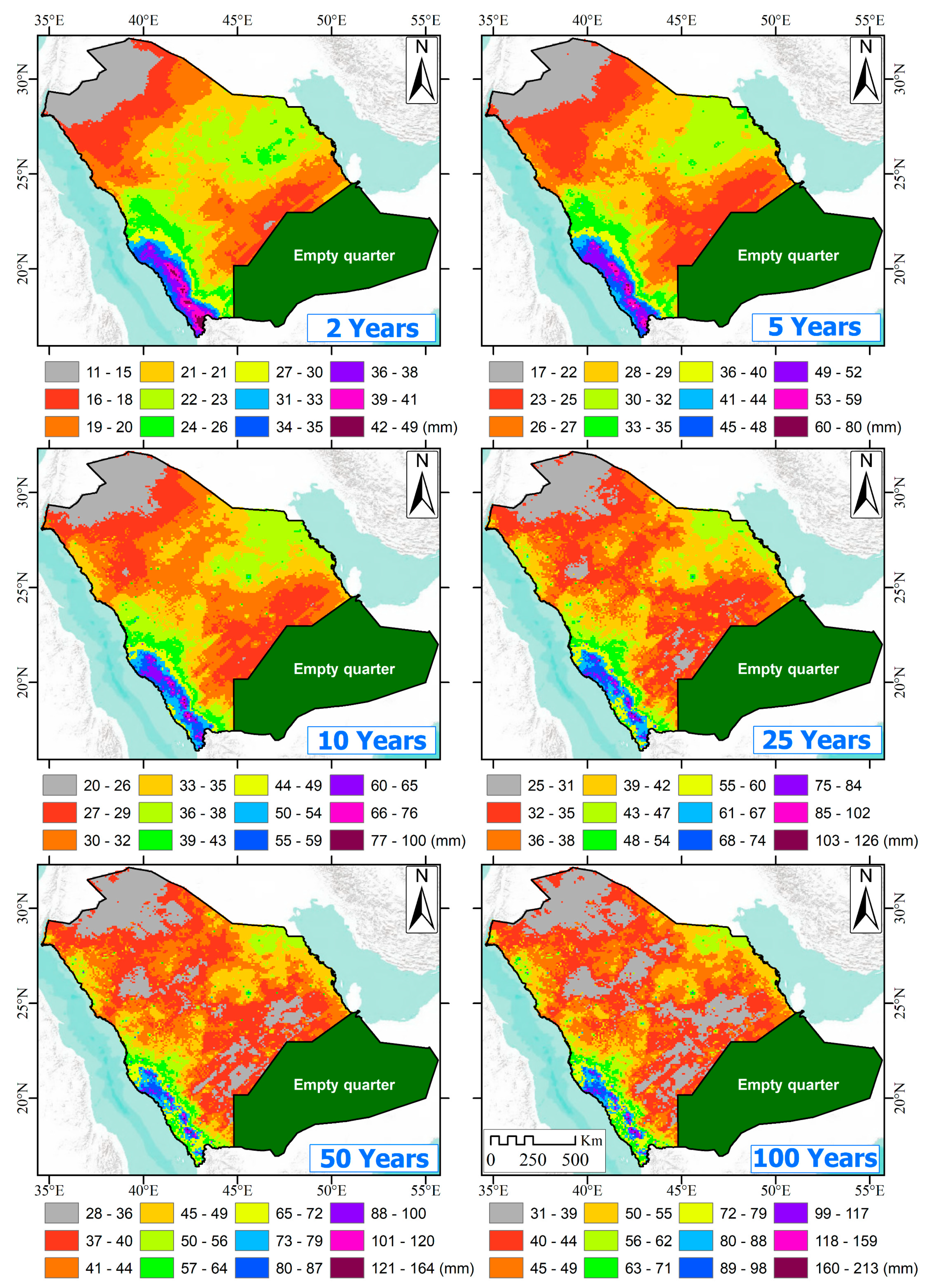
Figure 21 presents a raster map summarizing the PDF with the lowest AIC at each grid point, thereby indicating the spatial distribution of the selected PDF. The dominance of Gamma family distributions is evident, covering approximately 56% of the study area, followed by Extreme value distributions with 34% coverage, and lastly, the Normal distribution family with 10% coverage. Isohyetal maps for maximum daily precipitation across different return periods are computed and delineated in Figure 22, based on the recommended PDF identified in Figure 21.
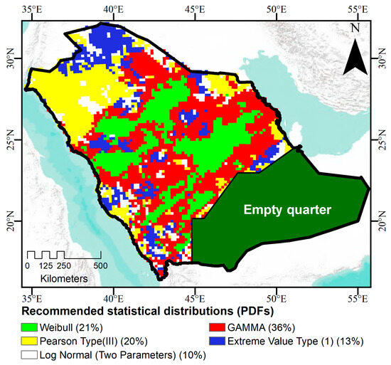
Figure 21.
Recommended statistical distributions (PDFs) for MDPD and area coverage percentage.
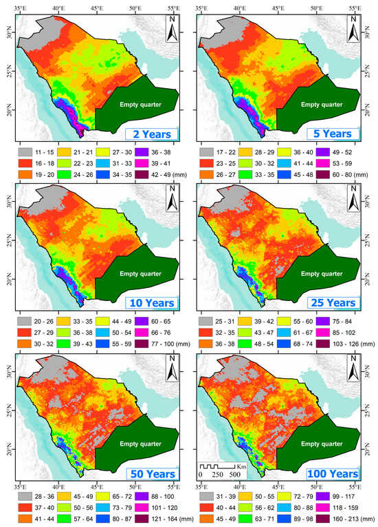
Figure 22.
The spatial variation of MDPD for different return periods.
4. Conclusions
This comprehensive study addresses the critical need for accurate and gap-free rainfall data in arid regions, employing the Kingdom of Saudi Arabia (KSA) as a focal case study. It covers 75% of the Kingdom of Saudi Arabia’s area and spans the period from 1967 to 2014. The remaining 25% of the KSA’s area is omitted due to the lack of rain gauge coverage. The research evaluated seven satellite precipitation datasets and 43 geostatistical interpolation techniques to compensate for deficiencies in terrestrial rain gauge records.
Normalized Root Mean Square Error by the mean value of observation (NRMSE) is employed as a ranking criterion for the evaluated datasets. Geostatistical techniques demonstrated superior performance over satellite datasets, particularly achieving NRMSE values of 0.69 and 0.80 for maximum daily and total annual records, respectively. Notably, regions with higher gauge density exhibited the best performance.
Among satellite datasets, PERSIANN-CDR and GPM IMERG V7 demonstrated superior accuracy, with NRMSE values of 0.80 and 0.82 for maximum and total annual records, respectively. Geostatistical techniques were further applied to generate spatial distributions of maximum and total annual precipitation, revealing their efficacy in addressing data gaps.
Probability Density Functions (PDFs) from the Gamma, Extreme Value, and Normal distribution families were assessed to fit the gap-filled datasets. These families exhibited best fitting over 56%, 34%, and 10% of the study area gridded data, respectively. The selected PDF at each grid point was then utilized to compute maximum daily precipitation for various return periods, facilitating the creation of isohyetal raster maps for hydrological studies.
The rainfall dataset produced herein holds considerable value for professionals engaged in water resource and flood hazard assessments within Saudi Arabia, owing to several key advantages: (i) comprehensive coverage of the entire KSA region, excluding the Empty Quarter; (ii) utilization of 48 years of ground rain gauge records spanning the period from 1967 to 2014; (iii) mitigation of data gaps through integration of seven distinct Satellite Precipitation Datasets (SPDs) alongside the geospatial dataset, which exhibited the least error among its counterparts; (iv) inclusion of maximum daily and total annual rainfall data, as well as extreme events corresponding to various return periods. Notably, the latter dataset holds significant importance for informing decisions regarding flood hazard assessment and protective measures.
While the focus of this study may appear geographically restricted to Saudi Arabia, its significance transcends national borders. By providing a robust framework for addressing data gaps through geospatial algorithms, this study serves as a guiding resource for engineers and researchers involved in flood protection and water resource management projects across KSA. The generated raster maps offer invaluable assistance in expediting the process of filling rainfall data gaps and identifying suitable statistical distributions. Moreover, the insights gleaned from this study hold relevance beyond the confines of KSA, offering valuable methodologies applicable to similar studies globally. However, it is imperative to acknowledge and address certain requirements and limitations when applying this approach in other case studies:
Firstly, temporal consistency is crucial. The availability of ground rainfall data from gauges covering the same time period and maintaining consistent data resolution (e.g., daily, monthly, annual) is essential for reliable analysis.
Secondly, the spatial distribution of ground gauges is pivotal. A sufficient quantity of gauges dispersed across the area of interest, rather than clustered or aligned in a specific direction, enhances the robustness of the interpolation process. Quality data from multiple gauges enriches the accuracy of the results.
Thirdly, consideration of local environmental factors is paramount. Understanding the influence of variables such as topography, prevailing winds, and proximity to large bodies of water aids in selecting appropriate interpolation methods and facilitates the interpretation of outcomes.
Lastly, it is important to acknowledge the potential impact of dynamic factors such as climate change on rainfall patterns. Geostatistical interpolation assumes spatial relationships between data gauges remain constant over time, which may not hold true in scenarios of significant climatic variability.
Supplementary Materials
The following supporting information can be downloaded at: https://www.mdpi.com/article/10.3390/w16070925/s1, Table S1: Characteristics of available rain gauges, Figure S1: Spatial distribution of maximum daily precipitation depth from 1967–1972, Figure S2: Spatial distribution of maximum daily precipitation depth from 1973–1978, Figure S3: Spatial distribution of maximum daily precipitation depth from 1979–1984, Figure S4: Spatial distribution of maximum daily precipitation depth from 1985–1990, Figure S5: Spatial distribution of maximum daily precipitation depth from 1991–1996, Figure S6: Spatial distribution of maximum daily precipitation depth from 1997–2002, Figure S7: Spatial distribution of maximum daily precipitation depth from 2003–2008, Figure S8: Spatial distribution of maximum daily precipitation depth from 2009–2014, Figure S9: Spatial distribution of total annual precipitation depth from 1967–1972, Figure S10: Spatial distribution of total annual precipitation depth from 1973–1978, Figure S11: Spatial distribution of total annual precipitation depth from 1979–1984, Figure S12: Spatial distribution of total annual precipitation depth from 1985–1990, Figure S13: Spatial distribution of total annual precipitation depth from 1991–1996, Figure S14: Spatial distribution of total annual precipitation depth from 1997–2002, Figure S15: Spatial distribution of total annual precipitation depth from 2003–2008, and Figure S16: Spatial distribution of total annual precipitation depth from 2009–2014.
Author Contributions
A.M.H.: conceptualization, data collection, data analysis, methodology, visualization, writing—review & editing. M.I.F.: project administration, R.H., M.A.M. and L.C.: reviewing of original draft and addressing of reviewers’ comments, M.H.E.: funding acquisition, review, editing, and project supervision. All authors have read and agreed to the published version of the manuscript.
Funding
This work was supported and funded by the Deanship of Scientific Research at Imam Mohammad Ibn Saud Islamic University (IMSIU) (grant number IMSIU-RG23109).
Data Availability Statement
Data will be made available on request.
Acknowledgments
The authors would like to express their sincere gratitude to Prof. Dr. Khaled H. Hamed for his invaluable technical support in programming and data processing throughout this research. His expertise and dedication greatly contributed to the success of this project. We are truly thankful for his assistance.
Conflicts of Interest
The authors declare that they have no known competing financial interests or personal relationships that could have appeared to influence the work reported in this paper.
Appendix A

Table A1.
Sample of satellite-borne datasets assessment studies.
Table A1.
Sample of satellite-borne datasets assessment studies.
| Study Type Location | Datasets | Gauges Study Accuracy | Study Period | Main Findings |
|---|---|---|---|---|
| Combined study Tapajos River basin—Amazon | TRMM 3B42 | 118 RG.&23 FG. Daily and Monthly | 1998–2006 for rain 2000–2003 for Flow | The TRMM estimates closely align with those obtained from the rain gauge record when averaged over the entire basin. The generated modeled hydrographs demonstrated acceptable accuracy, as evidenced by the comparison with 23 flow gauges within the basin [105]. |
| Statistical study Iran | TRMM 3B42 | Grid-1 Daily, Seasonal, Annual | 1998–2006 | The TRMM 3B42 data showed a weak correlation with daily records but displayed improved accuracy when assessing annual data. However, it tended to underestimate the average annual precipitation [106]. |
| Combined study Gilgel Abay basin-Ethiopia | CMORPH, TMPA 3B42RT, TMPA 3B42, PERSIANN | 4 RG.&1 FG. Daily and Monthly | 2006–2007 | Datasets utilizing microwave data (such as CMORPH and TMPA 3B42RT) consistently exhibit superior streamflow modeling, displaying a bias on the order of 53%. In contrast, the PERSIANN dataset, which relies on infrared data, demonstrates lower performance with a bias of 83%. Among these datasets, TMPA 3B42, which integrates both satellite and ground gauge data, exhibits the lowest performance, showing a bias of 8% [107]. |
| Statistical study China | PERSIANN-CDR | Grid-2 daily | 1983–2006 | PERSIANN-CDR effectively captured the spatial and temporal daily extreme rainfall characteristics, especially in the humid Manson region of eastern China. However, its performance notably diminished in arid and mountainous terrains, such as the Tibetan Plateau in the west and the Taklamakan Desert in the northwest [108]. |
| Statistical study 9 watersheds all over the world | 10 Datasets | 1052 RG. Daily, Monthly, Annual | 2000–2013 | The performance of satellite precipitation datasets is highly dependent on rainfall variability. Many datasets underestimate precipitation during wet seasons and overestimate it during dry ones [109]. |
| Statistical study Iraq | TRMM-3B42 | 4 RG. Monthly | 2000–2010 | A high correlation was observed between TMPA3B42 and ground stations at the monthly temporal scale. There was an overestimation of TRMM rainfall estimates recorded in most of the rainy months [110]. |
| Statistical study Iran | TMPA-3B42V7, PERSIANN, CMORPH | Grid-3 Daily and Monthly | 2003–2008 | TRMM TMPA 3B42 v7 demonstrates superior performance compared to the other two datasets across all the examined regions in Iran [111]. |
| Hydrological Gandak Himalayan River-China | TMPA 3B42 V7 | 5 FG.-Daily | 2000–2010 | The TRMM 3B42 dataset proves effective in hydrological modeling for rainfall intensities categorized as moderate to heavy (ranging from 7.5 to 124.4 mm/day). However, its performance is limited for both light rainfall (less than 7.5 mm/day) and extremely heavy rainfall (greater than 124.4 mm/day) intensities [112]. |
| Statistical study East India | IMERG V6, TRMM-TMPA-3B42 V7,GSMap V6 | Grid-4 Daily | June 2014 to September 2014 | Low correlation coefficients were reported between daily data and all datasets. IMERG and GSMap demonstrated superior performance compared to the TMPA dataset in detecting light rain events. Significant uncertainty is associated with all satellite-based precipitation products in regions characterized by orographic-dominated precipitation [113]. |
| Statistical study China | CHIRPS | Grid-5 Daily | 1981–2014 | CHIRPS exhibited superior performance during high-intensity rainfall events when contrasted with low-intensity rainfall in arid regions. Its accuracy is notably influenced by the movement of the monsoon. Additionally, CHIRPS datasets demonstrated better performance in the basins of southern China in comparison to those in northwestern and northern China [114]. |
| Statistical study KSA | GPM-IMERG (early, late, final) runs | 189 RG. Daily | October 2015 to April 2016 | The IMERG early run demonstrated satisfactory accuracy in the central, eastern, and certain western regions of KSA. However, notable fluctuations in accuracy were observed in other areas. Conversely, the final run exhibited improved accuracy in the southern and western regions but revealed higher errors in the northern and central parts [115]. |
| Statistical study China | TMPA-3B42V7, CMORPH-CRT, GPM-IMERG-V05B, GPM-IMERG-V04A | 542 RG. Daily, Seasonal, Annual | March 2014 to February 2017 | All datasets underestimated the depth of rainfall over the mountainous Tibetan Plateau and Xinjiang province, except IMERG V04A. IMERG V05B showed an improvement in rectifying the underestimation observed in IMERG V04A. IMERG demonstrated superior capabilities in detecting rainfall events compared to the other datasets. There is potential for enhancement in all datasets, especially in arid regions and high-altitude areas [116]. |
| Statistical study China | GPM IMERG (03, 04, 05) | Grid-6 Hourly and Daily | June 2014 to May 2015 | The final runs of IMERG V04 and V05 showed significant improvements compared to V03, except in the mountainous regions of the Tibetan Plateau and Xinjiang province [117]. |
| Statistical study KSA | PERSIANN-CDR, PERSIANN, TMPA-3B42, CMORPH | 29 RG. Daily and Monthly | 2003–2011 | All satellites exhibited superior performance during wet seasons compared to dry ones. Gauge-adjusted datasets (PERSIANN-CDR and TRMM 3B42) demonstrated a higher accuracy in detecting rainfall occurrences compared to the other unadjusted datasets [36]. |
| Combined study Meki and Ketar Basins-Ethiopia | CFSR, CHIRPS, PERSIANN-CDR, TMPA 3B42 V7 | 9 RG.&2 FG. Daily and Monthly | 1985–2004 | The CHIRPS dataset outperformed the other datasets in the statistical assessment of rainfall depth, as well as in the daily and monthly simulation of streamflow. Conversely, the reanalysis product CFSR exhibited the poorest performance, characterized by the highest mean error and relative biased ratio [118]. |
| Statistical study Egypt | GSMap, GPM-IMERG, CHIRPS | 29 RG. Daily | March 2014 to May 2018 | No consistent performance was observed among the tested datasets. CHIRPS exhibited the highest accuracy in predicting rainfall amounts [119] |
| Statistical study China | TMPA-3B42, GPM-IMERG | 830 RG. Daily | 2000–2017 | Both datasets captured the spatial pattern of extreme events, with an underestimation of extreme rainfall rates. The IMERG dataset demonstrated slightly better accuracy compared to the TMPA. The performance was notably superior in humid areas, while it showed a reduction in accuracy in arid and mountainous regions [120]. |
| Statistical study Upper Ganga River-India | TMPA 3B43 V7 | Grid-5 Monthly | 1998–2013 | TMPA underestimated precipitation amounts exceeding 400 mm and overestimated precipitation within the range of 100 to 370 mm. The correlation coefficients were higher during the post-monsoon and winter seasons compared to the pre-monsoon and monsoon seasons, with values of 0.65 and 0.57, respectively [121]. |
| Statistical study Mexico | CMORPH-CRT | 14 RG. 30 min and Daily | 2000–2018 | CMORPH-CRT exhibits a low to moderate correlation with rain gauge records, often associated with an overestimation of rainfall depth. Furthermore, CMORPH-CRT tends to overstate the frequency of precipitation events [122]. |
| Statistical study Zambezi Basin-South Africa | CMORPH | 66 RG. Daily, Weekly, Seasonal | 1998–2013 | The CMORPH dataset detects rainfall occurrences with 60% accuracy. It demonstrates higher precision during wet seasons in contrast to dry periods. Moreover, the predictive accuracy at a weekly temporal scale surpasses that of the daily scale [123]. |
| Statistical study Fincha & Neshe Basins-Blue Nile-Ethiopia | CHIRPS | 6 RG. Monthly, Seasonal, Annual | 1991–2015 | CHIRPS tends to overestimate precipitation in high-altitude regions while underestimating it in lower-altitude areas. Despite its coarse temporal resolution, which exceeds daily intervals, CHIRPS demonstrates satisfactory performance in satellite-based estimates of rainfall [124]. |
| Combined study Eastern Nile Basin-East Africa | TMPA-3B42V7 and CHIRPS | 35 RG.&3 FG Daily and Monthly | 1998–2007 | Although both datasets exhibit similar performance in terms of false alarm ratio (FAR), the TMPA 3B42 V7 demonstrates a higher probability of detection (POD) compared to CHIRPS. Both datasets yield satisfactory accuracy when simulating monthly discharge at the Blue Nile flow stations using the Hydro-Beam distributed hydrological model [125]. |
| Hyd. study Volta River basin-West Africa | 17 Datasets | 11 FG.-Daily | 2003–2012 | There is not a single precipitation dataset that can be considered the most effective for all hydrological processes. However, when it comes to evaluating daily streamflow, TAMSAT, CHIRPS, and PERSIANN-CDR exhibited the highest performance [126]. |
| Statistical study Bali Island | GSMap, IMERG, CHIRPS | 27 RG. Daily, Pentadal, Monthly, Seasonal | 2015–2017 | The datasets offer imprecise representations of the occurrence rates of light and heavy rainfall, defined as depths less than 1 mm per day and greater than 50 mm per day, respectively. Conversely, they tend to overestimate the frequency of moderate rainfall events, which range from 5 to 10 mm per day. Among the three datasets, IMERG demonstrated superior performance [127]. |
| Statistical study Shuaishui River Basin-China | GPM IMERG V6,TMPA 3B42V7 | 13 RG. Hourly, Daily, Monthly | 2009–2017 | The accuracy in estimating monthly precipitation was superior in both datasets compared to other temporal resolutions. The GPM dataset outperformed the TRMM dataset in estimating daily rainfall precipitation. However, neither dataset was able to satisfactorily estimate hourly rainfall [128]. |
| Statistical study Brazilian Amazonia | CHIRPS | 45 RG. Monthly and Annual | 1981–2017 | The CHIRPS datasets yield underestimated values for precipitation depth during the rainiest months. As a result, it was determined that CHIRPS is insufficient for accurately depicting rainfall trends in the study area [129]. |
| Statistical study Nigeria | 16 satellite precipitation estimates | 11 RG. Monthly | 2000–2012 | The precipitation estimates from IMERG-Final-V6 and Multi-Source Weighted-Ensemble Precipitation (MSWEP) v.2.2 demonstrated superior performance compared to other methods, thus making them the recommended choices for future hydrological studies [130]. |
| Combined study Ganjiang River Basin-China | TMPA 3B42, PERSIANN, CMORPH, CHIRPS | 36 RG.&9 FG Daily and Monthly | 1998–2014 for rain 2000–2014 for flow | CMORPH demonstrates the highest accuracy in capturing daily precipitation, while TMPA 3B42 exhibits the best performance in providing monthly precipitation data. Both datasets outperform PERSIANN and CHIRPS in capturing extreme precipitation events. Additionally, TMPA 3B42 yields the most accurate hydrologic model, as evidenced by the H17 streamflow results [131]. |
| Combined study West Rapti River basin-Nepal | PERSIANN-CCS, CHIRPS, IMERG | 18 RG.&3 FG. Daily and Monthly | 1981–2015 | All satellite data exhibited a noteworthy false alarm ratio. Among the satellite datasets, IMERG data outperformed the others in accurately estimating rainfall depth and simulating stream discharge. On the contrary, PERSIANN-CCS demonstrated a notable tendency to underestimate rainfall depth [132]. |
| Statistical study South Korea | CMORPH | 48 RG. Hourly, Daily, Monthly, Annual | 1998–2015 | CMORPH tends to underestimate precipitation in South Korea, with the extent of underestimation differing across various regions. Coastal areas show lower accuracy compared to inland regions. Estimates for precipitation during wet seasons are generally more reliable than those for dry seasons. Accuracy at annual-to-daily resolution levels is satisfactory, but adjustments may be necessary at the hourly resolution [133]. |
| Statistical study Thailand | TMPA 3B42V7, CMORPH | 91 RG. Daily, Monthly, Annual | 1998–2012 | TRMM and CMORPH exhibited limited capability in capturing the features of extreme events. Overall, TRMM demonstrated superior performance compared to CMORPH in depicting precipitation patterns for the north, northeast, east, and south regions of Thailand. Both datasets showed similar performance in central Thailand [134]. |
| Combined study Beijiang, Huai, and Liao River basins-China | CHIRPS, PERSIANN-CDR, TMPA 3B42 V7 | GRID-7 &3 FG. Daily, Monthly, Annual | 2002–2015 | The monthly precipitation estimates outperformed the daily estimates across all three datasets. TRMM 3B42 V7 demonstrated the highest accuracy, followed by CHIRPS. When simulating streamflow, these datasets exhibited superior performance in regions with higher humidity compared to arid areas. Specifically, TMPA 3B42 V7 exhibited the best performance in humid regions, while PERSIANN-CDR performed best in arid regions [135]. |
| Statistical study Tibetan plateau-China | TMPA-3B42V7, CMORPH, IMERGV05 | 87 RG. Monthly and Annual | 2001–2016 | At the monthly scale, all datasets exhibited stronger correlations compared to the annual scale. GPM demonstrated superior performance compared to TRMM and CMORPH. However, all three datasets displayed a tendency to underestimate annual precipitation [136]. |
| Statistical study Punjab province-Pakistan | PERSIANN-CCS, PERSIANN-CDR SM2RAIN-ASCAT CHIRPS-2.0 | 26 RG. Daily, Monthly, Seasonal, Annual | 2010–2018 | All datasets exhibited superior performance in the northern region of Punjab Province in comparison to other areas. The alignment of all datasets with monthly gauge records surpassed that with daily records. CHIRPS-2.0 and SM2RAIN-ASCAT demonstrated higher performance across all seasons when compared to PERSIANN-CCS and PERSIANN-CDR [137]. |
| Statistical study KSA | CMORPH, PERSIANN-CDR, CHIRPS V2.0, TMPA 3B42 V7, GPM IMERG V6 | 324 RG. Daily, Monthly, Annual, Maximum daily | 1981–2014 | The daily resolution exhibits the lowest correlation, which sees a slight improvement in total annual and maximum daily evaluations. The highest correlation is found within the monthly temporal resolution records. The maximum probability of detection is achieved by GPM IMERG V6 and PERSIANN-CDR, albeit with a high false alarm ratio. In high-altitude areas, all datasets demonstrate a lower performance when compared to intermediate altitudes ranging from 500 to 750 m [78]. |
Where:
- GRID-1: Synoptic gauge data of the Islamic Republic of Iran Meteorological Organization (IRIMO)- Version 0902 .
- GRID-2: East Asia (EA) ground-based gridded daily precipitation dataset .
- GRID-3: Iran Water Resources Management Co. (IWRM) daily rainfall grid 2003 to 2008.
- GRID-4: India Meteorological Department (IMD) gridded monthly precipitation [138].
- GRID-5: Gridded daily precipitation based on 2480 rain gauges across China.
- GRID-6: 30,000 gauges utilized to generate hourly gridded data over Mainland China—China Meteorological Data Service Center.
- GRID-7: China Meteorological Data Service Center daily precipitation grid (http://data.cma.cn/) .

Table A2.
Sample of geospatial interpolation techniques assessment studies.
Table A2.
Sample of geospatial interpolation techniques assessment studies.
| Location | Interpolation Techniques | Study Period | Gauges Used | Error Assessment Criteria | Main Findings |
|---|---|---|---|---|---|
| Oahu-Hawaii | OK-KED-LR-IDW-TP | 2005–2008 | 21 | RMSE | The OK interpolation technique demonstrated better performance compared to all other tested methods, while TP exhibited the highest error [44]. |
| Gojam-Ethiopia. | UK-SK-OK-GPI-LPI-RBF-IDW | 2000–2008 | 7 | RMSE-ME | The OK interpolation technique outperformed all other methods tested, with GPI showing the highest error [45]. |
| Northeast of Iran | OK-OCK-LR-KED-SKLM-IDW | 1973–2008 | 32 | RMSE-ME | Geostatistical interpolation techniques outperformed deterministic ones. OCK and KED displayed the slimmest prediction error from April to October, while OK showed the best performance during the remaining months [46]. |
| Aconcagua River basin- Chile | KED-OIM-TP | 10 years | 9 | RMSE-ME | OIM exhibited better performance than TP and KED. Despite KED and TP having the same RMSE, KED displayed better mean error performance than TP [139]. |
| Hamadan Province-Iran | OK-OCK-RBF-GPI-LPI-IDW | 1982–2012 | 35 | CC-MARE | OCK, with an exponential variogram technique, exhibited the best performance in predicting precipitation spatial distribution [47]. |
| Zayandeh-Rud River basin-Iran. | OK-UK-TS-RS-NN-IDW | 1970–2014 | 18 | MAE-RMSE | OK with Gaussian semi-variogram was selected as the appropriate technique for precipitation spatial analysis [48]. |
| Libya | EBK-RBF-IDW-GPI-KIB | 1970–2010 | 63 | MAPE | RBF and IDW demonstrated similar accuracy, outperforming all other tested methods [140]. |
| Chongqing Province (China) | OK-KIB-DIB-RBF-IDW-EBK | 1991–2019 | 34 | MSE-MAE-MAPE-SMAPE-NSE | KIB achieved the highest accuracy, while IDW demonstrated the lowest accuracy across all assessment indices [49]. |
| Pakistan | SK-OK-UK-GPI-LPI-EBK-EBKRP-RBF-IDW | 1961–2020 | 82 | RMSSE-ASE-MSTE-RMSE-ME | EBKRP outperformed all other techniques, with GPI showing the lowest performance [50]. |
| Rio Grande do Sul, Brazil | OCK-OK-UK_IDW | 1960–2017 | 18 | MSE-RMSE-MD | Rainfall maps generated by Kriging techniques were smoother than those produced by IDW, and OCK showed the best performance among other Kriging techniques [141]. |
| New Zealand | COK-OK-KED-IDW | 1951–2012 | 294 | RMSE-MAE | Generally, geostatistical methods outperformed IDW, with COK exhibiting the best performance among all geostatistical techniques [142]. |
| Emilia-Romagna region-Italy | TP-IDW-TPS-OK-OCK | 2008–2018 | ERA5-GRID | NSE-KGE-B-CC | The OK method showcased the best performance among the four methods across three time scales (annual, monthly, and annual maximum daily precipitation) [143]. |
| South America | OK-OCK-IDW | 1983–2017 | 359 | RMSE-SRMSE | OCK, utilizing a spherical semi-variogram, emerged as the optimal precipitation interpolator [144]. |
| Cumbria, Northwest England | OK-OCK-NNI | Annual Average | 82 | RMSE | CK outperformed NNI and OK, achieving an overall improvement of approximately 40% [145]. |
Where:
- Geostatistical techniques: Ordinary Kriging (OK), Universal Kriging (UK), Simple Kriging (SK), Cokriging (OCK), Kriging with External Drift (KED), Empirical Bayesian Kriging (EBK), Kernel Interpolation with Barrier (KIB), Diffusion Interpolation with Barrier (DIB), Empirical Bayesian Kriging Regression Prediction (EBKRP), and Simple Kriging with Varying Local Mean (SKLM).
- Deterministic techniques: Radial Basis Function (RBF), Global Polynomial Interpolation (GPI), Local Polynomial Interpolation (LPI), Linear Regression (LR), Inverse Distance Weighting (IDW), Thiessen Polygon (TP), Natural Neighbor Interpolation (NNI), Optimal Interpolation Method (OIM), Natural Neighbor (NN), Regularized Spline (RS), Tension Spline (TS), and Thin Plate Spline (TPS).
- The accuracy and performance assessment criteria: Root Mean Squared Error (RMSE), Standardized Root Mean Squared Error (SRMSE), Mean Error (ME), Mean Squared Error (MSE), Mean Absolute Error (MAE), Root Mean Square Standardized Error (RMSSE), Average Standard Error (ASE), Mean Standardized Error (MSTE), Mean Absolute Relative Error (MARE), Modified Willmott’s Concordance Index (MD), Mean Absolute Percentage Error (MAPE), Nash-Sutcliffe Efficiency (NSE), Kling-Gupta Efficiency (KGE), Bias (B), and Correlation Coefficient (CC).
Appendix B
Appendix B.1. Deterministic Interpolation Techniques
Deterministic techniques present the relationship between two points by a mathematical function similar to exact interpolation. The deterministic techniques do not incorporate variance in the interpolation process [146]. Several methods fall under the deterministic approach, such as: (A) Global Polynomial Interpolation (GPI), (B) Local Polynomial Interpolation (LPI), (C) Inverse Distance Weighting (IDW), and (D) Radial Basis Function (RBF).
Inverse distance weighting (IDW) relies on the assumption that the missing value at a point is affected by nearby points rather than farther ones. The weight of each affecting point is inversely proportional to the separating distance raised to power as shown in Equations (A1) and (A2) [147]. By increasing the value of the power coefficient , the measured point weight in estimating the missing values decreases more rapidly with distance, and the influence of nearby points on the predicted value becomes very significant [52]. The IDW is widely used due to its simplicity [148].
where:
- : the predicted unknown value at point .
- : the weight value of the sampled point .
- : the value of the sampled point .
- : the distance between the sampled point and the predicted point .
- : the power of decreasing weight with distance.
The Radial Basis Function (RBF) uses five Spline functions to fit the interpolated surface through all measured values. RBF can predict values greater than the higher measured value or below the lower measured one, unlike the IDW, which cannot surpass these limits. Both IDW and RBF interpolation surfaces pass through each measured point.
The global polynomial interpolation fits a mathematically derived surface to the entire study area based on all observed data points [146,149], as shown in Figure A1A. GPI is suitable for slowly varying parameters [52]. When the interpolation function is employed for local neighborhoods of the study area, as shown in Figure A1B, it is known as Local Polynomial Interpolation (LPI). LPI captures local variations that cannot be captured by GPI. In both LPI and GPI, the interpolated surfaces do not pass through all measured point values [52]. The order of the polynomial in both LPI and GPI starts from first-order to higher ones [150].

Figure A1.
Schematic diagram for (A) Global Polynomial Interpolation and (B) Local Polynomial Interpolation.
Figure A1.
Schematic diagram for (A) Global Polynomial Interpolation and (B) Local Polynomial Interpolation.

Appendix B.2. Geostatistical Interpolation Techniques
Kriging was initially proposed by Krige (1951) [151]. Kriging is classified into two major classes, linear and non-linear. In the current study, simple and ordinary Kriging from the linear Kriging class, and universal Kriging from the non-linear Kriging class, are utilized to create the geostatistical interpolation. Equation (A3) illustrates the general concept of geostatistical spatial estimation of a missing variable at the location .
where:
- : the estimate of the variable of interest at the location.
- the measured value of the variable of interest at the location.
- the weight of .
Two constraints govern the geostatistical interpolation: (I) the prediction estimator should be unbiased, as shown in Equations (A4) and (A5), and (II) minimizing the estimator variance, as given in Equation (A6) [96].
where:
- the stationary mean of the random variable .
- : the semi variance between points.
- the global variance of the study area.
Simple Kriging requires prior knowledge of the random variable SSZ(u) mean and relies on stationarity for the study area [152]. The simple Kriging estimator at location is determined by Equation (A7). Unbiasedness is established by considering (A5). Minimization of the variance can be achieved by differentiating Equation (A6) concerning and setting the result to zero. This leads to a set of simultaneous equations, which can be solved as shown in Equation (A8). represents the semivariance between points which can be directly obtained from the selected semivariogram. Simple Kriging does not adapt to local trends due to the assumed stationarity of the mean across the study area.
where:
- : the predicted value using simple Kriging at location .
- : the measured value at location .
- : the Kriging weight of the measured value at location where .
- : the number of measured data locations.
Ordinary Kriging accomplishes the removal of the mean from the simple Kriging estimator . This mandates that the sum of Kriging weights is set to one. This ordinary Kriging estimator is shown in Equation (A9) [152]. Lagrange multiplier is added to Equation (A6) as shown in Equation (A10). Minimization of the variance can be achieved by differentiating Equation (A10) with respect to and setting the result to zero. This leads to a set of simultaneous equations, which can be solved as shown in Equation (A11). Similar to simple Kriging, the semivariance between points can be directly obtained from the selected semivariogram.
where:
- Lagrange multiplier
Universal Kriging is used to denote Kriging for parameters that exhibit a trend or drift leading to nonstationary mean behavior [96,101,153,154]. The universal Kriging estimator is a combination of the trend component and residual component. The search neighborhood method, which imposes a domain limitation ensuring local stationarity of the mean, is employed in the universal Kriging technique [101]. The random variable is a combination between trend component and residual component as shown in Equations (A12) and (A13). The weights of the universal Kriging given in Equation (A14) can be obtained by the Lagrange multiplier technique, which leads to the linear equations given in Equation (A15).
where:
- : the trend component of the random variable
- : the residual component of the random variable
- : coefficient, ).
- : the number of functions used in the trend modeling.
- : function of location coordinates function ( function).
Cokriging is a modified version of Kriging. It can handle more than one variable, as opposed to just a single variable. Cokriging is proposed to enhance the predictive accuracy of a primary variable by incorporating an assumed correlated secondary variable [155,156]. In the present study, the primary variable under consideration is the depth of rainfall, which encompasses both the total annual and maximum daily values. This variable is assumed to be correlated with the altitude of the rain gauge, which is regarded as the secondary variable in the Cokriging interpolation. The predicted value using the Co-Kriging approach with one secondary variable is given in Equation (A16) [155]. The development of different Cokriging models (ordinary, simple, and universal) is similar to the development of Kriging techniques based on the unbiasedness, as given in Equation (A17), and the minimization of the variance of the estimated values, as given in Equation (A18). The mathematical formulas of the Cokriging can be found at [95,101,146,157,158].
where:
- : the primary variable values atnearby locations.
- : the secondary variable values atnearby locations.
- : the Cokriging weights for the primary variable.
- : the Cokriging weights for the secondary variable.
Empirical Bayesian Kriging (EBK) has been formulated to address the limitations of conventional geostatistical interpolation techniques [159]. These limitations are induced by the errors in semivariogram estimation [160]. The limitations are addressed by using automatically generated consequent semivariograms. Bayes’ rule is utilized to evaluate the accuracy of the semivariogram to generate the observed data. The literature lacks a detailed description of Empirical Bayesian Kriging (EBK). The majority of the available documents emphasize the utilization of the associated computer packages [52,161].
References
- Naylor, K.A.; Gaya, S.; Ward, F.; Selim, L.; Rees, N.; Burdziej, J.; Barkhof, M. Water Security for All. In Proceedings of the UN 2023 Water Conference, New York, NY, USA, 4–6 October 2021; Volume 56. [Google Scholar]
- Khan, M.Y.A.; ElKashouty, M.; Subyani, A.M.; Tian, F.; Gusti, W. GIS and RS intelligence in delineating the groundwater potential zones in Arid Regions: A case study of southern Aseer, southwestern Saudi Arabia. Appl. Water Sci. 2022, 12, 3. [Google Scholar] [CrossRef]
- Wang, R.; Chen, J.; Chen, X.; Wang, Y. Variability of precipitation extremes and dryness/wetness over the southeast coastal region of China, 1960–2014. Int. J. Climatol. 2017, 37, 4656–4669. [Google Scholar] [CrossRef]
- Gaur, M.K.; Squires, V.R. Geographic Extent and Characteristics of the World’s Arid Zones and Their Peoples. In Climate Variability Impacts on Land Use and Livelihoods in Drylands; Gaur, M.K., Squires, V.R., Eds.; Springer International Publishing: Cham, Switzerland, 2018; pp. 3–20. ISBN 978-3-319-56681-8. [Google Scholar]
- Mallick, J.; Talukdar, S.; Alsubih, M.; Salam, R.; Ahmed, M.; Kahla, N.B.; Shamimuzzaman, M. Analysing the trend of rainfall in Asir region of Saudi Arabia using the family of Mann-Kendall tests, innovative trend analysis, and detrended fluctuation analysis. Theor. Appl. Climatol. 2021, 143, 823–841. [Google Scholar] [CrossRef]
- Yuan, F.; Zhang, L.; Wah Win, K.W.; Ren, L.; Zhao, C.; Zhu, Y.; Jiang, S.; Liu, Y. Assessment of GPM and TRMM multi-satellite precipitation products in streamflow simulations in a data sparse mountainous watershed in Myanmar. Remote Sens. 2017, 9, 302. [Google Scholar] [CrossRef]
- Hou, A.Y.; Kakar, R.K.; Neeck, S.; Azarbarzin, A.A.; Kummerow, C.D.; Kojima, M.; Oki, R.; Nakamura, K.; Iguchi, T. The global precipitation measurement mission. Bull. Am. Meteorol. Soc. 2014, 95, 701–722. [Google Scholar] [CrossRef]
- Salman, S.A.; Shahid, S.; Ismail, T.; Ahmed, K.; Wang, X.J. Selection of climate models for projection of spatiotemporal changes in temperature of Iraq with uncertainties. Atmos. Res. 2018, 213, 509–522. [Google Scholar] [CrossRef]
- Nashwan, M.S.; Shahid, S.; Wang, X. Uncertainty in estimated trends using gridded rainfall data: A case study of Bangladesh. Water 2019, 11, 349. [Google Scholar] [CrossRef]
- Abdul Razzaq, Z.T. The feasibility of using TRMM satellite data for missing terrestrial stations in Iraq for mapping the rainfall contour lines. Civ. Eng. Beyond Limits 2020, 3, 15–19. [Google Scholar] [CrossRef]
- WMO. Volume I: Hydrology—From Measurement to Hydrological Information; WMO: Geneva, Switzerland, 2008; Volume I, ISBN 9789263101686. [Google Scholar]
- de Moraes Cordeiro, A.L.; Blanco, C.J.C. Assessment of satellite products for filling rainfall data gaps in the Amazon region. Nat. Resour. Model. 2021, 34, e12298. [Google Scholar] [CrossRef]
- Al-Areeq, A.M.; Al-Zahrani, M.A.; Sharif, H.O. Assessment of the performance of satellite rainfall products over Makkah watershed using a physically based hydrologic model. Appl. Water Sci. 2022, 12, 246. [Google Scholar] [CrossRef]
- Hobouchian, M.P.; Salio, P.; García Skabar, Y.; Vila, D.; Garreaud, R. Assessment of satellite precipitation estimates over the slopes of the subtropical Andes. Atmos. Res. 2017, 190, 43–54. [Google Scholar] [CrossRef]
- Hsu, K.L.; Gao, X.; Sorooshian, S.; Gupta, H.V. Precipitation estimation from remotely sensed information using artificial neural networks. J. Appl. Meteorol. 1997, 36, 1176–1190. [Google Scholar] [CrossRef]
- Petersen, W.A.; Christian, H.J.; Rutledge, S.A. TRMM observations of the global relationship between ice water content and lightning. Geophys. Res. Lett. 2005, 32, 1–4. [Google Scholar] [CrossRef]
- Dewan, A.; Hu, K.; Kamruzzaman, M.; Uddin, M.R. Evaluating the spatiotemporal pattern of concentration, aggressiveness and seasonality of precipitation over Bangladesh with time–series Tropical Rainfall Measuring Mission data. In Extreme Hydroclimatic Events and Multivariate Hazards in a Changing Environment; Elsevier: Amsterdam, The Netherlands, 2019; pp. 191–219. ISBN 9780128148990. [Google Scholar]
- Nashwan, M.S.; Shahid, S.; Dewan, A.; Ismail, T.; Alias, N. Performance of five high resolution satellite-based precipitation products in arid region of Egypt: An evaluation. Atmos. Res. 2019, 236, 104809. [Google Scholar] [CrossRef]
- Longman, R.J.; Newman, A.J.; Giambelluca, T.W.; Lucas, M. Characterizing the uncertainty and assessing the value of gap-filled daily rainfall data in hawaii. J. Appl. Meteorol. Climatol. 2020, 59, 1261–1276. [Google Scholar] [CrossRef]
- Abu Romman, Z.; Al-Bakri, J.; Al Kuisi, M. Comparison of methods for filling in gaps in monthly rainfall series in arid regions. Int. J. Climatol. 2021, 41, 6674–6689. [Google Scholar] [CrossRef]
- Bellido-Jiménez, J.A.; Gualda, J.E.; García-Marín, A.P. Assessing machine learning models for gap filling daily rainfall series in a semiarid region of spain. Atmosphere 2021, 12, 1158. [Google Scholar] [CrossRef]
- Fagandini, C.; Todaro, V.; Tanda, M.G.; Pereira, J.L.; Azevedo, L.; Zanini, A. Missing Rainfall Daily Data: A Comparison among Gap-Filling Approaches. Math. Geosci. 2023, 56, 191–217. [Google Scholar] [CrossRef]
- Himanshu, S.K.; Pandey, A.; Patil, A. Hydrologic Evaluation of the TMPA-3B42V7 Precipitation Data Set over an Agricultural Watershed Using the SWAT Model. J. Hydrol. Eng. 2018, 23, 05018003. [Google Scholar] [CrossRef]
- Funk, C.; Peterson, P.; Landsfeld, M.; Pedreros, D.; Verdin, J.; Shukla, S.; Husak, G.; Rowland, J.; Harrison, L.; Hoell, A.; et al. The climate hazards infrared precipitation with stations—A new environmental record for monitoring extremes. Sci. Data 2015, 2, 150066. [Google Scholar] [CrossRef]
- Nguyen, P.; Shearer, E.-J.; Tran, H.; Ombadi, M.; Hayatbini, N.; Palacios, T.; Huynh, P.; Braithwaite, D.; Updegraff, G.; Hsu, K.-L.; et al. The CHRS Data Portal for Distributing PERSIANN Family Global Satellite Precipitation Data. In Proceedings of the AGU Fall Meeting Abstracts, Washington, DC, USA, 10–14 December 2018; Volume 2018, p. H51S-1571. [Google Scholar]
- Huffman, G.J.; Bolvin, D.T.; Nelkin, E.J.; Adler, R.F. TRMM (TMPA) Precipitation L3 1 Day 0.25 Degree x 0.25 Degree V7. Available online: https://disc.gsfc.nasa.gov/datasets/TRMM_3B42_Daily_7/summary (accessed on 19 October 2023).
- Pingping, X.; Joyce, R.; Wu, S.; Yoo, S.-H.; Yarosh, Y.; Sun, F.; Lin, R. NOAA Climate Data Record (CDR) of CPC Morphing Technique (CMORPH) High Resolution Global Precipitation Estimates, Version 1; NOAA National Centers for Environmental Information: Asheville, NC, USA, 2018.
- Huffman, G.J.; Stocker, E.F.; Bolvin, D.T.; Nelkin, E.J. GPM IMERG Final Precipitation L3 1 Day 0.1 Degree x 0.1 Degree V07. Available online: https://disc.gsfc.nasa.gov/datasets/GPM_3IMERGDF_07/summary?keywords=imergv7 (accessed on 20 October 2023).
- Huffman, G.J.; Behrangi, A.; Bolvin, D.T.; Nelkin, E.J. GPCP Version 3.2 Daily Precipitation Data Set; Huffman, G.J., Behrangi, A., Bolvin, D.T., Nelkin, E.J., Eds.; Goddard Earth Sciences Data and Information Services Center (GES DISC): Greenbelt, MD, USA, 2021.
- Xie, P.; Chen, M.; Shi, W. CPC unified gauge-based analysis of global daily precipitation. In Proceedings of the Preprints, 24th Conference on Hydrology, Atlanta, GA, USA, 17–21 January 2010; Volume 2. [Google Scholar]
- Beikahmadi, N.; Francipane, A.; Noto, L.V. Smart Data Blending Framework to Enhance Precipitation Estimation through Interconnected Atmospheric, Satellite, and Surface Variables. Hydrology 2023, 10, 128. [Google Scholar] [CrossRef]
- Schaefer, J.T. The Critical Success Index as an Indicator of Warning Skill. Weather Forecast. 1990, 5, 570–575. [Google Scholar] [CrossRef]
- Hu, Q.; Li, Z.; Wang, L.; Huang, Y.; Wang, Y.; Li, L. Rainfall spatial estimations: A review from spatial interpolation to multi-source data merging. Water 2019, 11, 579. [Google Scholar] [CrossRef]
- Wehling, P.; LaBudde, R.A.; Brunelle, S.L.; Nelson, M.T. Probability of Detection (POD) as a Statistical Model for the Validation of Qualitative Methods. J. AOAC Int. 2019, 94, 335–347. [Google Scholar] [CrossRef]
- Setti, S.; Yumnam, K.; Rathinasamy, M.; Agarwal, A. Assessment of satellite precipitation products at different time scales over a cyclone prone coastal river basin in India. J. Water Clim. Chang. 2022, 14, 38–65. [Google Scholar] [CrossRef]
- Sultana, R.; Nasrollahi, N. Evaluation of remote sensing precipitation estimates over Saudi Arabia. J. Arid Environ. 2018, 151, 90–103. [Google Scholar] [CrossRef]
- Alharbi, R.S.; Dao, V.; Jimenez Arellano, C.; Nguyen, P. Comprehensive Evaluation of Near-Real-Time Satellite-Based Precipitation: PDIR-Now over Saudi Arabia. Remote Sens. 2024, 16, 703. [Google Scholar] [CrossRef]
- Verma, P.A.; Shankar, H.; Saran, S. Comparison of Geostatistical and Deterministic Interpolation to Derive Climatic Surfaces for Mountain Ecosystem. In Remote Sensing of Northwest Himalayan Ecosystems; Navalgund, R.R., Kumar, A.S., Nandy, S., Eds.; Springer: Singapore, 2019; pp. 537–547. ISBN 978-981-13-2128-3. [Google Scholar]
- Zhou, F.; Guo, H.C.; Ho, Y.S.; Wu, C.Z. Scientometric analysis of geostatistics using multivariate methods. Scientometrics 2007, 73, 265–279. [Google Scholar] [CrossRef]
- Li, J.; Heap, A.D. A review of comparative studies of spatial interpolation methods in environmental sciences: Performance and impact factors. Ecol. Inform. 2011, 6, 228–241. [Google Scholar] [CrossRef]
- Li, J.; Heap, A.D. Spatial interpolation methods applied in the environmental sciences: A review. Environ. Model. Softw. 2014, 53, 173–189. [Google Scholar] [CrossRef]
- Wagner, P.D.; Fiener, P.; Wilken, F.; Kumar, S.; Schneider, K. Comparison and evaluation of spatial interpolation schemes for daily rainfall in data scarce regions. J. Hydrol. 2012, 464–465, 388–400. [Google Scholar] [CrossRef]
- Tobler, W.R. Smooth Pycnophylactic Interpolation for Geographical Regions. J. Am. Stat. Assoc. 1979, 74, 519–530. [Google Scholar] [CrossRef] [PubMed]
- Mair, A.; Fares, A. Comparison of Rainfall Interpolation Methods in a Mountainous Region of a Tropical Island. J. Hydrol. Eng. 2011, 16, 371–383. [Google Scholar] [CrossRef]
- Getahun, Y.S. Spatial-Temporal Analysis of Climate Elements, Vegetation Characteristics, and Sea Surface Temperature Anomaly—A Case Study in Gojam, Ethiopia. Master’s Thesis, Universidade NOVA de Lisboa, Lisbon, Portugal, 2012. [Google Scholar]
- Delbari, M.; Afrasiab, P.; Jahani, S. Spatial interpolation of monthly and annual rainfall in northeast of Iran. Meteorol. Atmos. Phys. 2013, 122, 103–113. [Google Scholar] [CrossRef]
- Sadeghi, S.H.; Nouri, H.; Faramarzi, M. Assessing the spatial distribution of rainfall and the effect of altitude in Iran (Hamadan Province). Air Soil Water Res. 2017, 10, 1178622116686066. [Google Scholar] [CrossRef]
- Amini, M.A.; Torkan, G.; Eslamian, S.; Zareian, M.J.; Adamowski, J.F. Analysis of deterministic and geostatistical interpolation techniques for mapping meteorological variables at large watershed scales. Acta Geophys. 2019, 67, 191–203. [Google Scholar] [CrossRef]
- Yang, R.; Xing, B. A comparison of the performance of different interpolation methods in replicating rainfall magnitudes under different climatic conditions in chongqing province (China). Atmosphere 2021, 12, 1318. [Google Scholar] [CrossRef]
- Ali, G.; Sajjad, M.; Kanwal, S.; Xiao, T.; Khalid, S.; Shoaib, F.; Gul, H.N. Spatial–temporal characterization of rainfall in Pakistan during the past half-century (1961–2020). Sci. Rep. 2021, 11, 6935. [Google Scholar] [CrossRef]
- Sluiter, R.; Sluiter, D.R. Interpolation Methods for Climate Data: Literature Review; KNMI: De Bilt, The Netherlands, 2009. [Google Scholar]
- Johnston, K.; Ver Hoef, J.M.; Krivoruchko, K.; Lucas, N. Using ArcGIS Geostatistical Analyst; ESRI: Redlands, CA, USA, 2001; ISBN 1589480066. [Google Scholar]
- González-Álvarez, Á.; Viloria-Marimón, O.M.; Coronado-Hernández, Ó.E.; Vélez-Pereira, A.M.; Tesfagiorgis, K.; Coronado-Hernández, J.R. Isohyetal maps of daily maximum rainfall for different return periods for the Colombian Caribbean Region. Water 2019, 11, 358. [Google Scholar] [CrossRef]
- Bedient, P.B.; Huber, W.C.; Vieux, B.E. Hydrology and Floodplain Analysis: International Edition, 5th ed.; Law Express Questions & Answers; Pearson Education: New Jersey, NJ, USA, 2013; ISBN 9780273774280. [Google Scholar]
- Chow, V.T.; Maidment, D.R.; Mays, L.W. Applied Hydrology, 1st ed.; McGraw-Hill: New York, NY, USA, 1988; ISBN 0-07-010810-2. [Google Scholar]
- Khaled Hamed, A.R.R. Flood Frequency Analysis, 1st ed.; Chen, W.F., Ed.; CRC Press: Boca Raton, FL, USA, 2000; ISBN 0-412-55280-9. [Google Scholar]
- Elsherif, S.M.; El-Zawahry, A.; Soliman, A.H. Spatio-Temporal Rainfall Variability Analysis, Case Study: KSA. Int. J. Eng. Trends Technol. 2021, 69, 136–143. [Google Scholar] [CrossRef]
- Huynh Ngoc Phien, A.A.; Sunchindah, A. Rainfall distribution in northeastern Thailand/Sur la distribution de pluie dans le nord-est de Thailande. Hydrol. Sci. Bull. 1980, 25, 167–182. [Google Scholar] [CrossRef]
- Abdulali, B.A.A.; Abu Bakar, M.A.; Ibrahim, K.; Mohd Ariff, N. Extreme Value Distributions: An Overview of Estimation and Simulation. J. Probab. Stat. 2022, 2022, 5449751. [Google Scholar] [CrossRef]
- Kim, H.; Kim, S.; Shin, H.; Heo, J.-H. Appropriate model selection methods for nonstationary generalized extreme value models. J. Hydrol. 2017, 547, 557–574. [Google Scholar] [CrossRef]
- Kim, H.; Kim, T.; Shin, J.-Y.; Heo, J.-H. Improvement of Extreme Value Modeling for Extreme Rainfall Using Large-Scale Climate Modes and Considering Model Uncertainty. Water 2022, 14, 478. [Google Scholar] [CrossRef]
- Agilan, V.; Umamahesh, N. V What are the best covariates for developing non-stationary rainfall Intensity-Duration-Frequency relationship? Adv. Water Resour. 2017, 101, 11–22. [Google Scholar] [CrossRef]
- Vasiliades, L.; Galiatsatou, P.; Loukas, A. Nonstationary Frequency Analysis of Annual Maximum Rainfall Using Climate Covariates. Water Resour. Manag. 2015, 29, 339–358. [Google Scholar] [CrossRef]
- Chen, P.-C.; Wang, Y.-H.; You, G.J.-Y.; Wei, C.-C. Comparison of methods for non-stationary hydrologic frequency analysis: Case study using annual maximum daily precipitation in Taiwan. J. Hydrol. 2017, 545, 197–211. [Google Scholar] [CrossRef]
- WMO. Guide to Hydrological Practice, Volume I—Hydrology—From Measurement to Hydrological Information; World Meteorological Organization: Geneva, Switzerland, 2020; ISBN 978-92-63-10168-6. [Google Scholar]
- Hasanean, H.; Almazroui, M. Rainfall: Features and variations over Saudi Arabia, a review. Climate 2015, 3, 578–626. [Google Scholar] [CrossRef]
- Chowdhury, S.; Al-Zahrani, M. Characterizing water resources and trends of sector wise water consumptions in Saudi Arabia. J. King Saud Univ.—Eng. Sci. 2015, 27,, 68–82. [Google Scholar] [CrossRef]
- OBG. The Report: Saudi Arabia; Oxford Business Group: London, UK, 2019. [Google Scholar]
- Al-Ahmadi, K.; Al-Ahmadi, S. Rainfall-altitude relationship in Saudi Arabia. Adv. Meteorol. 2013, 2013, 363029. [Google Scholar] [CrossRef]
- Clark, A.; Amdt, R. Lakes of the Rub’ al-Khali. Saudi Aramco World 1989, 40, 28–33. [Google Scholar]
- Ghazanfar, S.A.; Fisher, M. Vegetation of the Arabian Peninsula; Ghazanfar, S.A., Fisher, M., Eds.; Springer Netherlands: Dordrecht, The Netherlands, 1998; ISBN 978-90-481-5020-5. [Google Scholar]
- Almazroui, M. Calibration of TRMM rainfall climatology over Saudi Arabia during 1998–2009. Atmos. Res. 2011, 99, 400–414. [Google Scholar] [CrossRef]
- Helmi, A.M.; Elgamal, M.; Farouk, M.I.; Abdelhamed, M.S.; Essawy, B.T. Evaluation of Geospatial Interpolation Techniques for Enhancing Spatiotemporal Rainfall Distribution and Filling Data Gaps in Asir Region, Saudi Arabia. Sustainability 2023, 15, 14028. [Google Scholar] [CrossRef]
- Al-Zahrani, M.; Husain, T. An algorithm for designing a precipitation network in the south-western region of Saudi Arabia. J. Hydrol. 1998, 205, 205–216. [Google Scholar] [CrossRef]
- Sulafa Hag-Elsafi; El-Tayib, M. Spatial and statistical analysis of rainfall in the Kingdom of Saudi Arabia from 1979 to 2008. Weather 2016, 71, 262–266. [CrossRef]
- Abdullah, M.A.; Almazroui, M. Climatological study of the southwestern region of Saudi Arabia. I. Rainfall analysis. Clim. Res. 1998, 9, 213–223. [Google Scholar]
- Subyani, A.M. Geostatistical study of annual and seasonal mean rainfall patterns in southwest Saudi Arabia/Distribution géostatistique de la pluie moyenne annuelle et saisonnière dans le Sud-Ouest de l’Arabie Saoudite. Hydrol. Sci. J. 2004, 49, 803–817. [Google Scholar] [CrossRef]
- Helmi, A.M.; Abdelhamed, M.S. Evaluation of CMORPH, PERSIANN-CDR, CHIRPS V2.0, TMPA 3B42 V7, and GPM IMERG V6 Satellite Precipitation Datasets in Arabian Arid Regions. Water 2023, 15, 92. [Google Scholar] [CrossRef]
- KSA-MWA. Hydrological Publications No. 98 Vol. 4 Years (1963–1980); Kingdom of Saudi Arabia, Ministry of Agriculture and Water, Hydrology Division, Department of Water Resources and Development: Riyadh, Saudi Arabia, 1980.
- Joyce, R.J.; Janowiak, J.E.; Arkin, P.A.; Xie, P. CMORPH: A Method that Produces Global Precipitation Estimates from Passive Microwave and Infrared Data at High Spatial and Temporal Resolution. J. Hydrometeorol. 2004, 5, 487–503. [Google Scholar] [CrossRef]
- Willmott, C.J.; Robeson, S.M. Climatologically aided interpolation (CAI) of terrestrial air temperature. Int. J. Climatol. 1995, 15, 221–229. [Google Scholar] [CrossRef]
- Schneider, U.; Becker, A.; Finger, P.; Meyer-Christoffer, A.; Ziese, M.; Rudolf, B. GPCC’s new land surface precipitation climatology based on quality-controlled in situ data and its role in quantifying the global water cycle. Theor. Appl. Climatol. 2014, 115, 15–40. [Google Scholar] [CrossRef]
- Harris, I.; Jones, P.D.; Osborn, T.J.; Lister, D.H. Updated high-resolution grids of monthly climatic observations—The CRU TS3.10 Dataset. Int. J. Climatol. 2014, 34, 623–642. [Google Scholar] [CrossRef]
- Becker, A.; Finger, P.; Meyer-Christoffer, A.; Rudolf, B.; Schamm, K.; Schneider, U.; Ziese, M. A description of the global land-surface precipitation data products of the Global Precipitation Climatology Centre with sample applications including centennial (trend) analysis from 1901–present. Earth Syst. Sci. Data 2013, 5, 71–99. [Google Scholar] [CrossRef]
- Huffman, G.J.; Adler, R.F.; Bolvin, D.T.; Gu, G.; Nelkin, E.J.; Bowman, K.P.; Hong, Y.; Stocker, E.F.; Wolff, D.B. The TRMM Multisatellite Precipitation Analysis (TMPA): Quasi-global, multiyear, combined-sensor precipitation estimates at fine scales. J. Hydrometeorol. 2007, 8, 38–55. [Google Scholar] [CrossRef]
- Paredes-Trejo, F.; Barbosa, H.A.; Kumar, T.V.L.; Thakur, M.K.; de Oliveira Buriti, C. Assessment of the CHIRPS-Based Satellite Precipitation Estimates. In Inland Waters; Devlin, A., Pan, J., Shah, M.M., Eds.; IntechOpen: Rijeka, Croatia, 2020. [Google Scholar]
- Hsu, K.; Ashouri, H.; Braithwaite, D.; Sorooshian, S. Climate Algorithm Theoretical Basis Document (C-ATBD)—Precipitation—PERSIANN-CDR; NOAA National Centers for Environmental Information: Asheville, NC, USA, 2014.
- Sorooshian, S.; Hsu, K.; Braithwaite, D.; Ashouri, H. NOAA Climate Data Record (CDR) of Precipitation Estimation from Remotely Sensed Information Using Artificial Neural Networks (PERSIANN-CDR), Version 1 Revision 1; NOAA National Centers for Environmental Information: Asheville, NC, USA, 2014.
- Nguyen, P.; Ombadi, M.; Sorooshian, S.; Hsu, K.; AghaKouchak, A.; Braithwaite, D.; Ashouri, H.; Thorstensen, A.R. The PERSIANN family of global satellite precipitation data: A review and evaluation of products. Hydrol. Earth Syst. Sci. 2018, 22, 5801–5816. [Google Scholar] [CrossRef]
- Wang, K.; Kong, L.; Yang, Z.; Singh, P.; Guo, F.; Xu, Y.; Tang, X.; Hao, J. GPM Annual and Daily Precipitation Data for Real-Time Short-Term Nowcasting: A Pilot Study for a Way Forward in Data Assimilation. Water 2021, 13, 1422. [Google Scholar] [CrossRef]
- Xu, F.; Guo, B.; Ye, B.; Ye, Q.; Chen, H.; Ju, X.; Guo, J.; Wang, Z. Systematical Evaluation of GPM IMERG and TRMM 3B42V7 Precipitation Products in the Huang-Huai-Hai Plain, China. Remote Sens. 2019, 11, 697. [Google Scholar] [CrossRef]
- Skofronick-Jackson, G.; Petersen, W.A.; Berg, W.; Kidd, C.; Stocker, E.F.; Kirschbaum, D.B.; Kakar, R.; Braun, S.A.; Huffman, G.J.; Iguchi, T.; et al. The global precipitation measurement (GPM) mission for science and Society. Bull. Am. Meteorol. Soc. 2017, 98, 1679–1695. [Google Scholar] [CrossRef]
- Huffman, G.; Bolvin, D.; Braithwaite, D.; Hsu, K.; Joyce, R.; Kidd, C.; Nelkin, E.; Sorooshian, S.; Tan, J.; Xie, P. NASA GPM Integrated Multi-Satellite Retrievals for GPM (IMERG) Algorithm Theoretical Basis Document (ATBD) Version 06; NASA: Greenbelt, MD, USA, 2020.
- Biernacik, P.; Kazimierski, W.; Włodarczyk-Sielicka, M. Comparative Analysis of Selected Geostatistical Methods for Bottom Surface Modeling. Sensors 2023, 23, 3941. [Google Scholar] [CrossRef]
- Chile, J.-P.; Delfiner, P. Geostatistics—Modeling Spatial Uncertainty, 2nd ed.; John Wiley & Sons, Inc.: Hoboken, NJ, USA, 2012; ISBN 978-0-470-18315-1. [Google Scholar]
- Rojimol, J. Development of Optimal Geostatistical Model for Geotechnical Applications; Indian Institute of Technology Hyderabad: Hyderabad, India, 2013. [Google Scholar]
- Rouhani, S.; Mohan Srivastava, R.; Desbarats, A.J.; Cromer, M.V.; Ivan Johnson, A. Geostatistics for Environmental and Geotechnical Applications; ASTM: West Conshohocken, PA, USA, 1996; ISBN 978-0-8031-5337-0. [Google Scholar]
- Mazzella, A.; Antonio, M. The Importance of the Model Choice for Experimental Semivariogram Modeling and Its Consequence in Evaluation Process. J. Eng. 2013, 2013, 960105. [Google Scholar] [CrossRef]
- Abramowitz, M.; Stegun, I.A. Handbook of Mathematical Functions; Department of Commerce—United States of America: Dover, NY, USA, 1975.
- Noel, A.C. Cressie Statistics for Spatial Data (Revised Edition); John Wiley & Sons, Inc.: Hoboken, NJ, USA, 1993; ISBN 0-471-00255-0. [Google Scholar]
- Gooverts, P. Geostatistics for Natural Resources Evaluation; Oxford University Press: New York, NY, USA, 1997; ISBN 0-19-511538-4. [Google Scholar]
- Stone, M. Cross-Validatory Choice and Assessment of Statistical Predictions. J. R. Stat. Soc. Ser. B 1974, 36, 111–147. [Google Scholar] [CrossRef]
- Geisser, S. The Predictive Sample Reuse Method with Applications. J. Am. Stat. Assoc. 1975, 70, 320–328. [Google Scholar] [CrossRef]
- Akaike, H. A New Look at the Statistical Model Identification. IEEE Trans. Automat. Contr. 1974, 19, 716–723. [Google Scholar] [CrossRef]
- Collischonn, B.; Collischonn, W.; Tucci, C.E.M. Daily hydrological modeling in the Amazon basin using TRMM rainfall estimates. J. Hydrol. 2008, 360, 207–216. [Google Scholar] [CrossRef]
- Javanmard, S.; Yatagai, A.; Nodzu, M.I.; BodaghJamali, J.; Kawamoto, H. Comparing high-resolution gridded precipitation data with satellite rainfall estimates of TRMM_3B42 over Iran. Adv. Geosci. 2010, 25, 119–125. [Google Scholar] [CrossRef]
- Bitew, M.M.; Gebremichael, M. Evaluation of satellite rainfall products through hydrologic simulation in a fully distributed hydrologic model. Water Resour. Res. 2011, 47, 1–11. [Google Scholar] [CrossRef]
- Miao, C.; Ashouri, H.; Hsu, K.L.; Sorooshian, S.; Duan, Q. Evaluation of the PERSIANN-CDR daily rainfall estimates in capturing the behavior of extreme precipitation events over China. J. Hydrometeorol. 2015, 16, 1387–1396. [Google Scholar] [CrossRef]
- Derin, Y.; Anagnostou, E.; Berne, A.; Borga, M.; Boudevillain, B.; Buytaert, W.; Chang, C.H.; Delrieu, G.; Hong, Y.; Hsu, Y.C.; et al. Multiregional satellite precipitation products evaluation over complex terrain. J. Hydrometeorol. 2016, 17, 1817–1836. [Google Scholar] [CrossRef]
- Abdulrida, M.A.; Al-Jumaily, K.J. Comparisons of Monthly Rainfall Data with Satellite Estimates of TRMM 3B42 over Iraq. Int. J. Sci. Res. Publ. 2016, 6, 494–501. [Google Scholar]
- Moazami, S.; Golian, S.; Hong, Y.; Sheng, C.; Kavianpour, M.R. Comprehensive evaluation of four high-resolution satellite precipitation products under diverse climate conditions in Iran. Hydrol. Sci. J. 2016, 61, 420–440. [Google Scholar] [CrossRef]
- Kumar, B.; Lakshmi, V. Accessing the capability of TRMM 3B42 V7 to simulate streamflow during extreme rain events: Case study for a Himalayan River Basin. J. Earth Syst. Sci. 2018, 127, 27. [Google Scholar] [CrossRef]
- Prakash, S.; Mitra, A.K.; AghaKouchak, A.; Liu, Z.; Norouzi, H.; Pai, D.S. A preliminary assessment of GPM-based multi-satellite precipitation estimates over a monsoon dominated region. J. Hydrol. 2018, 556, 865–876. [Google Scholar] [CrossRef]
- Bai, L.; Shi, C.; Li, L.; Yang, Y.; Wu, J. Accuracy of CHIRPS Satellite-Rainfall Products over Mainland China. Remote Sens. 2018, 10, 362. [Google Scholar] [CrossRef]
- Mahmoud, M.T.; Al-Zahrani, M.A.; Sharif, H.O. Assessment of global precipitation measurement satellite products over Saudi Arabia. J. Hydrol. 2018, 559, 1–12. [Google Scholar] [CrossRef]
- Wei, G.; Lü, H.; Crow, W.T.; Zhu, Y.; Wang, J.; Su, J. Comprehensive Evaluation of GPM-IMERG, CMORPH, and TMPA Precipitation Products with Gauged Rainfall over Mainland China. Adv. Meteorol. 2018, 2018, 3024190. [Google Scholar] [CrossRef]
- Wang, C.; Tang, G.; Han, Z.; Guo, X.; Hong, Y. Global intercomparison and regional evaluation of GPM IMERG Version-03, Version-04 and its latest Version-05 precipitation products: Similarity, difference and improvements. J. Hydrol. 2018, 564, 342–356. [Google Scholar] [CrossRef]
- Musie, M.; Sen, S.; Srivastava, P. Comparison and evaluation of gridded precipitation datasets for streamflow simulation in data scarce watersheds of Ethiopia. J. Hydrol. 2019, 579, 124168. [Google Scholar] [CrossRef]
- Nashwan, M.S.; Shahid, S.; Wang, X. Assessment of satellite-based precipitation measurement products over the hot desert climate of Egypt. Remote Sens. 2019, 11, 555. [Google Scholar] [CrossRef]
- Fang, J.; Yang, W.; Luan, Y.; Du, J.; Lin, A.; Zhao, L. Evaluation of the TRMM 3B42 and GPM IMERG products for extreme precipitation analysis over China. Atmos. Res. 2019, 223, 24–38. [Google Scholar] [CrossRef]
- Shukla, A.K.; Ojha, C.S.P.; Singh, R.P.; Pal, L.; Fu, D. Evaluation of TRMM precipitation dataset over Himalayan Catchment: The upper Ganga Basin, India. Water 2019, 11, 613. [Google Scholar] [CrossRef]
- Bruster-Flores, J.L.; Ortiz-Gómez, R.; Ferriño-Fierro, A.L.; Guerra-Cobián, V.H.; Burgos-Flores, D.; Lizárraga-Mendiola, L.G. Evaluation of precipitation estimates CMORPH-CRT on regions of Mexico with different climates. Water 2019, 11, 1722. [Google Scholar] [CrossRef]
- Gumindoga, W.; Rientjes, T.H.M.; Haile, A.T.; Makurira, H.; Reggiani, P. Performance evaluation of CMORPH satellite precipitation product in the Zambezi Basin. Int. J. Remote Sens. 2019, 40, 7730–7749. [Google Scholar] [CrossRef]
- Geleta, C.D.; Deressa, T.A. Evaluation of Climate Hazards Group InfraRed Precipitation Station (CHIRPS) satellite-based rainfall estimates over Finchaa and Neshe Watersheds, Ethiopia. Eng. Reports 2021, 3, e12338. [Google Scholar] [CrossRef]
- Abdelmoneim, H.; Soliman, M.R.; Moghazy, H.M. Evaluation of TRMM 3B42V7 and CHIRPS Satellite Precipitation Products as an Input for Hydrological Model over Eastern Nile Basin. Earth Syst. Environ. 2020, 4, 685–698. [Google Scholar] [CrossRef]
- Dembélé, M.; Schaefli, B.; van de Giesen, N.; Mariéthoz, G. Suitability of 17 gridded rainfall and temperature datasets for large-scale hydrological modelling in West Africa. Hydrol. Earth Syst. Sci. 2020, 24, 5379–5406. [Google Scholar] [CrossRef]
- Liu, C.Y.; Aryastana, P.; Liu, G.R.; Huang, W.R. Assessment of satellite precipitation product estimates over Bali Island. Atmos. Res. 2020, 244, 105032. [Google Scholar] [CrossRef]
- Yang, X.; Lu, Y.; Tan, M.L.; Li, X.; Wang, G.; He, R. Nine-year systematic evaluation of the GPM and TRMM precipitation products in the shuaishui river basin in east-central China. Remote Sens. 2020, 12, 1042. [Google Scholar] [CrossRef]
- Cavalcante, R.B.L.; da Silva Ferreira, D.B.; Pontes, P.R.M.; Tedeschi, R.G.; da Costa, C.P.W.; de Souza, E.B. Evaluation of extreme rainfall indices from CHIRPS precipitation estimates over the Brazilian Amazonia. Atmos. Res. 2020, 238, 104879. [Google Scholar] [CrossRef]
- Nwachukwu, P.N.; Satge, F.; Yacoubi, S.E.; Pinel, S.; Bonnet, M.P. From trmm to GPM: How reliable are satellite-based precipitation data across Nigeria? Remote Sens. 2020, 12, 3964. [Google Scholar] [CrossRef]
- Wang, Q.; Xia, J.; She, D.; Zhang, X.; Liu, J.; Zhang, Y. Assessment of four latest long-term satellite-based precipitation products in capturing the extreme precipitation and streamflow across a humid region of southern China. Atmos. Res. 2021, 257, 105554. [Google Scholar] [CrossRef]
- Talchabhadel, R.; Aryal, A.; Kawaike, K.; Yamanoi, K.; Nakagawa, H.; Bhatta, B.; Karki, S.; Thapa, B.R. Evaluation of precipitation elasticity using precipitation data from ground and satellite-based estimates and watershed modeling in Western Nepal. J. Hydrol. Reg. Stud. 2021, 33, 100768. [Google Scholar] [CrossRef]
- Kim, J.; Han, H. Evaluation of the CMORPH high-resolution precipitation product for hydrological applications over South Korea. Atmos. Res. 2021, 258, 105650. [Google Scholar] [CrossRef]
- Yang, W.T.; Fu, S.M.; Sun, J.H.; Zheng, F.; Wei, J.; Ma, Z. Comparative Evaluation of the Performances of TRMM-3B42 and Climate Prediction Centre Morphing Technique (CMORPH) Precipitation Estimates over Thailand. J. Meteorol. Soc. Japan 2021, 99, 1525–1546. [Google Scholar] [CrossRef]
- Zhang, Y.; Wu, C.; Yeh, P.J.F.; Li, J.; Hu, B.X.; Feng, P.; Jun, C. Evaluation and comparison of precipitation estimates and hydrologic utility of CHIRPS, TRMM 3B42 V7 and PERSIANN-CDR products in various climate regimes. Atmos. Res. 2022, 265, 105881. [Google Scholar] [CrossRef]
- Yu, S.; Lu, F.; Zhou, Y.; Wang, X.; Wang, K.; Song, X.; Zhang, M. Evaluation of Three High-Resolution Remote Sensing Precipitation Products on the Tibetan Plateau. Water 2022, 14, 2169. [Google Scholar] [CrossRef]
- Anjum, M.N.; Irfan, M.; Waseem, M.; Leta, M.K.; Niazi, U.M.; Rahman, S.U.; Ghanim, A.; Mukhtar, M.A.; Nadeem, M.U. Assessment of PERSIANN-CCS, PERSIANN-CDR, SM2RAIN-ASCAT, and CHIRPS-2.0 Rainfall Products over a Semi-Arid Subtropical Climatic Region. Water 2022, 14, 147. [Google Scholar] [CrossRef]
- Pai, D.S.; Rajeevan, M.; Sreejith, O.P.; Mukhopadhyay, B.; Satbha, N.S. Development of a new high spatial resolution (0.25° × 0.25°) long period (1901–2010) daily gridded rainfall data set over India and its comparison with existing data sets over the region. MAUSAM 2014, 65, 1–18. [Google Scholar] [CrossRef]
- Jacquin, A. Interpolation of daily precipitation in mountain catchments with limited data availability. In Proceedings of the EGU General Assembly Conference Abstracts, Vienna, Austria, 27 April–2 May 2014; p. 13973. [Google Scholar]
- Bentaher, L. Evaluation of Geostatistical Interpolation Methods for Rainfall data Estimation in Libya. Albahit J. Appl. Sci. 2020, 1, 54–59. [Google Scholar]
- Ananias, D.R.S.; Liska, G.R.; Beijo, L.A.; Liska, G.J.R.; de Menezes, F.S. The assessment of annual rainfall field by applying different interpolation methods in the state of Rio Grande do Sul, Brazil. SN Appl. Sci. 2021, 3, 687. [Google Scholar] [CrossRef]
- Caloiero, T.; Pellicone, G.; Modica, G.; Guagliardi, I. Comparative Analysis of Different Spatial Interpolation Methods Applied to Monthly Rainfall as Support for Landscape Management. Appl. Sci. 2021, 11, 9566. [Google Scholar] [CrossRef]
- Liu, Y.; Zhuo, L.; Pregnolato, M.; Han, D. An assessment of statistical interpolation methods suited for gridded rainfall datasets. Int. J. Climatol. 2022, 42, 2754–2772. [Google Scholar] [CrossRef]
- Cerón, W.L.; Andreoli, R.V.; Kayano, M.T.; Canchala, T.; Carvajal-Escobar, Y.; Souza, R.A.F. Comparison of spatial interpolation methods for annual and seasonal rainfall in two hotspots of biodiversity in South America. An. Acad. Bras. Cienc. 2021, 93, e20190674. [Google Scholar] [CrossRef] [PubMed]
- Page, T.; Beven, K.J.; Hankin, B.; Chappell, N.A. Interpolation of rainfall observations during extreme rainfall events in complex mountainous terrain. Hydrol. Process. 2022, 36, e14758. [Google Scholar] [CrossRef]
- Isaaks, E.H.; Srivastava, R.M. An Introduction to Applied Geostatistics; Oxford University Press: New York, NY, USA, 1989; ISBN 978-0195050134. [Google Scholar]
- Huang, F.; Liu, D.; Tan, X.; Wang, J.; Chen, Y.; He, B. Explorations of the implementation of a parallel IDW interpolation algorithm in a Linux cluster-based parallel GIS. Comput. Geosci. 2011, 37, 426–434. [Google Scholar] [CrossRef]
- Guan, X.; Wu, H. Parallel optimization of IDW interpolation algorithm on multicore platform. In Proceedings of the Geoinformatics 2008 and Joint Conference on GIS and Built Environment: Advanced Spatial Data Models and Analyses, Guangzhou, China, 28–29 June 2008. [Google Scholar]
- Gradka, R.; Kwinta, A. A short review of interpolation methods used for terrain modeling. Geomat. Landmanag. Landsc. 2018, 4, 29–47. [Google Scholar] [CrossRef]
- Alcaras, E.; Amoroso, P.P.; Parente, C. The Influence of Interpolated Point Location and Density on 3D Bathymetric Models Generated by Kriging Methods: An Application on the Giglio Island Seabed (Italy). Geosciences 2022, 12, 62. [Google Scholar] [CrossRef]
- Krige, D.G. A statistical approach to some basic mine valuation problems on the Witwatersrand. J. South. African Inst. Min. Metall. 1951, 52, 119–139. [Google Scholar]
- Deutsch, C.V.; Journel, A.G. GSLIB: Geostatistical Software Library and User’s Guide, 2nd ed.; Oxford University Press: New York, NY, USA, 1997; ISBN 0195100158. [Google Scholar]
- Whittle, P. Prediction and Regulation by Linear Least-Square Methods; NED-New; University of Minnesota Press: Minneapolis, MN, USA, 1983; ISBN 9780816611485. [Google Scholar]
- Journel, A.G.; Rossi, M.E. When do we need a trend model in kriging? Math. Geol. 1989, 21, 715–739. [Google Scholar] [CrossRef]
- Edward, H.; Isaaks, R.M.S. Applied Geostatistics; Oxford University Press: New York, NY, USA, 1989. [Google Scholar]
- Adhikary, S.K.; Muttil, N.; Yilmaz, A.G. Cokriging for enhanced spatial interpolation of rainfall in two Australian catchments. Hydrol. Process. 2017, 31, 2143–2161. [Google Scholar] [CrossRef]
- Journel, A.G.; Huijbregts, C. Mining Geostatistics; Academic Press: London, UK; New York, NY, USA, 1978; ISBN 0123910501. [Google Scholar]
- Cressie, N. Fitting variogram models by weighted least squares. J. Int. Assoc. Math. Geol. 1985, 17, 563–586. [Google Scholar] [CrossRef]
- Gribov, A.; Krivoruchko, K. Empirical Bayesian kriging implementation and usage. Sci. Total Environ. 2020, 722, 137290. [Google Scholar] [CrossRef] [PubMed]
- Krivoruchko, K. Empirical Bayesian Kriging—Implemented in ArcGIS Geostatistical Analyst. 2012. Available online: https://www.esri.com/news/arcuser/1012/files/ebk.pdf (accessed on 26 September 2023).
- Krivoruchko, K.; Gribov, A. Evaluation of empirical Bayesian kriging. Spat. Stat. 2019, 32, 100368. [Google Scholar] [CrossRef]
Disclaimer/Publisher’s Note: The statements, opinions and data contained in all publications are solely those of the individual author(s) and contributor(s) and not of MDPI and/or the editor(s). MDPI and/or the editor(s) disclaim responsibility for any injury to people or property resulting from any ideas, methods, instructions or products referred to in the content. |
© 2024 by the authors. Licensee MDPI, Basel, Switzerland. This article is an open access article distributed under the terms and conditions of the Creative Commons Attribution (CC BY) license (https://creativecommons.org/licenses/by/4.0/).

