Analyzing Water Leakages in Parallel Pipe Systems with Rapid Regulating Valve Maneuvers

Abstract

Water utilities face the challenge of addressing physical leaks generated from the aging of water distribution systems and the need for more innovative practices to manage water infrastructure efficiently. Water leakages are typically modeled using extended period simulations based on Bernoulli’s equation. However, this approach must be revised since traditional methods do not appropriately simulate variations induced by regulating valves. In this study, the authors developed a mathematical model based on the mass oscillation equation, which is well-suited for predicting water leakages while accounting for system inertia from regulating valves. This approach is versatile and can be applied to all parallel pipe systems. A comprehensive practical application involving two parallel pipes has been conducted. The aim is to provide engineers and designers with a tool to assess the total volume of water leaks caused by regulating valves in real-world water distribution networks. Furthermore, the study includes a comparative analysis with a single pipe configuration to illustrate how parallel systems lead to increased leaks in contrast to simpler pipe setups.

1. Introduction

Water leakages are a current issue faced by developed and developing countries worldwide. They account for a significant portion of the total water loss in water distribution systems and constitute physical water loss. Water leakages can be identified in pipelines, household connections, and seepage from water storage tanks [1,2]. Furthermore, leaks occur at the installation sites of control, measurement, and safety equipment [2]. Leakages tend to be more pronounced in developing countries when compared to developed ones. According to data from IBNET [3], water leakages in certain South American countries can reach as high as 30% or more, whereas in Australia and the United States of America, they exceed 10%. The higher the incidence of water leakages, the greater the expenditure water utilities incur for water production, resulting in higher user costs. In this context, two Sustainable Development Goals (SDGs) are interconnected with water leakages [4,5]: (i) ensuring access to clean water and sanitation and (ii) promoting sustainable cities and communities. Water leakages result from various factors, including the aging infrastructure leading to material deterioration over time, the utilization of deficient technologies, inadequate pressure management programs, improper maintenance of water infrastructure, and adherence to local regulatory frameworks [6,7,8].

At present, water utilities are addressing the issue of water leakages through the implementation of digital twin technology, which comprises several layers [9,10,11,12]:

• A Geographical Information System (GIS) that describes water infrastructure;
• Sensors to measure hydraulic variables in the system;
• Supervisory Control and Data Acquisition (SCADA) systems collect data from sensors placed in situ and transmit it to a central station through a communication system;
• Smart Metering for network control and customer service;
• A computerized maintenance management system;
• A hydraulic model designed to simulate water leakages in water distribution systems.

Additionally, artificial intelligence techniques to predict future water losses in water installations have been implemented in water distribution systems [13,14]. The greater the water leakages, the higher the energy expended in production [15,16].

Hydraulic models are crucial in assessing and mitigating water leakages, forming the foundation for robust digital twin models. In 1990, Jowitt and Xu [17] introduced an algorithm based on the Hazen–Williams formula and linear theory methods to quantify and minimize water leakages in water distribution systems. Similarly, Giustolisi, Savic, and Kapelan [18] developed a steady-state model for simulating water distribution systems, utilizing classical hydraulic equations, pressure-driven demand, and accounting for leakages, including elevation considerations. Water leakages are evaluated using steady-state formulations, such as EPANET 2.2 or other commercial software packages, in conjunction with a water balance framework [19,20,21].

While the steady-state approach, also known as extended period simulation, is commonly used by water utilities to calculate water leak volumes, it falls short when system inertia must be factored into the calculations. This is particularly relevant when regulating valves operating within water distribution systems. When a regulating valve is manipulated, it introduces specific oscillations not captured by extended period simulations, potentially leading to underestimation or overestimation of water leak volumes. Consequently, Coronado-Hernández et al. (2023) [22] introduced a mathematical model to compute water leakages in single pipelines, considering system inertia.

Inertial models can be used to simulate transient phenomena. There are two types of inertial models: (i) water hammer or elastic models, which consider the elasticity of the pipe and the water, and (ii) mass oscillation or rigid models, which neglect these factors [23,24]. In this study, the authors developed a mathematical model based on the mass oscillation equation, which is well-suited for predicting water leakages while accounting for system inertia from regulating valves. It is paramount to emphasize the need for more inertial models in the current literature for predicting water leakages in water distribution systems. The authors are pioneering the implementation of this approach for single installations. The proposed model neglects effects related to suspended particles [25] and biofilm formation [26].

This ongoing research aims to develop more advanced models that consider system inertia in more complex water installations to analyze water leakages. Initially, a general formulation applicable to all parallel pipes is demonstrated based on the mass oscillation equation, pressure-head-dependent and pressure-head-independent consumption, and the Swamee–Jain equation. Subsequently, a practical application involving two parallel pipes is presented as an example of how the developed model can be employed.

2. Mathematical Model

2.1. Assumptions

Parallel hydraulic installations are a set of pipes that start at an initial node and end at a common node. It is implied that water flows in all parallel pipes reach an end node, and then a standard pressure head is obtained over time. In addition, water leakages should be considered within a water balance at the common node. The total flow rate at the common node must be computed as the sum of water flows and leakages passing in all parallel pipes. Parallel pipes can have different lengths, internal pipe diameters, absolute roughness values, opening/closing maneuvers in regulating valves, and accessories. Parallel systems have a maximum of four pipes, but two are usually presented in most hydraulic installations.

The numerical resolution of a set of algebraic-differential governing equations for simulating water leakages in parallel pipelines considering variations of the system inertia is developed in this section. An analytical solution to the equations is not available; therefore, the numerical resolution is conducted using the solver ODE23 of the Simulink library in Matlab, which is used for solving nonstiff differential equations involving two simultaneous single-step formulations (second and third order) [27]. Boundary and initial conditions are presented, and parallel water pipeline examples are solved. The continuity and momentum equations form a pair of quasi-linear ordinary differential equations regarding each parallel pipe’s water flow rate and pressure head.

The proposed model has the assumptions as follows:

• Water movement is simulated using the mass oscillation equation [23,24];
• Friction losses are calculated based on the absolute roughness, internal pipe diameter, and Reynolds number, a common practice in the current literature [28];
• Minor losses are computed using a dimensionless coefficient;
• A resistance coefficient is used for evaluating valve losses in a hydraulic grade line.

2.2. Governing Equations

This section presents the governing equations to study the problem of computing water leakage volume in parallel pipe systems considering maneuvers in regulating valves. Figure 1 presents a plan view illustrating a general schematic of multiple parallel pipes. Each pipe within this configuration possesses unique characteristics, including its internal diameter, absolute roughness, length, minor loss coefficient, and a resistance coefficient associated with a regulating valve.

a.

Mass oscillation equation

This equation considers the system inertia, which must be considered when opening/closing maneuvers in regulating valves are acting. The equation neglects pipe and water elasticity since water leakages tend to reduce pressure surges.

For the total parallel pipes ($n$), the following equation follows the behavior of water movement [24]:

$$\frac{d{Q}_i}{dt}=\frac{\left[z_u-z_c-\raisebox{1ex}{$p_c$}\!\left/ \!\raisebox{-1ex}{${\gamma }_w$}\right.\right]g\pi d_i^2}{4l_i}-\frac{2f_i{Q}_i\left|Q_i\right|}{\pi d_i^3}-\frac{R_{v,i}{Q}_i\left|Q_{in}\right|g\pi d_i^2}{4l_i}-\frac{2\sum k_{m,i}{Q}_i\left|Q_i\right|}{\pi l_i{d}_i^2}$$

(1)

where $z_u$ = pipe elevation in the first node, $z_c$ = pipe elevation in the common node, $p_c$ = pressure in the common node, ${\gamma }_w$ = water unit weight, $f$ = friction factor, $Q$ = water flow rate, $d$ = internal pipe diameter, $l$ = pipe length, $\sum k_m$ = minor losses coefficient, $R_v$= resistance coefficient of a regulating valve, and $g$ = gravitacional aceleration. The subscript $i$ refers to an analazed parallel pipe.

b.

Continuity equation

The continuity equation should be established, considering the water balance guidelines recommended by the International Water Association (IWA) or the national regulations endorsed by local government authorities. In all cases, the water balance should encompass, at the very least, factors such as domestic consumption ($Q_d$), commercial consumption ($Q_c$), industrial consumption ($Q_i$), official consumption ($Q_o$), physical leakages ($Q_l$), illegal use ($Q_{ie}$), and flow by metering error ($Q_m$), among other variables.

To establish the water balance, it is crucial to consider both pressure-head-dependent (PHDC) and pressure-head-independent (PHIC) consumption.

PHIC can be modeled based on a coefficient modulation $\left(C\right)$ over time and the mean value of an analyzed consumption. For instance, domestic consumption can be simulated with the expression $Q_d=C_d\overline{Q_d}$, where $C_d$ = coefficient modulation for domestic consumption, and $\overline{Q_d}$ = mean value of $Q_d$. Similarly, the remaining PHICs can be modeled.

Regarding the PHDC, only physical leakages will be considered because water utilities are grappling with significant issues concerning the quantity of water lost from water distribution systems. For a parallel pipe, the water leakages can be calculated as [18]:

$$Q_{l,i}=K_{f,i}{\left(\frac{p_c}{{\gamma }_w}\right)}^{\beta }$$

(2)

where $K_f$ = emitter coefficient and $\beta$ = exponent coefficient.

The exponent coefficient can be varied from 0.5 to 2.5. A value of 0.5 corresponds to a typical behavior found in many hydraulic installations. In addition, the exponent coefficient ($\beta$) must be the same for all analyzed pipes. In Equation (2), the n parallel pipes maintain a consistent average pressure across the lines, corresponding to the shared node’s pressure head.

The proposed model is built upon a prior calibration of the emitter coefficient and exponent coefficient in Equation (2) for an extended period simulation.

To establish the water balance, it is essential to considered that the $n$ pipes must transport both PHDCs and PHICs. In this case, only domestic, industrial, commercial, and official consumption and physical leakages in all $n$ parallel pipes are considered for the water balance. Consequently, the continuity equation is as follows:

$$Q_1+Q_2+\dots +Q_i+\dots +Q_n=C_d\overline{Q_d}+C_i\overline{Q_i}+C_c\overline{Q_c}+C_o\overline{Q_o}+K_{f,1}{\left(\frac{p_c}{{\gamma }_w}\right)}^{\beta }+K_{f,2}{\left(\frac{p_c}{{\gamma }_w}\right)}^{\beta }+\dots +K_{f,i}{\left(\frac{p_c}{{\gamma }_w}\right)}^{\beta }+\dots +K_{f,n}{\left(\frac{p_c}{{\gamma }_w}\right)}^{\beta }$$

(3)

Rearranging the terms in Equation (3) in function of the pressure head in the common node, Equation (4) is established:

$$\frac{p_c}{{\gamma }_w}={\left(\frac{Q_1+Q_2+\cdots +Q_i+\cdots +Q_n-C_d\overline{Q_d}-C_i\overline{Q_i}-C_c\overline{Q_c}-C_o\overline{Q_o}}{K_{f,1}+K_{f,2}+\cdots +K_{f,i}+\cdots +K_{f,n}}\right)}^{\frac{1}{\beta }}$$

(4)

c.

Friction factor equation

The Swamee–Jain equation has been used to compute the friction factor. The friction factor in the turbulence zone varies as a function of absolute roughness, internal pipe diameter, and Reynolds number. This equation has been extensively applied within the Reynolds number range of 3 × 10³ to 3 × 10⁸ and absolute roughness ($k_s$) ranging from 10⁻⁶ to 2 × 10⁻² mm. It encompasses a wide range of important pipe materials, including Polyvinyl Chloride ($k_s$ = 0.0015 mm), Concrete Cylinder Pipe ($k_s$ = 0.12 mm), and High-density Polyethylene ($k_s$ = 0.007 mm), among others. The Swamee–Jain equation is presented as follows:

$$f_i=\frac{0.25}{{\left[\log \left(\frac{k_{s,i}}{3.7d_i}+\frac{5.74}{{\mathrm{R}\mathrm{e}}_i^{0.9}}\right)\right]}^2}$$

(5)

where $\mathrm{R}\mathrm{e}$ = Reynolds number (R$\mathrm{e}=\frac{v_i{d}_i}{\upsilon }$). Here, $\upsilon$ = kinematic viscosity and $v_i$ = water velocity of a parallel pipe.

2.3. Numerical Resolution

To solve the system of algebraic differential equations, it is necessary to determine the number of equations and corresponding variables. This set of formulations comprises Equations (1), (4) and (5), which must be applied to the $i$ parallel pipes. The variables in this problem are $Q_i,p_c/{\gamma }_w,$ and $f_i$. The numerical resolution involves a total of $2i+1$ equations, all with the same number of variables. This implies that analyzing water leakages in a parallel pipe system and considering maneuvers in a regulating valve has a unique solution. The numerical resolution is carried out using the Simulink library in Matlab.

Table 1. Total variables depending on the number of parallel pipes.

$i$	Variables	Total Variables
1 (single pipeline)	$Q_1,$ $f_1$, and $p_c/{\gamma }_w$	3
2	$Q_1,$ $f_1$, $Q_2,$ $f_2$, and $p_c/{\gamma }_w$	5
3	$Q_1,$ $f_1$, $Q_2,$ $f_2$, $Q_3,$ $f_3$, and $p_c/{\gamma }_w$	7
…	…	…
$n$	$Q_1,$ $f_1$, $Q_2,$ $f_2$, $Q_3,$ $f_3$,…, $Q_n,$ $f_n$, and $p_c/{\gamma }_w$	$2n+1$

lists the total number of variables that need to be computed over time depending on the number of parallel pipes in an analyzed system. Based on the information reported in Table 1, if $i=1$, then the mathematical model is used to simulate the case of a single pipeline, which was the first solution conducted by the authors.

Since the mathematical model developed by the authors can be used to quantify the total water leakage volume for maneuvers in regulating valves, it is necessary to establish the initial condition given during the extended period simulation in order to know the initial water flow rate in all parallel pipes ($Q_1$(0), $Q_2\left(0\right),$…, $Q_n$(0)). The emitter ($K_f)$ and exponent ($\beta$) coefficients must be computed during an extended period simulation that requires the calibration of these parameters.

3. Practical Application and Data

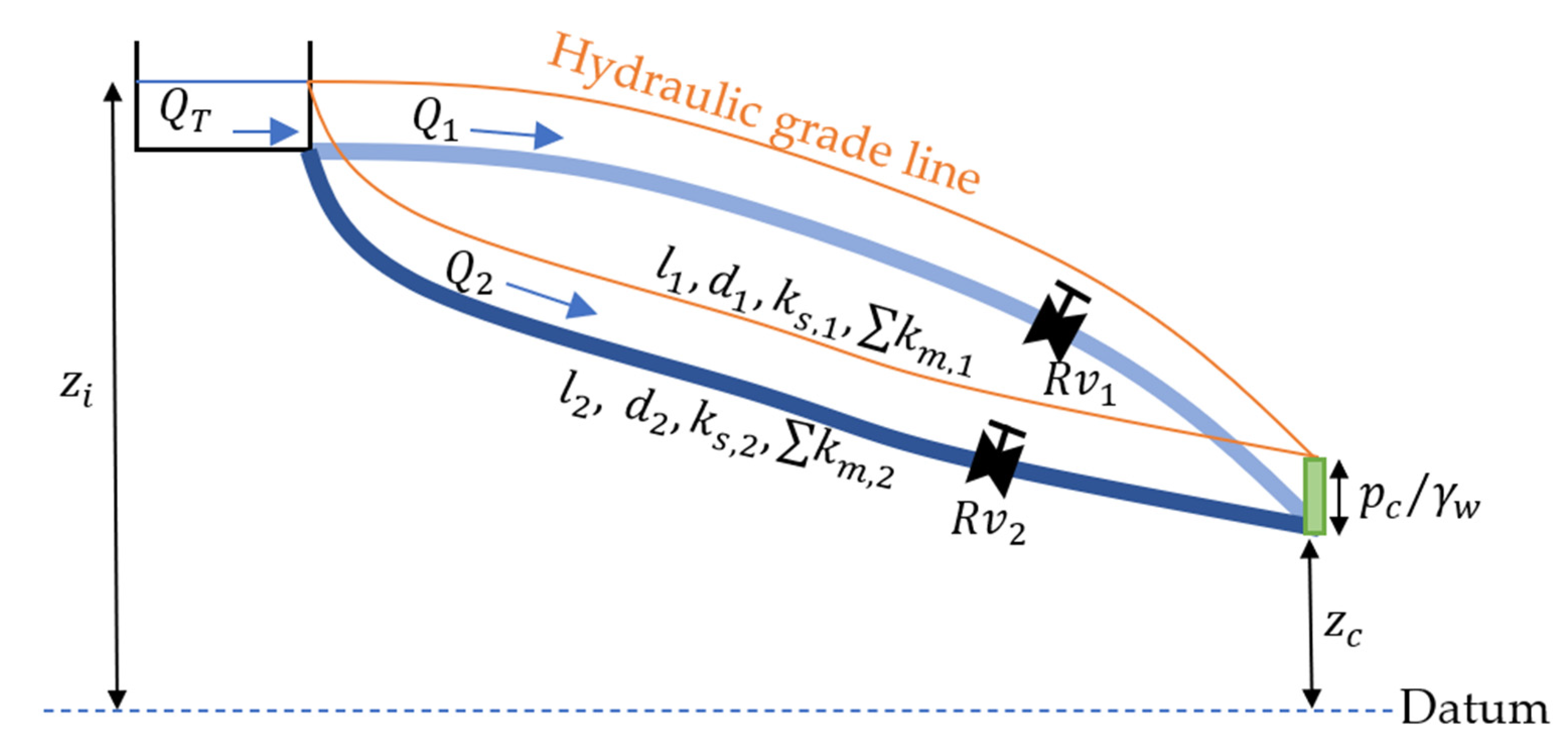
3.1. Application to the Case of Two Parallel Pipes

The case of two parallel ($n$ = 2) pipes is considered in this research, as shown in Figure 2. More complex installations can be analyzed with the mathematical model since this model is entirely general.

The corresponding formulations can be written as shown in

Table 2. Algebraic-differential equation system applied to the case of two parallel pipes.

Description	Formula	Equation No.
Mass oscillation equation applied to the first parallel pipe	$\frac{d{Q}_1}{dt}=\frac{\left[z_u-z_c-\raisebox{1ex}{$p_c$}\!\left/ \!\raisebox{-1ex}{${\gamma }_w$}\right.\right]g\pi d_1^2}{4l_1}-\frac{2f_1{Q}_1\left|Q_1\right|}{\pi d_1^3}-\frac{R_{v,1}{Q}_1\left|Q_1\right|g\pi d_1^2}{4l_1}-\frac{2\sum k_{m,1}{Q}_1\left|Q_1\right|}{\pi l_1{d}_1^2}$	(6)
Mass oscillation equation applied to the second parallel pipe	$\frac{d{Q}_2}{dt}=\frac{\left[z_u-z_c-\raisebox{1ex}{$p_c$}\!\left/ \!\raisebox{-1ex}{${\gamma }_w$}\right.\right]g\pi d_2^2}{4l_2}-\frac{2f_2{Q}_2\left|Q_2\right|}{\pi d_2^3}-\frac{R_{v,2}{Q}_2\left|Q_2\right|g\pi d_2^2}{4l_2}-\frac{2\sum k_{m,2}{Q}_2\left|Q_2\right|}{\pi l_2{d}_2^2}$	(7)
Continuity equation	$\frac{p_c}{{\gamma }_w}={\left(\frac{Q_1+Q_2-C_d\overline{Q_d}-C_i\overline{Q_i}-C_c\overline{Q_c}-C_o\overline{Q_o}}{K_{f,1}+K_{f,2}}\right)}^{\frac{1}{\beta }}$	(8)
Swamee–Jain equation applied to the first parallel pipe	$f_1=\frac{0.25}{{\left[\mathbf{log}\left(\frac{k_{s,1}}{3.7d_1}+\frac{5.74}{{\mathbf{R}\mathbf{e}}_1^{0.9}}\right)\right]}^2}$	(9)
Swamee–Jain equation applied to the second parallel pipe	$f_2=\frac{0.25}{{\left[\mathbf{log}\left(\frac{k_{s,2}}{3.7d_2}+\frac{5.74}{{\mathbf{R}\mathbf{e}}_2^{0.9}}\right)\right]}^2}$	(10)

.

This problem involves a set of five equations with initial conditions given as $Q_1\left(0\right)=Q_{\mathrm{1,0}}$ and $Q_2\left(0\right)=Q_{\mathrm{2,0}}$. It constitutes a well-posed problem, the solution of which describes the system’s behavior. $Q_{\mathrm{1,0}}$ and $Q_{\mathrm{2,0}}$ are computed through an extended period simulation. The objective is to calculate the five unknown variables: $Q_1,Q_2,f_1,f_2$, and $p_c/{\gamma }_w$. The system’s behavior is determined through the numerical resolution of Equations (6)–(10). The problem’s boundary conditions are defined by a reservoir located upstream and a regulating valve downstream, representing the classical boundary conditions.

3.2. Data

An analysis using an extended period simulation of a two-parallel pipes system revealed that the initial flow rate conditions were $Q_1\left(0\right)=$ 0.078 m³/s and $Q_2\left(0\right)=0.045$ m³/s, similar to the scheme depicted in Figure 2. The characteristics of the two parallel pipes are as follows: $d_1$= 250 mm, $l_1$= 1200 m, $d_2$= 200 mm, $l_2$= 1100 m, $\sum k_{m,1}=$ 3, $\sum k_{m,2}=$ 5, $R_{v,1}$ = 240 ms²/m⁶, $R_{v,2}$ = 190 ms²/m⁶, and $k_{s,1}=k_{s,2}=$0.0015 mm. The pipe elevation at the first node ($z_i$) is 35 m, while at the common node ($z_c$) it is 0 m. The mean values of water flow rate for domestic ($\overline{Q_d}$) and official consumption ($\overline{Q_o}$) are 65 and 22 L/s, respectively. A kinematic viscosity of 1 × 10⁻⁶ m/s² was considered for the analysis. The remaining consumption $Q_i$ and $Q_c$ are null in this application. Figure 3 shows consumption patterns for both domestic and official purposes throughout the first 180 s. The calibration process, conducted during an extended period simulation, yielded emitter coefficients of $K_{f,1}$ = 0.0085 m³/s/m^0.5 and $K_{f,2}$ = 0.0045 m³/s/m^0.5, with an exponent coefficient $\beta$ of 0.5. The regulating valve is initially opened, followed by a partial closure, and it ultimately returns to its initial position in terms of the percentage of opening. During this time, modulation coefficients of 0.3 and 0.4 are observed for domestic and official consumption, respectively.

4. Results

The numerical resolution of the five unknown variables ($Q_1$, $Q_2$, $\frac{p_c}{{\gamma }_w}$, $f_1$, and $f_2$) was accomplished by analyzing data from the two parallel pipes, as depicted in Figure 4. The simulation was conducted for the initial 180 s.

The analysis of these five variables was conducted. Figure 4a shows the water flow rate patterns for both pipes. The minimum value is 45.1 L/s (at 13.0 s) for pipe 1, while pipe 2 reaches a minimum value of 35.9 L/s (at 4.5 s). After $t$ = 45 s, both pipes exhibit nearly identical trends, with constant values of 60.6 L/s for pipe 1 and 37.5 L/s for pipe 2. However, the variable $Q_2$ displays some fluctuations over time, reaching a second peak value of 41.4 m at 30.0 s. The pressure head pulses at the common node are presented in Figure 4b. The initial pressure head value is 53.06 m. Rapidly, the partial closure of both regulating valves causes the pressure head to decrease to a minimum value of 17.41 m at 12.0 s. Subsequently, the pressure head increases and stabilizes at around 28.75 m (at 60.0 s). Figure 4c illustrates the friction factor for both parallel pipes, with values varying from 0.0137 to 0.0152 for pipe 1 and from 0.0146 to 0.0152 for pipe 2.

The total flow rate ($Q_T$) and flow rate of leaks ($Q_{Tl}$) were computed for the two parallel pipes. These two formulations are used to elucidate the extent of water volume leakage during transient events involving regulating valves. The results of these variables are illustrated in Figure 5. It becomes evident that a higher emitter coefficient corresponds to an increased water volume leakage, as exemplified by pipes 1 and 2. Furthermore, the total flow rate ($Q_1+Q_2$) exhibits a comparable pattern to the total flow rate of leaks ($Q_{Tl}$). The occurrences of maximum and minimum water flow coincide with the extreme values of water leakages. For example, the minimum values for both total water flow and water flow from leaks are 82.54 L/s and 52.24 L/s, respectively, occurring at $t=$12.0 s. For the initial 180 s, the injected water volume to the system is 17.46 m³, while the water leakage volume is 12.35 m³.

Finally, a comparison was conducted between a single pipe installation and the parallel installations under analysis, as illustrated in Figure 6. The characteristics of the single pipe match those of Pipe 1 in the parallel system. It was observed that higher pressure head values at the end of the system were achieved with an increased number of parallel pipes. Consequently, the parallel pipe configuration led to a greater quantity of water leakages when compared to a single installation. In this analysis, the total water leakage during the first 180 s in the single pipe amounted to 7.57 m³, which was lower than the value obtained in the parallel system (12.35 m³).

5. Discussion

The proposed model is well-suited for assessing transient events occurring within a timeframe, given its consideration of system inertia [23]. The term $dQ/dt$ is employed to account for valve maneuvers. Utilities typically utilize extended period simulation to implement strategies for addressing water leakages in water distribution systems [9]. This is crucial as it enables more accurate computation.

Detecting leaks in water distribution systems poses a challenge for water utilities. Nevertheless, once leaks have been identified, the proposed model can be employed to assess water volume losses under various valve maneuver scenarios. Neither the extended period simulation (which serves as the current leak prediction model) [16] nor the proposed model (which incorporates system inertia for enhanced accuracy) can pinpoint the exact locations of leaks.

The PDE system, or elastic model equations, represents the more intricate formulations for transient events, entailing the analysis of water and pipe elasticity. However, suppose water cannot compress or expand during a transient event or the pipe cannot deform its thickness. In that case, system inertia can be examined using a rigid column approach, as proposed by our model [29]. Leaks operate similarly to water-release orifices; consequently, they reduce head pressure.

A mathematical model for the accurate determination of water volume leakages in all parallel pipe systems, which is based on the mass oscillation equation (rigid water column model), has been presented in this research. It signifies a novel advancement in the current literature, as no governing equations have been previously documented for modeling this situation. The proposed model permits the computation of water leakages even when regulating valves are acting, which implies that the system inertia is considered in calculations. In this sense, the mathematical model is more robust than the extended period simulation in this scenario. The mathematical model is presented in a general way and can be used to analyze parallel pipe systems. The numerical resolution includes the mass oscillation equation to know the behavior of water movement, the analysis of pressure-head-dependent and pressure-head-independent consumption, and the friction factor computation.

Based on the results of the practical application, some remarks can be drawn:

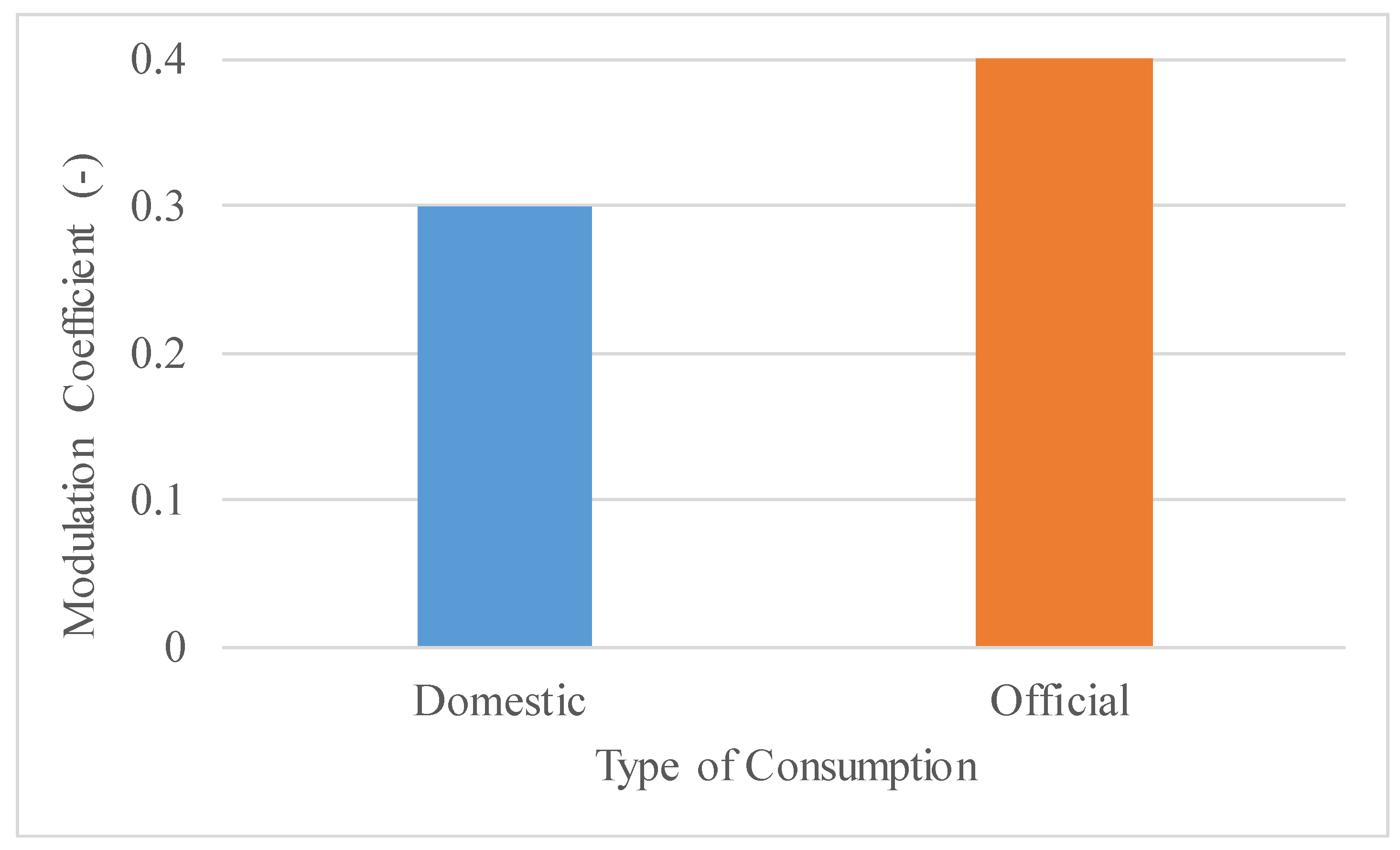
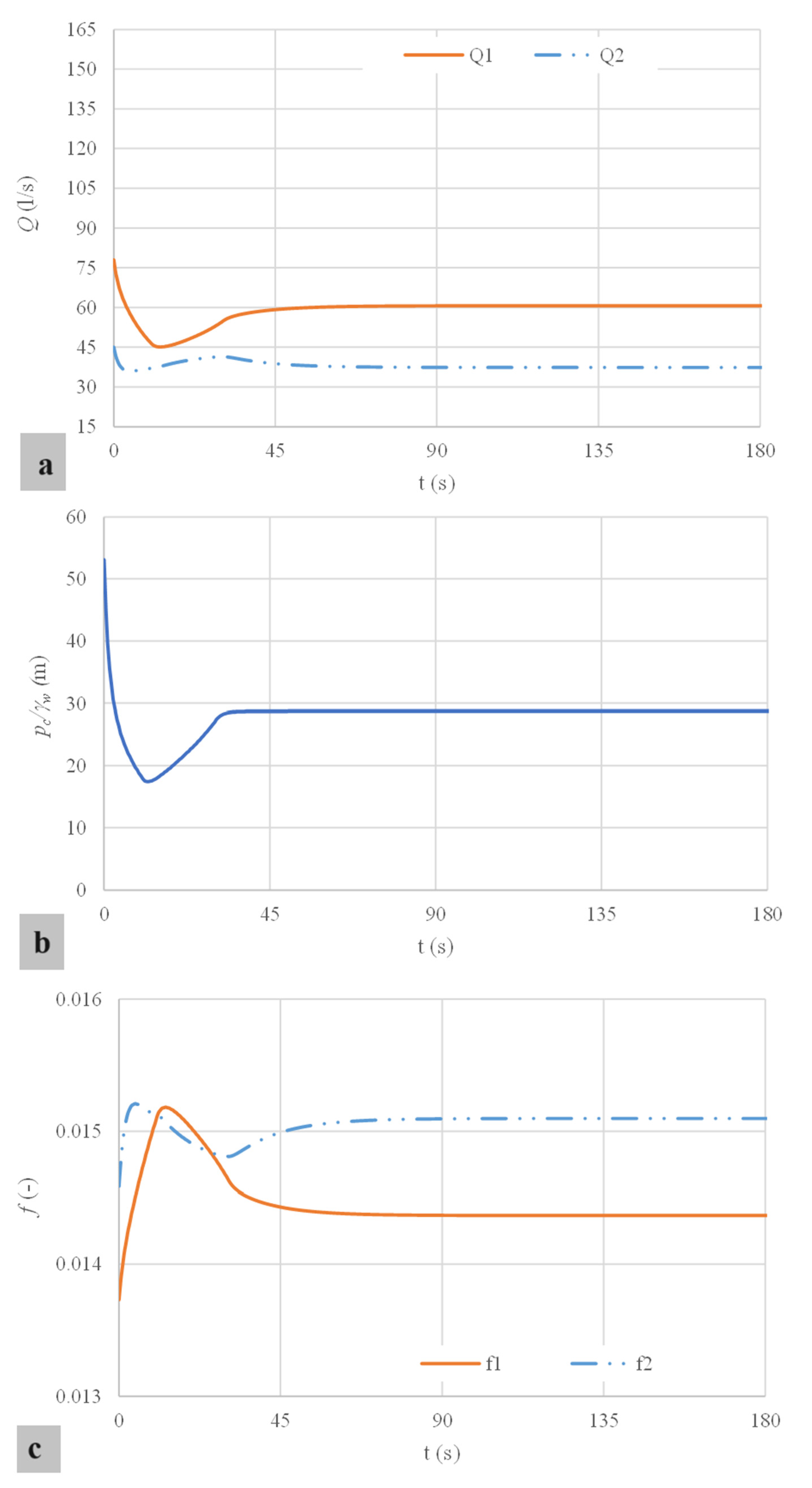
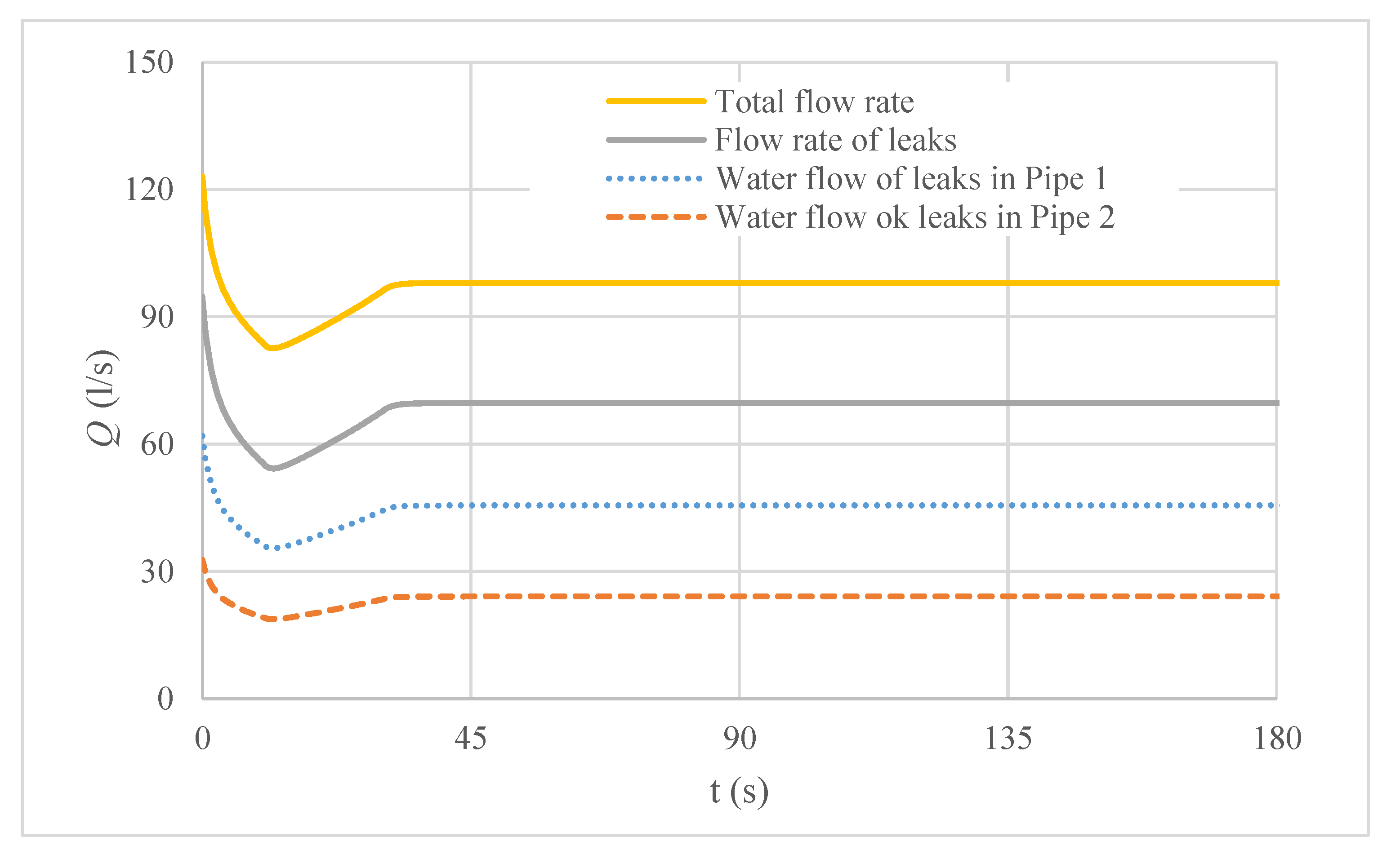
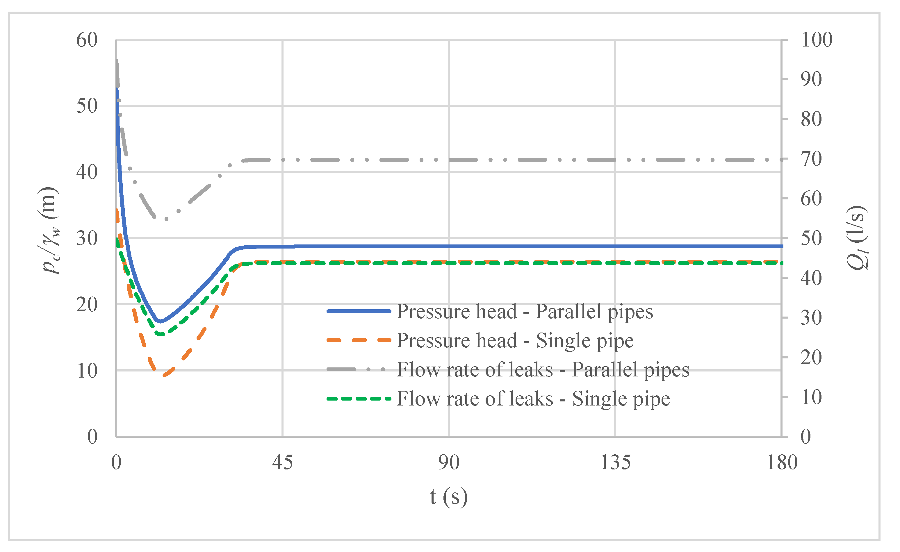
• The practical application is composed of two parallel pipes, and its results can be used for engineers and designers to compute the total leakage volume when two regulating valves are operated following different maneuvers. The mathematical model shows that each problem of parallel pipe requires $2i+1$ equations to be solved. In this case ($i=2$), the variables to compute are $Q_1$, $Q_2$, $\frac{p_c}{{\gamma }_w}$, $f_1$, and $f_2$. Due to the regulating valves acting, the pressure head patterns are changing even for constant consumption (domestic and official), ranging from 53.06 m to 28.75 m. The two parallel pipes’ water flow and friction factor patterns are different and should be separately computed.
• When more parallel pipes are added to reinforce a line, the amount of water volume of leakages is increased since, during the operational time, water installations have more orifices along their length, provoking more water losses. It is then of the utmost importance to reduce the number of parallel pipes during the design stage to save energy production in the injected water flow.

The primary limitation of the proposed model is that it has not been specifically designed for complex installations. The current research serves as an initial phase, laying the groundwork for extending this methodology to more intricate networks. Additionally, it is noteworthy that the numerical resolution of the proposed model is more intricate compared to the extended period simulation, resulting in a longer computational time.

In summary, the proposed model can calculate water leaks in much greater detail than the quasi-static models that are usually used. Thus, the rigid inertial model is suitable for detecting rapid flow variations (for example, rapid regulating valve maneuvers) with greater precision.

References

1. Lambert, A.; Hirner, W. Losses from Water Supply Systems: A Standard Terminology and Recommended Performance Measures; IWA: London, UK, 2000. [Google Scholar]
2. Lambert, A.O.; Brown, T.G.; Takizawa, M.; Weimer, D. A review of performance indicators for real losses from water supply systems. J. Water Supply Res. Technol. AQUA 1999, 48, 227–237. [Google Scholar] [CrossRef]
3. IBNET. IBNET Indicator Heat Map. February 2021. Available online: https://database.ib-net.org/Reports/Indicators/HeatMap (accessed on 1 February 2024).
4. United Nations. Sustainable Development Goals. Available online: https://sdgs.un.org/goals (accessed on 1 February 2024).
5. Bibri, S.E.; Krogstie, J. Smart sustainable cities of the future: An extensive interdisciplinary literature review. Sustain. Cities Soc. 2017, 31, 183–212. [Google Scholar] [CrossRef]
6. Ishiwatari, Y.; Mishima, I.; Utsuno, N.; Fujita, M. Diagnosis of the ageing of water pipe systems by water quality and structure of iron corrosion in supplied water. Water Sci. Technol. Water Supply 2013, 13, 178–183. [Google Scholar] [CrossRef]
7. Li, R.; Huang, H.; Xin, K.; Tao, T. A review of methods for burst/leakage detection and location in water distribution systems. Water Sci. Technol. Water Supply 2015, 15, 429–441. [Google Scholar] [CrossRef]
8. Cimorelli, L.; D’Aniello, A.; Cozzolino, L.; Pianese, D. Leakage reduction in WDNs through optimal setting of PATs with a derivative-free optimizer. J. Hydroinform. 2020, 22, 713–724. [Google Scholar] [CrossRef]
9. Ramos, H.M.; Kuriqi, A.; Besharat, M.; Creaco, E.; Tasca, E.; Coronado-Hernández, O.E.; Pienika, R.; Iglesias-Rey, P. SmartWater Grids and Digital Twin for the Management of System Efficiency in Water Distribution Networks. Water 2023, 15, 1129. [Google Scholar] [CrossRef]
10. Alzamora, F.M.; Carot, M.H.; Carles, J.; Campos, A. Development and Use of a Digital Twin for the Water Supply and Distribution Network of Valencia (Spain). In Proceedings of the 17th International Computing & Control for the Water Industry Conference, Exeter, UK, 1–4 September 2019. [Google Scholar]
11. Jiang, Z.; Guo, Y.; Wang, Z. Digital Twin to Improve the virtual-real Integration of Industrial Iot. J. Ind. Inf. Integr. 2021, 22, 100196. [Google Scholar] [CrossRef]
12. Liu, M.; Fang, S.; Dong, H.; Xu, C. Review of Digital Twin about Concepts, Technologies, and Industrial Applications. J. Manuf. Syst. 2021, 58, 346–361. [Google Scholar] [CrossRef]
13. Niu, W.J.; Feng, Z.K. Evaluating the performances of several artificial intelligence methods in forecasting daily streamflow time series for sustainable water resources management. Sustain. Cities Soc. 2021, 64, 102562. [Google Scholar] [CrossRef]
14. Lu, Q.; Parlikad, A.K.; Woodall, P.; Don Ranasinghe, G.; Xie, X.; Liang, Z.; Konstantinou, E.; Heaton, J.; Schooling, J. Developing a Digital Twin at Building and City Levels: Case Study of West Cambridge Campus. J. Manag. Eng. 2020, 36, 05020004. [Google Scholar] [CrossRef]
15. Asadi, S.; Nazari-Heris, M.; Rezaei Nasab, S.; Torabi, H.; Sharifironizi, M. An Updated Review on Net-Zero Energy and Water Buildings: Design and Operation. In Food-Energy-Water Nexus Resilience and Sustainable Development: Decision-Making Methods, Planning, and Trade-Off Analysis; Springer: Cham, Switzerland, 2020; pp. 267–290. [Google Scholar]
16. Ávila, C.; Sánchez-Romero, F.-J.; López-Jiménez, P.A.; Pérez- Sánchez, M. Improve Leakage Management to Reach Sustainable Water Supply Networks through by Green Energy Systems. Optimized Case Study. Sustain. Cities Soc. 2022, 83, 103994. [Google Scholar] [CrossRef]
17. Jowitt, P.W.; Xu, C. Optimal valve control in water-distribution networks. J. Water Resour. Plan. Manag. 1990, 116, 455–472. [Google Scholar] [CrossRef]
18. Giustolisi, O.; Savic, D.; Kapelan, Z. Pressure-driven demand and leakage simulation for water distribution networks. J. Hydraul. Eng. 2008, 134, 626–635. [Google Scholar] [CrossRef]
19. Al-Washali, T.; Sharma, S.; Kennedy, M. Methods of assessment of water losses in water supply systems: A review. Water Resour. Manag. 2016, 30, 4985–5001. [Google Scholar] [CrossRef]
20. Samir, N.; Kansoh, R.; Elbarki, W.; Fleifle, A. Pressure control for minimizing leakage in water distribution systems. Alex. Eng. J. 2017, 56, 601–612. [Google Scholar] [CrossRef]
21. Schwaller, J.; Van Zyl, J.V. Modeling the pressure-leakage response of water distribution systems based on individual leak behavior. J. Hydraul. Eng. 2015, 141, 04014089. [Google Scholar] [CrossRef]
22. Coronado-Hernández, O.E.; Pérez-Sánchez, M.; Arrieta-Pastrana, A.; Fuertes-Miquel, V.S.; Coronado-Hernández, J.R.; Quiñones-Bolaños, E.; Ramos, H.M. Dynamic effects of a regulating valve in the assessment of water leakages in single pipelines. Water Resour. Manag. 2024. [Google Scholar] [CrossRef]
23. Fuertes-Miquel, V.S.; Coronado-Hernández, O.E.; Mora-Meliá, D.; Iglesias-Rey, P.L. Hydraulic modeling during filling and emptying processes in pressurized pipelines: A literature review. Urban Water J. 2019, 16, 299–311. [Google Scholar] [CrossRef]
24. Coronado-Hernández, O.E.; Fuertes-Miquel, V.S.; Iglesias-Rey, P.L.; Martínez-Solano, F.J. Rigid water column for simulating the emptying process in a pipeline using pressurized air. J. Hydraul. Eng. 2018, 144, 06018004. [Google Scholar] [CrossRef]
25. Prest, E.I.; Schaap, P.G.; Besmer, M.D.; Hammes, F. Dynamic Hydraulics in a Drinking Water Distribution System Influence Suspended Particles and Turbidity, but Not Microbiology. Water 2021, 13, 109. [Google Scholar] [CrossRef]
26. Tsagkari, E.; Connelly, S.; Liu, Z.; McBride, A.; Sloan, W.T. The role of shear dynamics in biofilm formation. npj Biofilms Microbiomes 2022, 8, 33. [Google Scholar] [CrossRef] [PubMed]
27. Eshkabilov, S.L. Practical MATLAB Modeling with Simulink: Programming and Simulating Ordinary and Partial Differential Equations; Apress: Berkeley, CA, USA, 2020. [Google Scholar]
28. Altowayti, W.A.H.; Othman, N.; Tajarudin, H.A.; Al-Dhaqm, A.; Asharuddin, S.M.; Al-Gheethi, A.; Alshalif, A.F.; Salem, A.A.; Din, M.F.M.; Fitriani, N.; et al. Evaluating the Pressure and Loss Behavior in Water Pipes Using Smart Mathematical Modelling. Water 2021, 13, 3500. [Google Scholar] [CrossRef]
29. Abreu, J.; Cabrera, E.; Izquierdo, J.; García-Serra, J. Flow Modeling in Pressurized Systmes Revisited. J. Hydraul. Eng. 1999, 125, 1154–1169. [Google Scholar] [CrossRef]
Figure 1. Plan view illustrating a general schematic of n parallel pipes.
Water 16 00926 g001
Figure 2. Scheme for two parallel pipes.
Water 16 00926 g002
Figure 3. Domestic and official consumption patterns for the first 180 s.
Water 16 00926 g003
Figure 4. Results of main variables: (a) water flow rate; (b) pressure head; (c) friction factor.
Water 16 00926 g004
Figure 5. Analysis of water flow and leakages in parallel pipes.
Water 16 00926 g005
Figure 6. Comparison between single and parallel systems.
Water 16 00926 g006