Development of Pipeline Transient Mixed Flow Model with Smoothed Particle Hydrodynamics Based on Preissmann Slot Method

Abstract

The accurate modeling and understanding of complex transient mixed pipe flows is crucial for the optimal design and safe and efficient operation in pipeline systems such as urban drainage systems. Currently, the predominant approach for modeling free-surface-pressurized flows relies on grid-based numerical schemes, with comparatively limited capability for exploring its complex phenomena. This study proposed a novel one-dimensional numerical model that integrates the smoothed particle hydrodynamics (SPH) method with the Preissmann slot method (PSM) to explore transient mixed flows in pipeline systems, with better potential capability for exploring more mixed flow phenomena. Empirical parameters of the proposed SPH-PSM model were optimized for improving the numerical accuracy and stability, and the applicable range for these empirical parameters was recommended. The performances of the proposed model were evaluated by different flow regimes, including one free surface case, one fully pressurized case, and two transient mixed-flow cases. The simulation results of different flow regimes demonstrated a high level of agreement with the reference data, indicating the good capability of the SPH-PSM model in simulating complex flow regimes in pipeline systems. Therefore, the proposed SPH-PSM model can be an alternative way for modeling, exploring, and understanding the complex transient mixed flows in pipeline systems.

1. Introduction

The transient mixed flow is a complicated phenomenon that involves a combination of free surface and pressurized flow regimes. This phenomenon can result in significant damage to the pipeline infrastructure and connected equipment, leading to hydraulic failures in urban drainage systems (UDSs), such as blown-off manhole covers, geysers, and pipe bursts, due to high positive and negative pressure surge fluctuations. Laboratory experiments have been conducted to improve the understanding of the complex flow dynamics involving transition regimes and instability [1,2,3]. Furthermore, numerical analysis models of transient mixed flow, such as the mouse, hydro-works, and the storm water management model (SWMM) [4,5,6], were developed to improve the design and operation process in UDSs. However, as pointed out by Bousso et al. [7], the existing numerical models for transient mixed flow have limitations due to the characteristics of multiple phases, transition regimes, and dynamic instabilities (e.g., flow instability, dry bed instability, roll wave instability, free-surface-pressurized flow instability, etc.). Therefore, developing an accurate transient mixed-flow model for UDSs remains a challenging task.

Currently, the one-dimensional numerical model of transient mixed flow in pipes can be categorized into single-phase and two-phase [8]. Single-phase models such as the Preissmann slot method (PSM) and the two-component pressure approach (TPA) model employ one single equation for both free surface and pressurized flows [3,9]. This class of model relaxed the incompressibility to allow additional mass storage. To simulate the negative pressure using PSM, Kerger et al. [10] introduced an original negative PSM model for simulating sub-atmospheric pressurized flow. The advantages of the single-phase models are computational efficiency, simplicity, and unified equations. However, the use of large pressure wave celerity can lead to numerical oscillations at the interface during transitions, and the model’s scalability is limited (e.g., in the two-phase flow of water and gas).

Contrary to single-phase models, a two-phase coupled model explicitly considers the gas phase, mainly by the rigid column approach [11], finite-volume strategy [12,13], or fully in the four equations model [14]. Two-phase models incorporate additional equations to describe gas phase and different regimes, allowing for a more comprehensive exploration of the interactions between air and water in mixed flows [1]. And two-phase models could use larger pressure wave celerity in the simulation. However, the implementation of two-phase coupled model requires more complex solving and computational resources [7]; additionally, the code implementation of the model is more complex.

Therefore, considering the practicality of the model, this paper adopted the simple and easily implementable single-equation approach. PSM is a representative transient mixed-flow model and its simulation results are accurate and reliable, with well-established applications in numerous cases. In the latest SWMM5.2 model, PSM was also employed as the transient mixed-flow simulation method [15].

In terms of numerical methods, the traditional numerical schemes used for models described above generally fall into three categories: finite volume method (FVM) [16,17], method of characteristics (MOC) [1,18], and finite difference method (FDM) [2,9]. However, these mesh-based numerical methods still encounter challenges in multiphase transition interface tracking and irregular geometry boundary treatment [7]. On the contrary, the mesh-free methods, such as particle in cell (PIC), smoothed particle hydrodynamics (SPH), etc., have demonstrated significant advantages in dealing with the above-mentioned issues due to their advanced mesh-free features [19]. As a typical mesh-free Lagrangian method, SPH has been rapidly developed due to its excellent potential in modeling fluid dynamics problems characterized by violently changing boundaries or interfaces, complex geometries, and flexibility in tracing moving boundaries. For example, SPH is widely used for modeling dam breaks, sea waves, underwater explosions, and pipe or channel flow modeling [20,21,22]. For the pipe or channel flow modeling, most SPH studies were developed to solve the open-channel flow [23,24,25] and the pressurized flow [26,27]. Nevertheless, there is a scarcity of research concerning the application of the SPH method for modeling the transient mixed flow in pipelines [28,29]. Furthermore, mixed flow phenomena are characterized by a dynamic transition interface within a closed conduit, while the SPH method has been proven effective in capturing discrete processes and tracking moving boundaries in transient flows, such as column separation and rapid filling [28]. Therefore, exploring the feasibility and significance of applying the SPH method to solve 1D mixed flow models becomes imperative.

In conclusion, despite the advancements in numerical analysis models for transient mixed flow, the existing numerical models have inadequacies due to their simplicity or the constraints of mesh-based methods. Consequently, the objective of this study is to develop a new numerical solution for modeling transient mixed-flow pipeline systems using the SPH method. Coupled with the PSM model, a SPH-PSM model was proposed and evaluated, focusing on exploring the advanced mesh-free features of SPH in capturing and tracking complex interfaces for pipeline transient mixed flow. The key contributions of this work can be summarized as follows: (1) the development of formulas for the PSM model based on the SPH method; (2) the exploration and optimization of various related parameters; (3) the testing and validation of different flow regimes, including free surface, fully pressurized, and transition mixed flow in pipelines.

2. Numerical Methods

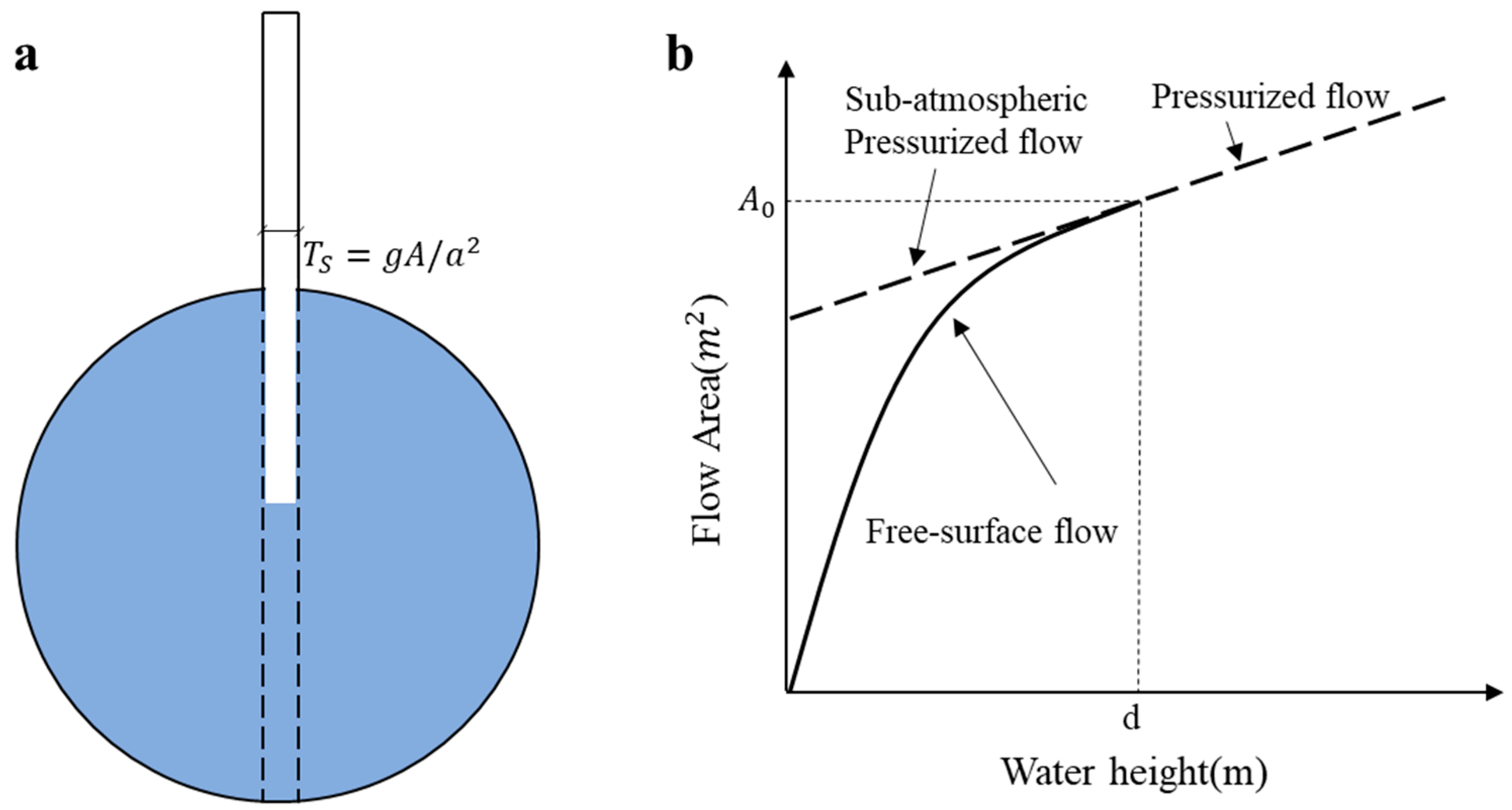
2.1. The Preissmann Slot Model

For a one-dimensional open channel flow, the system of flow governing equations can be written as:

$$\begin{array}{c}\left\{\begin{array}{c}\frac{dA}{dt}=-A\frac{\partial \left(v\right)}{\partial x}\\ \frac{dQ}{dt}=-Q\frac{\partial \left(v\right)}{\partial x}-g\frac{\partial I}{\partial x}+gA\left(S_0-S_f\right)\end{array}\right.\end{array}$$

(1)

where $A$ is the flow area; $Q$ is the flow discharge rate; $v$ is the velocity vector; $S_0$ = $-d{z}_b∕dx$ is the bottom slope ($z_b$ is the bottom elevation); and $S_f$ is the friction slope, which is evaluated here according to the Manning formula. The hydrostatic pressure term $I$ is defined as $I={\int }_0^h\left(h-\eta \right)\sigma (h,\eta )d\eta$, where $h$ is the water depth and $\sigma (h,\eta )$ is the cross-sectional width at an elevation $\eta$ above the bottom.

According to the Preissmann slot model [30], pressurized flow can equally be calculated through the Saint-Venant equations by adding a conceptual narrow slot on the top of a closed conduit (Figure 1a). When the water level is above the conduit crown, it provides a conceptual free-surface flow, and the slot width $T_s$ should be set according to the relation:

$$\begin{array}{c}{T}_s=\frac{gA}{a^2}\end{array}$$

(2)

where $a$ is the pressure wave celerity.

To overcome the limitation of the original PSM model in simulating negative pressure, this study adopts the negative narrow slot proposed by Kerger et al. [10]. This approach extends the narrow slot in a straight line below the top of the pipe (Figure 1). The water level below the pipe crown represents two flow area values, one for the free surface flow area and another for the negative pressure flow area. The selection of the appropriate flow area depends on the ventilation conditions.

In the case of a pipe with a circular cross-section, the relevant cross-sectional area can be expressed as follows:

$$\begin{array}{c}A=\left\{\begin{array}{cc}{A}_c+h_s{T}_s& \mathrm{Pressurized}\mathrm{flow}\\ A_c-h_s{T}_s& \mathrm{Sub-atomspheric}\mathrm{pressurized}\mathrm{flow}\\ \frac{D^2\left(\theta -\mathrm{s}\mathrm{i}\mathrm{n}\theta \right)}{8}& \mathrm{Free-surface}\mathrm{flow}\end{array}\right.\end{array}$$

(3)

where $A_C$ is the cross−sectional area of a circular pipe; $h_S$ is the additional head of the pipe; and $\theta$ is the angle between the free surface and the center of the pipe.

2.2. Smoothed Particle Hydrodynamics Method

The SPH method is a complete Lagrangian meshless method, where the entire system is represented by the number of particles with independent masses. The construction of the SPH equation involves two key steps: kernel approximation and particle approximation. Based on this method, the physical property of particle $i$ can be discretized by the following function [31]:

$$\begin{array}{c}\begin{array}{c}f\left(x_i\right)={\int }_{\mathsf{\Omega }}f\left(x^{\prime }\right)W\left(x_i-x^{\prime },h\right)d{x}^{\prime }\approx {\displaystyle \sum _i}f\left(x_j\right)W\left(x_i-x_j,h\right)\frac{m_j}{A_j}\\ \nabla f\left({\mathrm{x}}_i\right)={\int }_{\mathsf{\Omega }}f\left({\mathrm{x}}^{\prime }\right)\nabla W\left({\mathrm{x}}_i-{\mathrm{x}}^{\prime },h\right)d{\mathrm{x}}^{\prime }\approx {\displaystyle \sum _i}\left(f\left({\mathrm{x}}_j\right)-f\left({\mathrm{x}}_i\right)\right)\nabla W\left({\mathrm{x}}_i-{\mathrm{x}}_j,h\right)\frac{m_j}{A_j}\end{array}\end{array}$$

(4)

where $W\left({\mathit{x}}_{\mathit{i}}-{\mathit{x}}^{\prime },h\right)$ is the kernel function; h is the smoothing length, which determines support domain Ω; $m_j$ is the mass of particle $j$; $A_j$ is the flow area of particle $j$; and ${\mathit{x}}_{\mathit{j}}$ is the position of particle $j$.

Although the SPH method has been widely applied in various fields, the traditional SPH method suffers from the boundary defect caused by the truncation of kernel support near the boundaries. To address this drawback, this study employs the corrective SPH (CSPH) method based on Taylor expansion for correction [32,33]. The corrected kernel approximation and gradient are derived as follows:

$$\begin{array}{c}\begin{array}{c}\widetilde{W_{ij}}=\frac{W_{ij}}{\sum _{j=1}^N\frac{m_j}{A_j}{W}_{ij}}\\ \widetilde{{\nabla }_i{W}_{ij}}=\frac{{\nabla }_i{W}_{ij}}{\sum _{j=1}^N\frac{m_j}{A_j}\left(x_j-x_i\right)·{\nabla }_i{W}_{ij}}\end{array}\end{array}$$

(5)

where $\widetilde{W_{ij}}$ is the corrected kernel function of $W_{ij}$; and $\widetilde{{\nabla }_i{W}_{ij}}$ is the first-order corrected gradient of kernel function ${\nabla }_i{W}_{ij}$.

2.3. Discretization of the PSM with SPH

After the aforementioned modifications, the discretized form of PSM, referred to as SPH-PSM, can be approximated as follows:

$$\begin{array}{c}\left\{\begin{array}{c}\frac{D{A}_i}{Dt}=-{\displaystyle \sum _j}{m}_j\left(\frac{Q_j}{A_j}-\frac{Q_i}{A_i}\right)·\widetilde{\nabla W_{ij}}+L_i\\ \begin{array}{c}\frac{D{Q}_i}{Dt}=-\frac{Q_i}{A_i}{\displaystyle \sum _j}{m}_j\left(\frac{Q_j}{A_j}-\frac{Q_i}{A_i}\right)·\widetilde{\nabla W_{ij}}-{gA}_i{\displaystyle \sum _j}{m}_j\left(\frac{I_j}{{A_j}^2}+\frac{I_i}{{A_i}^2}\right)·\widetilde{\nabla W_{ij}}\\ +{\displaystyle \sum _j}\frac{m_j}{A_j}{\Pi }_{ij}·\widetilde{\nabla W_{ij}}+g{A}_i\left(S_{0,i}-S_{f,i}\right)\end{array}\end{array}\right.\end{array}$$

(6)

The PSM model uses a detailed integral expression to express $I$, which is simplified as Equation (7), assuming the pipe is circular.

$$\begin{array}{c}I=\left\{\begin{array}{ll}g{A}_c\left(\frac{D}{2}+h_s\right)+g{T}_s{h}_s^2/2& \mathrm{Pressurized}\mathrm{flow}\\ g{A}_c\left(\frac{D}{2}{-h}_s\right)+g{T}_s{h}_s^2/2& \mathrm{Sub-atomspheric}\mathrm{pressurized}\mathrm{flow}\\ \frac{1}{24}g{D}^3\left[3\mathrm{s}\mathrm{i}\mathrm{n}\left(\frac{\theta }{2}\right){\mathrm{s}\mathrm{i}\mathrm{n}}^3\left(\frac{\theta }{2}\right)3\left(\frac{\theta }{2}\right)\mathrm{c}\mathrm{o}\mathrm{s}\left(\frac{\theta }{2}\right)\right]& \mathrm{Free-surfage}\mathrm{flow}\end{array}\right.\end{array}$$

(7)

The kernel function should have properties such as compact support, normalization, symmetry, and smoothness. Currently, commonly used kernel functions include Gaussian [34], B-spline [35], and quintic-spline kernel functions [36]. The selection of the kernel function in this study will be determined through the model parameter tests in Section 3.1.

To reduce spurious numerical oscillations, the momentum equation is augmented with the normalized artificial viscosity term proposed by Ata et al. [37], which is more suitable for the SPH-SVEs model:

$$\begin{array}{c}{\mathsf{\Pi }}_{ij}=-A_{ij}\frac{{\lambda }_{ij}{(v}_i-v_j){(x}_i-x_j)}{\sqrt{{{(x}_i-x_j)}^2+{\epsilon }^2}}\end{array}$$

(8)

where $A_{ij}=(A_i+A_j)/2$; ${\lambda }_{ij}={(a}_i+a_j)\frac{1}{2};$ and $\epsilon$ is a small constant (chosen as 10⁻⁶), to avoid division by zero problem during the computations.

To improve the particle pressure distribution in the SPH method, a density diffusion term is introduced into the continuity equation [38]:

$$\begin{array}{c}{L}_i={\displaystyle \sum _{j=1}^N}\frac{m_j}{A_j}\gamma h_{ij}{\lambda }_{ij}\left(A_i-A_j\right)\frac{{(x}_i-x_j)}{{{(x}_i-x_j)}^2+{\epsilon }^2}\widetilde{{\nabla }_i{W}_{ij}}\end{array}$$

(9)

where $\gamma$ is the density diffusion coefficient; and $h_{ij}=0.5(h_i+h_i)$ is the average smoothing length of the particles.

2.4. Time Integration Scheme

In the SPH method, several time integration methods are commonly used, including the Euler method, leapfrog method [39], and second-order Runge–Kutta (RK2) method [40]. The effects of different time integration methods on the SPH-PSM will be analyzed in Section 3.1. The commonly used Euler method formula is as follows:

$$\begin{array}{c}{\mathit{U}}^{\left(n\right)}={\mathit{U}}^{\left(n-1\right)}+\mathcal{F}\left(t^{\left(n-1\right)},{\mathit{U}}^{\left(n-1\right)}\right)·∆t_{n-1}\end{array}$$

(10)

where $\mathit{U}$ is the conserved variable in the control equation; $\mathcal{F}$ is an expression for the particle approximation of the SPH method; $n$ is the computational step; and $∆t_n$ is the time step at the $n$.

Additionally, the time step size is set to satisfy the CFL condition:

$$\begin{array}{c}∆t\le \zeta ·\min \left(\frac{∆x_0}{a_i+{|v}_i|}\right)\end{array}$$

(11)

where ζ is the Courant number; $∆x_0$represents the initial spacing between particles; $a_i$denotes the pressure wave celerity of particle$i;$ and $v_i$ represents the flow velocity of particle $i$.

2.5. Boundary Treatments

Accurate and stable modeling relies on the proper treatment of complex boundary conditions. The boundary in SPH methods can be broadly classified into solid wall boundaries and open boundaries.

For solid wall boundaries, a commonly employed method involves introducing mirrored particles [41] to represent the boundaries. For open boundaries, the parameters of buffer particles are determined by the method of characteristics in combination with the energy conservation equation [23,42].

3. Test Results and Discussions

This section shows the impact of the SPH-PSM model parameters on accuracy, stability, and computational efficiency by idealized test cases with exact numerical solutions. Additionally, standard numerical cases and laboratory cases covering three flow regimes (open channel flow, pressurized flow, and transient mixed flow) were utilized to validate the accuracy and versatility of the SPH-PSM model. The simulation codes presented in this section were executed on a computer equipped with an AMD R7 8845H chip and 16 GB of RAM.

3.1. SPH-PSM Model Parameter Optimization

The parameters in the SPH-PSM model can be broadly categorized into two main types: (1) SPH-related parameters: initial particle number $n$, smoothing length $h$, kernel function $W\left(\mathit{x}-{\mathit{x}}^{\prime },h\right)$, density diffusion coefficient $\gamma$, time integration scheme, and Courant number $\zeta$; (2) PSM-related parameters: slot width $T_s$ and the pressure wave celerity $a$.

The discussion of model parameters is based on idealized test cases conducted in a square horizontal pipe with a length of 500 m and dimensions of $1\mathrm{m}\times 1\mathrm{m}$ from Dazzi et al. [43]. The initial discontinuity is located at $x=250\mathrm{m}$. The test scenario is illustrated in Figure 2. The $h_l$ and $v_l$ represent the piezometric head and flow velocity on the left side, while $h_r$ and $v_r$ represent those variables on the right side. Pipe friction is not considered here. The initial parameters for the three numerical experimental tests are shown in

Table 1. The initial conditions of the idealized tests from Dazzi et al. [43].

Test Case	${\mathit{h}}_{\mathit{l}}$ (m)	${\mathit{v}}_{\mathit{l}}$ (m/s)	${\mathit{h}}_{\mathit{r}}$ (m)	${\mathit{v}}_{\mathit{r}}$ (m/s)	Study Parameter
T1	3.0	0	0.5	0	SPH-related
T2	1.8	0.9	0.8	−1.0	SPH-related
T3	0.8	2.0	0.8	−2.0	PSM-related

.

The accuracy of the SPH-PSM model was evaluated by the $L_2$ norm formula. The reference data are from the numerical simulation results based on the exact Riemann solver proposed by Kerger et al. [17].

$$\begin{array}{c}{L}_2\left(\phi \right)=\sqrt{\frac{\sum _{i=1}^N{\left({\phi }_i^{SPH-PSM}-{\phi }_i^{REF}\right)}^2}{\sum _{i=1}^N{\left({\phi }_i^{REF}\right)}^2}}\end{array}$$

(12)

where the ${\phi }_i^{SPH-PSM}$ and ${\phi }_i^{REF}$ mean the value of the simulated results and reference data.

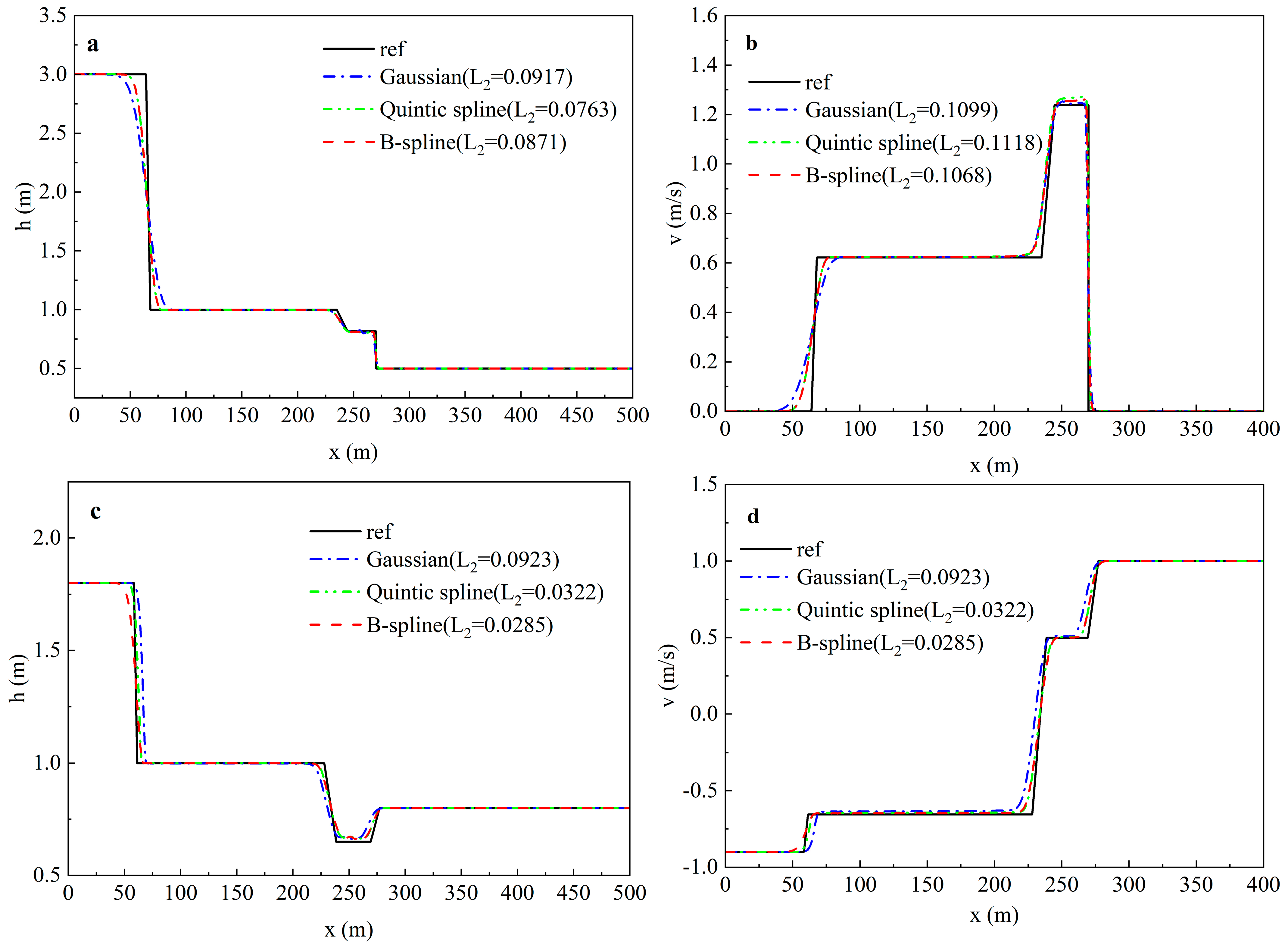
3.1.1. SPH-Related Parameters

The discussion of SPH-related parameters is based on Tests T1 and T2. For reference, a baseline configuration is used with the following settings: a particle number of 500, a smoothing length of 1.3$∆x_0$, B-spline as the kernel function, the density diffusion coefficient of 0.3, Euler integration as the time integration scheme, a Courant number of 0.5, and the pressure wave celerity is 30 m/s represented by a red dashed line in the figures.

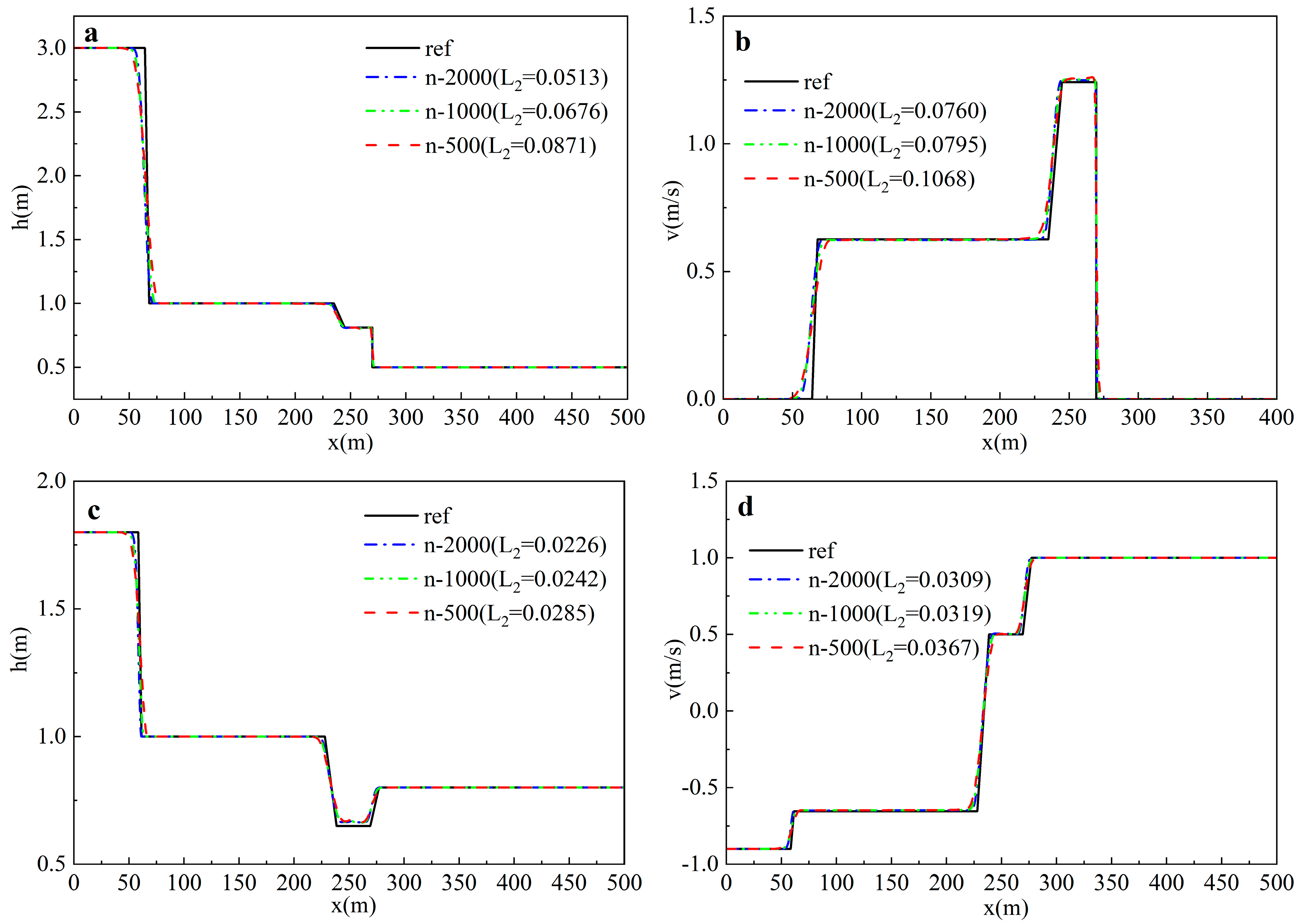
(1)

The initial particle number

The initial particle number is a key parameter in the SPH-PSM model, and its selection significantly impacts the simulation results. As shown in Figure 3, it is evident that increasing the initial particle numbers aligns the transition at the discontinuity ($x=50~60\mathrm{m}$) with the numerical solution, thereby improving the accuracy of the simulation results. When the number of particles is set to 2000, the model achieves the highest accuracy. However, it is important to note that as the initial particle number increases, the computational time required increases exponentially. Therefore, to achieve the desired accuracy, it is advisable to select a proper number of initial particles based on practical applications.

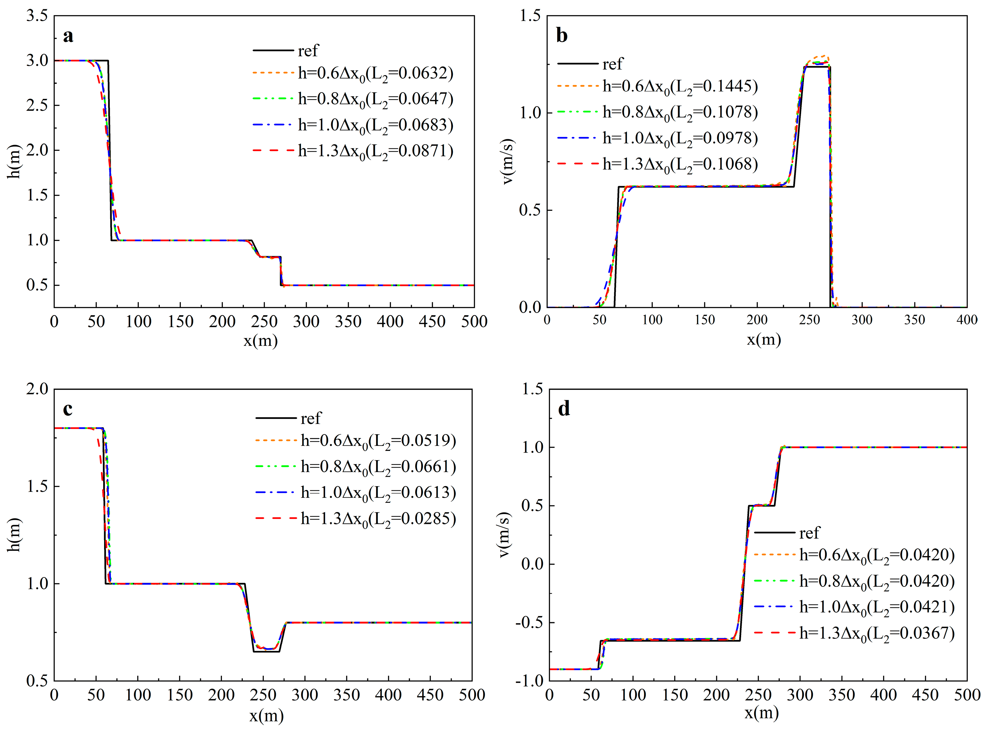
(2)

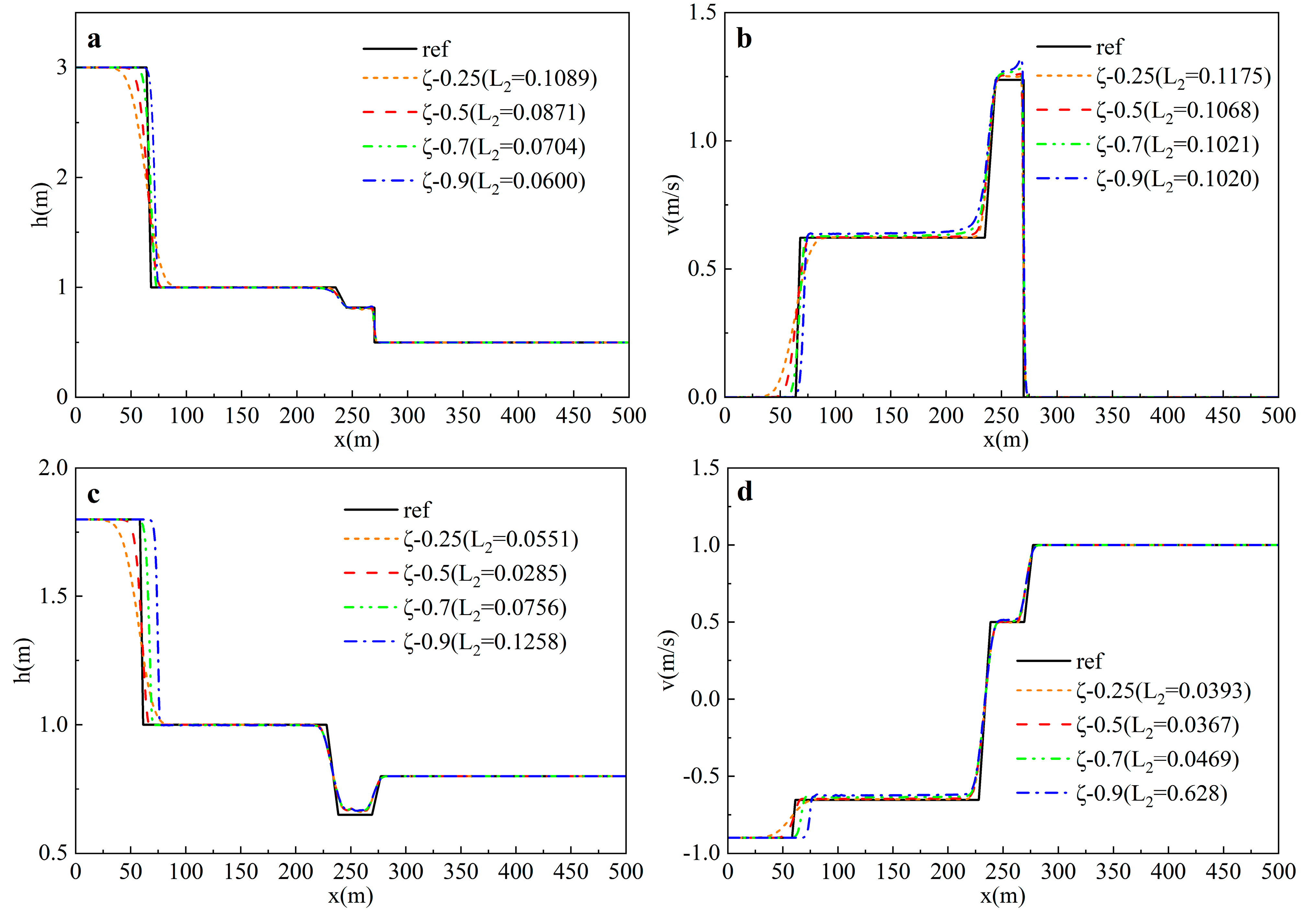
Smoothing Length

In the SPH method, particle properties are obtained by taking a weighted average with neighboring particles. The smoothing length determines the number of neighboring particles within the support domain of each particle. According to Liu and Moubin [31], this section only compared cases where the smoothing length is greater than 0.5$∆x_0$.

Figure 4 shows that using a smoothing length between 0.5$∆x_0$ and 1.0$∆x_0$ results in higher numerical accuracy, as seen in the pressure simulation results of T1. However, in practical pipelines with pipe slope friction and continuous particle movement, using a small smoothing length can lead to a lack of particles within the support domain, which can impact the computational stability of the program. In the more extreme flow condition T2, the simulation accuracy is lower when the smoothing length is less than 1.

When the smoothing length is greater than 1.0$∆x_0$, the support domain includes more particles, resulting in smoother results in abrupt transition conditions (e.g., T2). Likewise, in T1, the simulation accuracy decreases at positions where the smoothing length is greater than 1. Therefore, to balance the stability and the accuracy, the smoothing length around (1.1–1.5)$∆x_0$ is recommended.

(3)

Smoothing Kernel Function

In the SPH-PSM model, the smoothing kernel function determines the weight of the neighboring particles. This study compared the effects of three commonly used smoothing kernel functions–Gaussian, B-spline, and quintic-spline. The accuracy of the B-spline and quintic-spline kernel functions is higher compared to the Gaussian kernel function in the simulation results, as shown in Figure 5. Comparatively, B-spline is widely used in SPH methods due to its high accuracy and concise formula; this study uses B-spline kernel functions for various research cases.

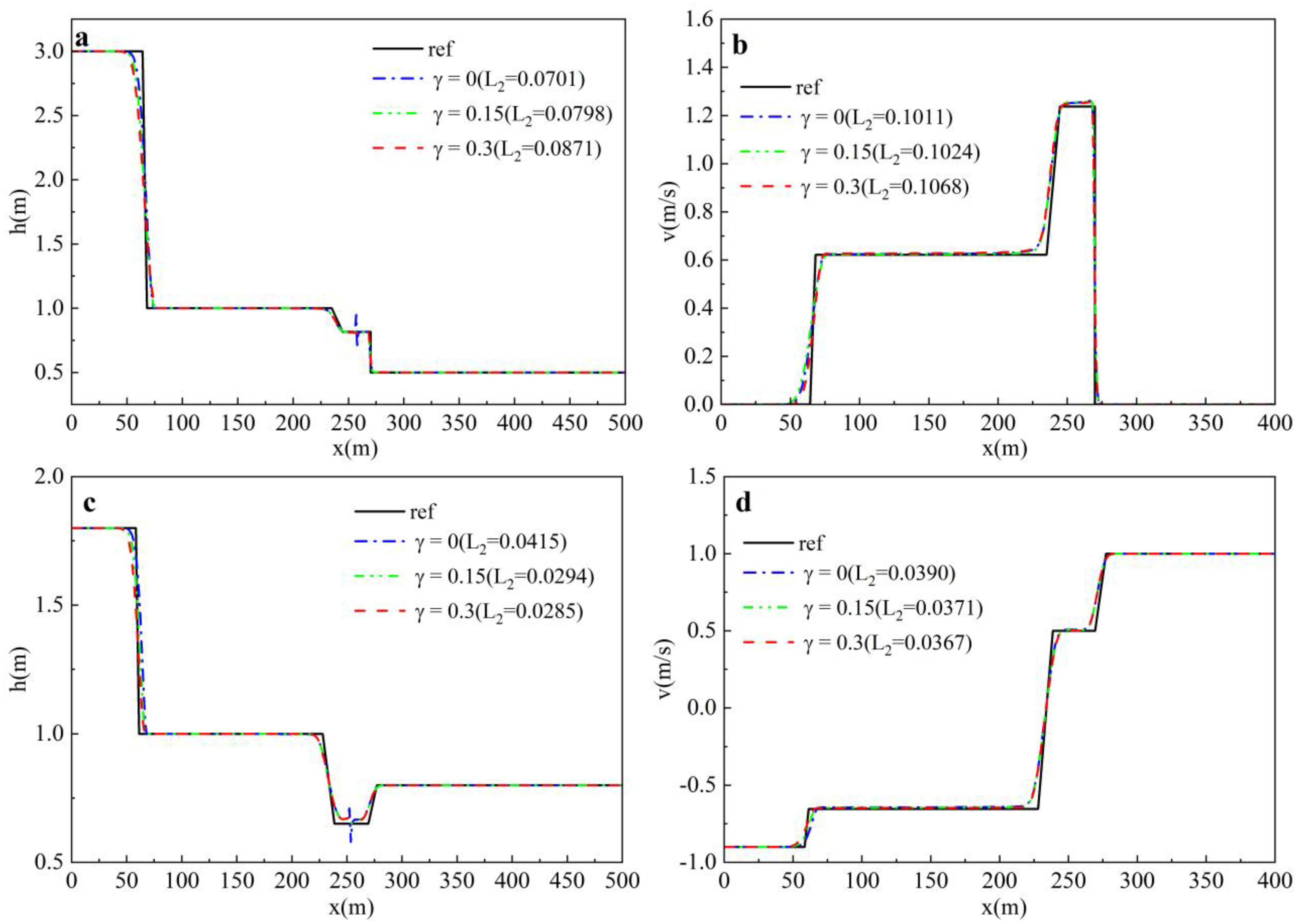
(4)

Density Diffusion Coefficient

The density diffusion coefficient $\gamma$ is used to improve the particle pressure distribution in the SPH method. Therefore, it is necessary to choose a reasonable $\gamma$ during the simulation process. From Figure 6, the influence of the density diffusion coefficient on flow velocity is minor.

In Case T1, as the density diffusion coefficient is increased from 0 to 0.3, the pressure numerical oscillations at the initial discontinuity interface (x = 250 m) decrease due to the suppression effect of $\gamma$ on numerical oscillations from Figure 6. However, this also leads to smoother simulation values in the transition section around 60–70 m, resulting in an overall increase in errors (T1). On the other hand, in Case T2, as the density diffusion coefficient increases, the errors in pressure and velocity gradually decrease. Additionally, the pressure simulation results at the initial discontinuity interface (x = 250 m) also show improvement.

Therefore, the recommended value for the density diffusion coefficient ranges from 0.1 to 0.3 in the SPH-PSM model, while a larger value can be considered in abrupt transition conditions. To ensure stable solving, $\gamma$ was selected as 0.3 for subsequent research, as it effectively suppresses spurious numerical oscillations at the discontinuity interface while maintaining balance and accuracy.

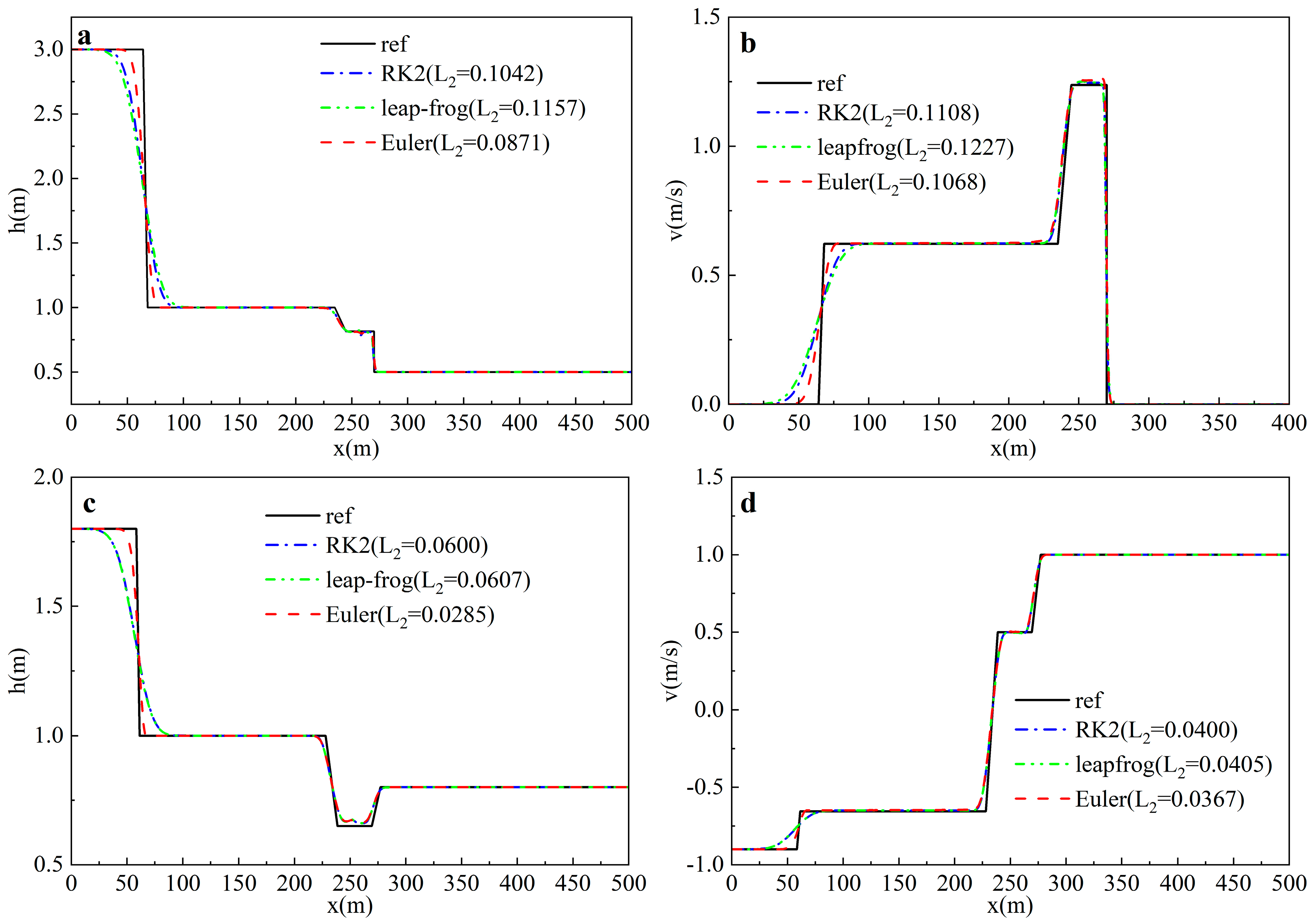
(5)

Time integration scheme

This study discussed the impact of commonly used time integration schemes on the SPH-PSM model, including the Euler method, the leapfrog method, and the second order Runge–Kutta method (RK2).

Based on the findings in Figure 7, it can be observed that the results obtained from the leapfrog method and the RK2 method are quite similar in both cases. However, when it comes to simulating velocity and pressure, the Euler method demonstrates higher accuracy compared to both the leapfrog method and the RK2 method. Furthermore, the Euler method requires less data storage, making it a more efficient choice. Therefore, for the subsequent research in this study, the Euler method was selected as the preferred time integration format.

(6)

Courant number

The Courant number ($\zeta$) determines the time step in numerical simulations. For explicit numerical methods, the value of $\zeta$ is generally not greater than 1; therefore, this study selected 0.25, 0.5, 0.7, and 0.9 for testing.

From Figure 8, it can be observed that the Courant number has a minor impact on the relatively stable T1 case. As the Courant number increases, the error in piezometric head and velocity even decreases. On the contrary, for the T2 case, when the Courant numbers are greater than 0.5, the simulation result completely deviates from the reference solution of the regime transition interface ($x=50~60\mathrm{m}$). This deviation results in gradual increases in errors in pressure and velocity, as shown. The complex hydrodynamic conditions, including opposite flow in T2, require a low Courant number for numerical accuracy and stability. As shown in

Table 2. The CPU time for different Courant numbers in various cases.

$\mathit{\zeta }$	0.25	0.5	0.7	0.9
CPU time(s) of T1	4.8606	1.3216	1.0365	0.9318
CPU time(s) of T2	2.9158	0.9700	0.6997	0.6245

, a smaller Courant number leads to longer computational time and higher computational cost. Therefore, to strike a balance between stability, accuracy, and computational cost, it is recommended to use a Courant number ($\zeta$) less than 0.5 for the SPH-PSM model.

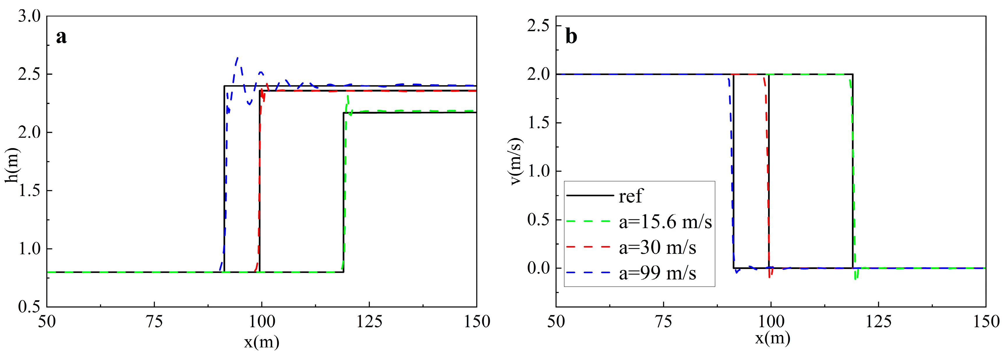
3.1.2. PSM-Related Parameters

The parameters related to PSM are the slot width and the pressure wave celerity. However, when the cross-sectional area of the pipeline is determined, $T_S$ and $a$ can be simplified to a single variable parameter according to Equation (2). Generally, to avoid spurious numerical oscillations caused by flow regime transitions, the slot width is usually set to 1–2% of the pipe diameter [2]. Since the slot width is affected by various factors such as the shape of the cross-section, this paper focuses on discussing the pressure wave celerity as an intrinsic influence to ensure the generalizability of the results.

T3 is selected as the benchmark case for the study of PSM-related parameters. In this study, the pressure wave celerity discussed were 99 m/s, 31 m/s, and 15.6 m/s, corresponding to the slot widths of 0.001 m, 0.01 m, and 0.04 m, respectively.

The initial condition of T3 involves two free-surface flows with equal piezometric heads and opposite velocities. When these flows collide, shock waves are generated, resulting in pressurized flows. As the pressure wave celerity increases to 99 m/s, the numerical oscillation becomes apparent and the pressure after collision increases, as shown in Figure 9. Meanwhile, the flow regime transition position moves closer to the upstream and downstream boundaries. Comparing the simulation results in Figure 9, it is clear that as the pressure wave celerity increases, the magnitude of the pressure increases and the advance in the shock position gradually decreases.

When selecting pressure wave celerity, it is necessary to consider the numerical oscillation caused by the narrow slot and the distortion of the simulation results due to the wide slot. The pressure wave celerity of around 30 m/s was found to produce satisfactory simulation results according to Figure 9.

3.2. Numerical Case Validation

In this section, the proposed SPH-PSM model is validated in different flow regimes. The recommended model parameters were used based on the parameter discussion above with a smoothing length of 1.3$∆x_0$, B-spline as the kernel function, the density diffusion coefficient of 0.3, Euler integration with a Courant number of 0.5, and the pressure wave celerity is 30 m/s. The particle number is determined by the specific case.

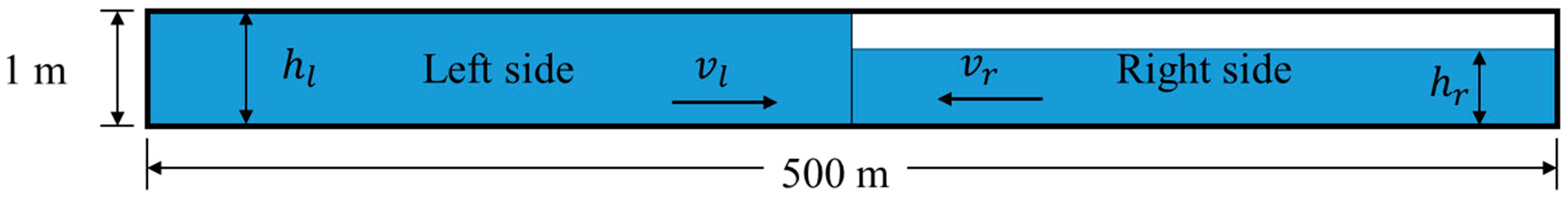
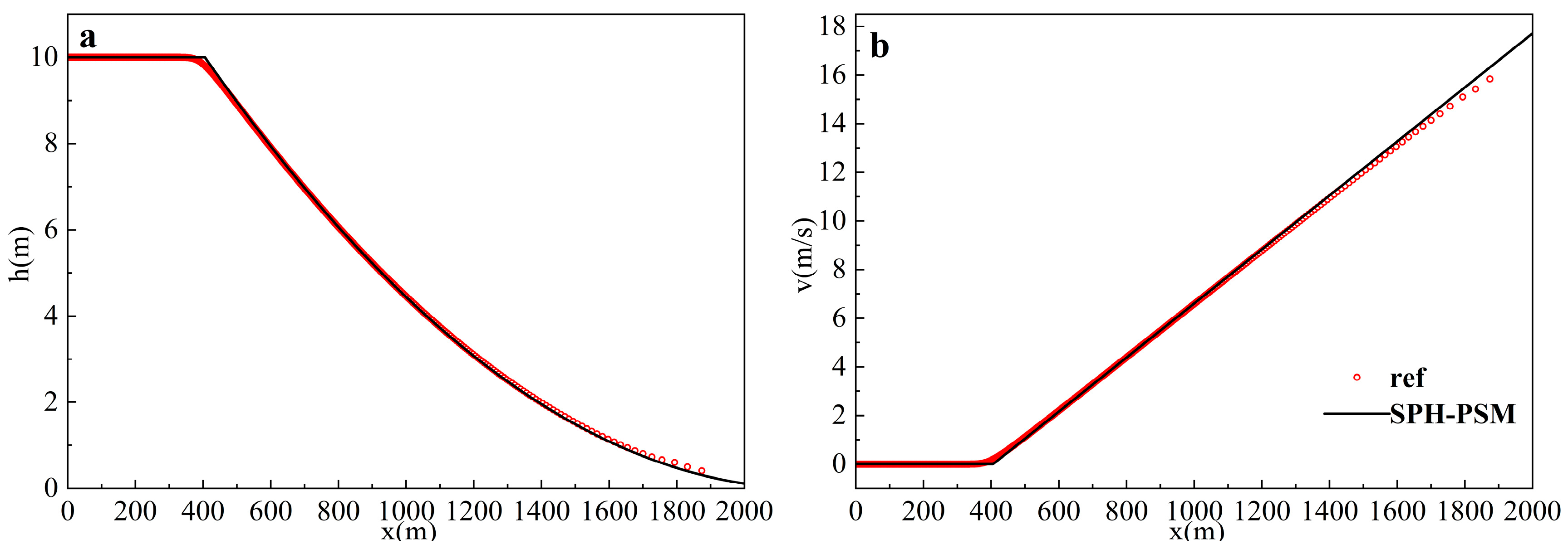
3.2.1. Case 1: Dam-Break Case

Dam-break flow cases can be used to test the capability of the SPH-PSM model to simulate single open-channel flow and handle wet–dry interface discontinuities. In this hypothetical example, a horizontal, frictionless fluid with a length of 2000 m is considered. The dam is located at 1000 m, with an initial upstream water depth of 10 m and downstream water depth of 0 m. At $t$ = 0, the dam collapses.

For this specific case, initial particle number $N$ was set as 500 (initial spacing ${∆x}_0$ is 4 m), while the simulation duration is 60 s. To validate the accuracy of the model, the theoretical solution from Issakhov et al. [44] was utilized as a reference for the dam-break case.

$$\begin{array}{c}\left\{\begin{array}{c}h\left(x,t\right)=\frac{1}{9g}{\left[2\sqrt{g{h}_0}-\frac{x}{t}\right]}^2\\ v\left(x,t\right)=\frac{2}{3}\left[\sqrt{g{h}_0}+\frac{x}{t}\right]\end{array}\right.\end{array}$$

(13)

where $h$ is the water depth; $h_0$ is the upstream water depth; $t$ is time; $x$ is the coordinate, with positive direction pointing downstream from the dam; $v$ is the average flow velocity at the cross-section of the river; and $g$ is the gravitational acceleration.

Figure 10 illustrates a comparison of the simulation results of water depth and flow velocity in the channel with the analytical solution. As seen in Figure 10, the numerical solution closely aligns with the theoretical solution, indicating the effectiveness of the established dam-break numerical model. These results demonstrate that the SPH-PSM model accurately reproduces the hydraulic conditions of one-dimensional open channels and effectively handles wet–dry interfaces. Overall, this confirms the model’s capability for simulating open-channel flow and its potential for widespread use in related applications.

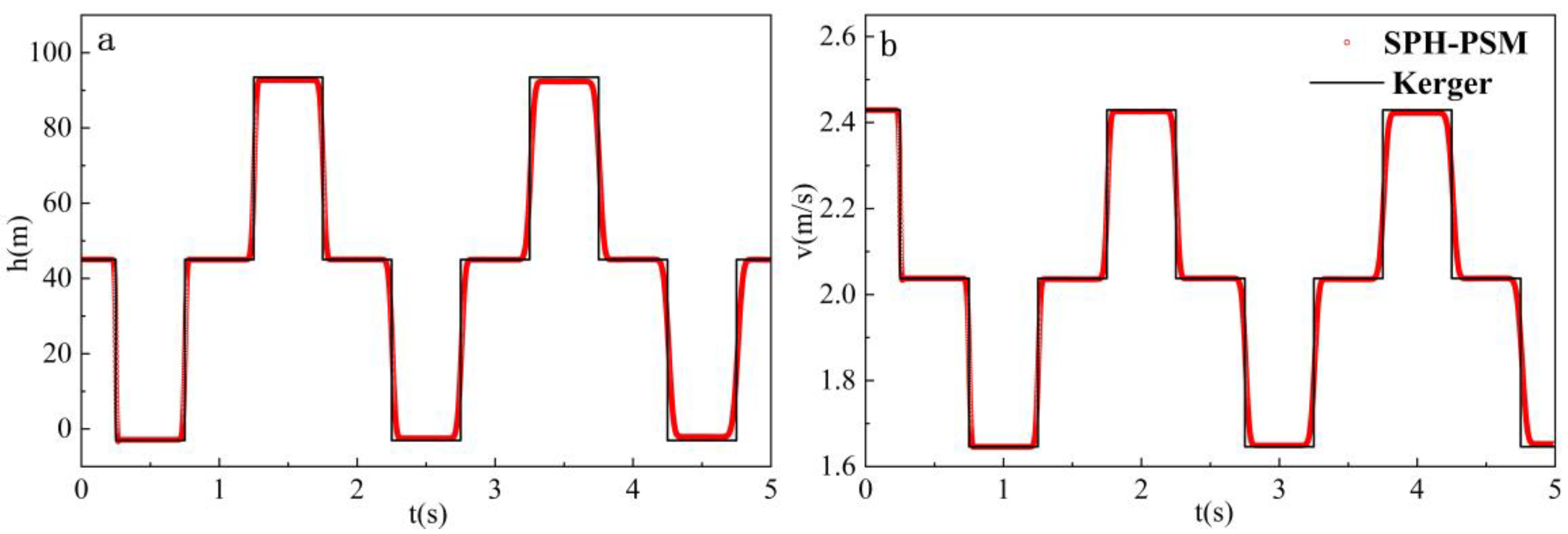
3.2.2. Case 2: Water Hammer Cases

Water hammer cases are conducted to evaluate the SPH-PSM model’s ability to simulate pressurized flow and accurately capture negative pressure occurrences in pipelines. In this scenario, a circular pipe with a length of 600 m and a diameter of 0.5 m is considered. Friction in the pipeline is neglected, and the pipe is horizontal. The transient event is triggered by an instantaneous change in the upstream flow rate from 0.477 m³/s to 0.4 m³/s, while a downstream water tank maintains a constant water pressure of 45 m.

The initial number of particles was 600 (the initial spacing is 1 m). No regime transition is involved in the water hammer case, so a physically meaningful pressure wave celerity of 1200 m/s was used to improve accuracy, corresponding to a slot width of 1.334 × 10⁻⁶ m and the simulation duration was 5 s.

The analytical solution for the water hammer case, as referenced by Kerger et al. [17], predicts a pressure oscillation of approximately 48.05 m following the mentioned change in flow rate. As shown in Figure 11, the simulation results of the SPH-PSM model show good agreement with the analytical solution. The model accurately simulates negative pressure situations and reproduces the propagation process of pressure and flow rate oscillations, including their amplitude, period, and phase.

3.2.3. Mixed Flow Cases

(1)

Case 3: Pipeline Valve Rapid Closure Case

The idealistic test proposed by Dazzi et al. [43] allows for a comparative analysis between SPH-PSM and mesh-based methods. The reference solution of text is based on a fine grid numerical (2000 grids, $∆x_0$ = 0.05 m).

The case involves a circular pipe with a length of 100 m, a diameter of 1 m, a slope of 0.4%, and a Manning coefficient of 0.015. The initial flow in the pipe is 0.7 m³/s, with an initial water level of 0.52 m. The pipe pressurization occurs due to the sudden closure of a downstream valve (at t = 0 s).

The particle numbers were as follows: (a) 100 particles ($∆x_0$ = 1 m); (b) 2000 particles ($∆x_0$ = 0.05 m), and simulation duration is 60 s. The upstream flow rate is 0.7 m³/s, and the downstream is a solid wall boundary.

Figure 12 presents the simulation results of the piezometric head at different time steps. Regarding the motion of the free surface and pressurized interface, it can be observed from the figure that, as the downstream valve is closed at t = 0 while normal inflow continues from the upstream, the downstream water level gradually rises to a full pipe flow state. This results in the appearance of a interface between the free surface and the pressurized interface, and with the passage of time, this interface gradually moves upstream. It is evident that the SPH-PSM model successfully simulates the continuous free surface/pressurized interface, accurately describing the movement of the interface and the corresponding pressure.

When simulating with 100 particles, the pressure at the flow regime transition interface appears to be relatively smooth. The simulation results with 100 particles can also accurately reflect the motion of free surfaces, pressurized interface, and the water level after pressurization in the model. Increasing the number of particles to 2000 leads to a more accurate simulation that better captures the abrupt change in pressure at the flow regime transition interface. From the results, it is evident that a finer particle subdivision yields more accurate simulation results. This finding is consistent with the analysis presented in Section 3.1.1.

(2)

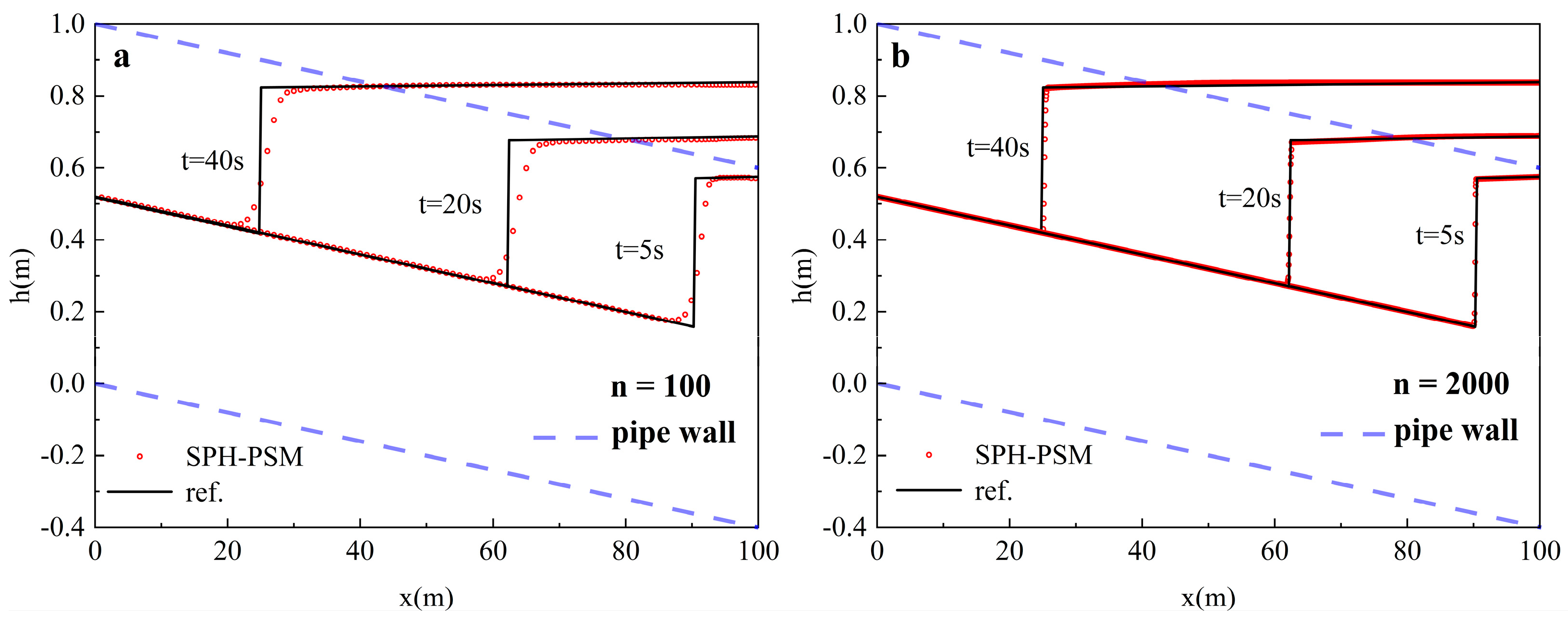
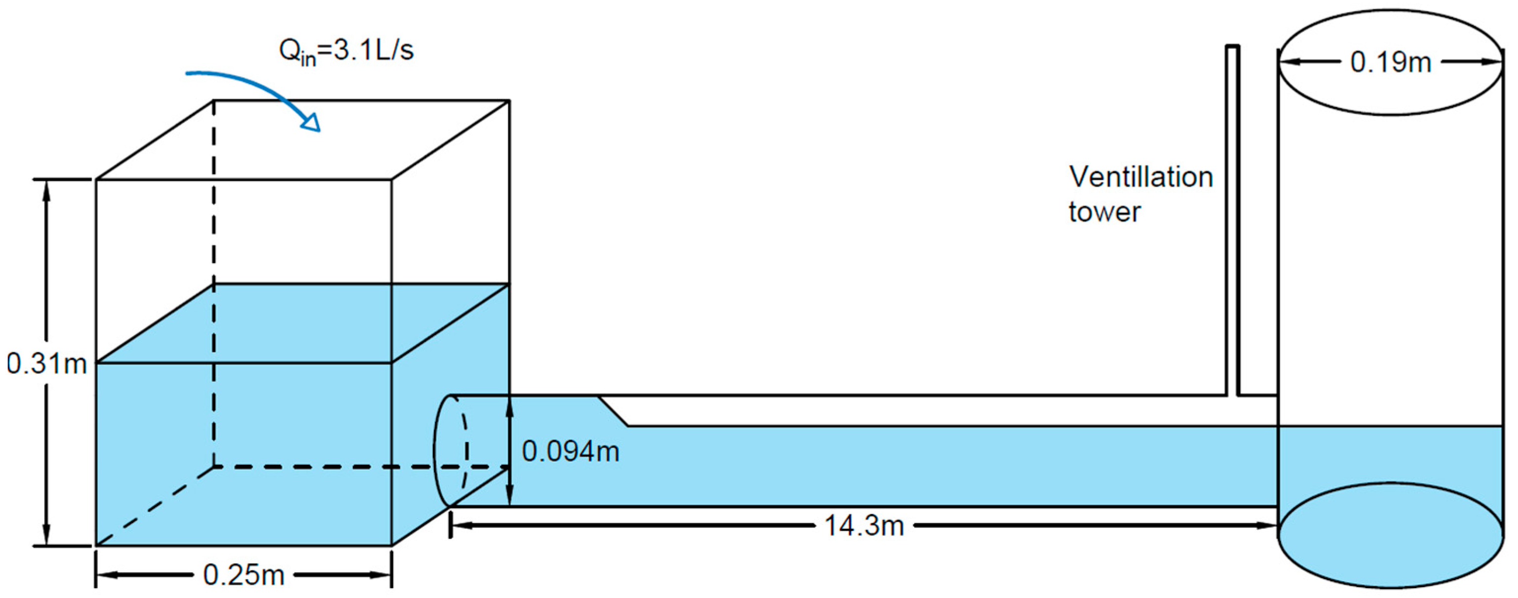
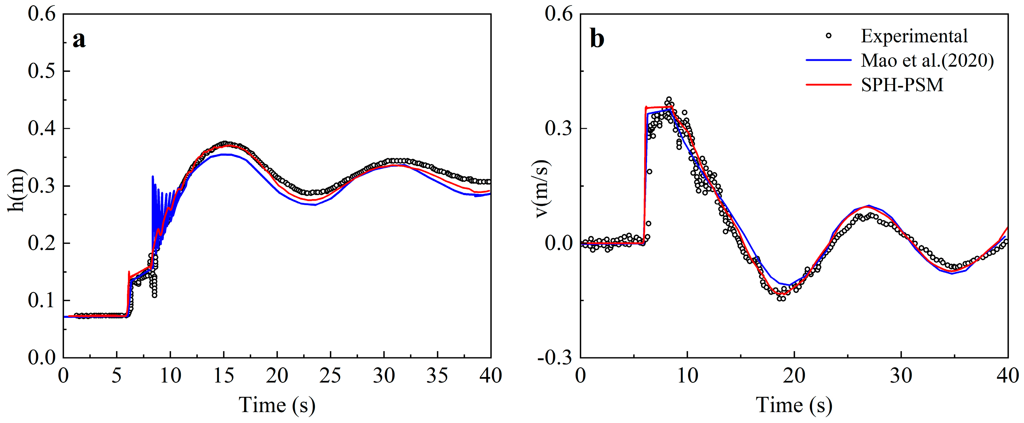
Case 4: Single Drainage Pipe Case

The experimental setup designed by Vasconcelos et al. [3] simulates a simplified “stormwater well-pipe-stormwater well” system. In this case, water continuously flows into the upstream, and both upstream and downstream are open boundaries. The method of characteristics is employed to solve boundary conditions.

As shown in Figure 13, the experimental setup consists of an upper and lower stormwater well connected by a pipe. The horizontal pipe is 14.33 m long with a diameter of 0.094 m. The upstream stormwater well measures 0.31 m in height and has a square bottom with dimensions of 0.25 m by 0.25 m. The down stormwater well is designed with a circular bottom, with a height sufficient to prevent water overflow and a bottom diameter of 0.19 m. The Manning coefficient is 0.012. A gate located downstream of the pipe is installed. To eliminate the impact of trapped air within the system on the experiment, a ventilation pipe is arranged near the gate.

The initial water depth in the experiment is 0.073 m and a constant inflow of 3.1 L/s is set at the upstream rainwater well. Water exceeding the height of the upstream rainwater well will overflow from the top of the pipe. Pressure and velocity data were measured 9.9 m away from the upstream boundary. The initial spacing of particles is 0.1 m. The simulation duration is 40 s.

It is worth noting that the experiment described a partially closed gate at the downstream end of the pipeline. This partial closure may restrict water flow, thereby reducing the observed oscillations in the experiment and slowing down the propagation speed of pressure waves upstream. Therefore, we modified the model by adding a local head loss term $h_f$to roughly account for the gate’s influence, as follows:

$$\begin{array}{c}{h}_f={\left(\xi \right)}^2\frac{v^2}{2g}\end{array}$$

(14)

As per the reference literature [45], when the local head loss coefficient $\xi$ = 25, the modified simulation results achieved better consistency.

As shown in Figure 14, the phases of the oscillations are essentially the same, but the model underpredicts the damping of the subsequent oscillations. These discrepancies may be attributed to an underestimation of energy losses [3] during the simulation process or constant pressure wave celerity [15]. Although there are differences in pressure simulation, considering that existing models also exhibit such differences, we deem this difference acceptable [3,38,46].

Overall, the SPH-PSM model can effectively reproduce satisfying results of the classical numerical and experimental cases when compared to the reference data from the literature. The recommended optimal parameters of the proposed model prove to be effective in addressing different flow conditions.

4. Conclusions

In this study, a one-dimensional pipeline transient mixed-flow model called the SPH-PSM model is established by combining smoothed particle hydrodynamic methods and the Preissmann slot method. Subsequently, the empirical parameters within the SPH-PSM model are systematically tested and discussed. Finally, the proposed model with optimal parameters is validated with classic numerical and experimental cases from the literature. The key findings are summarized as follows:

(1)

The newly proposed SPH-PSM model demonstrates its effectiveness in accurately simulating complex transient flow regimes.

(2)

The recommended model parameters for SPH-PSM are specified as follows: (a) the B-spline kernel function is more appropriate in the SPH-PSM model; (b) the recommended smoothing length is (1.1–1.5)$∆x_0$ to balance stability and accuracy; (c) the density diffusion coefficient $\gamma$ can suppress the numerical oscillations while potentially compromising mass conservation, which is recommended as 0.1–0.3, while a larger $\gamma$ is recommended for intense mixed flows; (d) among different numerical integration methods, the Euler method proves to be superior in terms of computation time and accuracy; (e) to maintain a balance between stability, accuracy, and efficiency, a Courant number less than 0.5 is recommended; (f) the choice of pressure wave celerity affects not only the numerical oscillation but also the position of the shock and the piezometric head, which is recommended as 30 m/s; meanwhile, in the pure pressurized flow, the true acoustic velocity should be chosen to ensure accuracy.

In conclusion, the proposed SPH-PSM model exhibits its versatility in simulating transient mixed flows within pipelines. It provides an alternative approach to modeling pipe fluid dynamics. Attributable to the mesh-free nature of SPH, the SPH-PSM model can be further extended to solve multiphase flow issues like entrapped air pockets and sediment transport in future research.

References

- Aureli, F.; Dazzi, S.; Maranzoni, A.; Mignosa, P. Validation of single- and two-equation models for transient mixed flows: A laboratory test case. J. Hydraul. Res. 2015, 53, 440–451. [Google Scholar] [CrossRef]
- Trajkovic, B.; Ivetic, M.; Calomino, F.; D’Ippolito, A. Investigation of transition from free surface to pressurized flow in a circular pipe. Water Sci. Technol. 1999, 39, 105–112. [Google Scholar] [CrossRef]
- Vasconcelos, J.G.; Wright, S.J.; Roe, P.L. Improved simulation of flow regime transition in sewers: Two-component pressure approach. J. Hydraul. Eng. 2006, 132, 553–562. [Google Scholar] [CrossRef]
- Chitwatkulsiri, D.; Miyamoto, H. Real-Time Urban Flood Forecasting Systems for Southeast Asia—A Review of Present Modelling and Its Future Prospects. Water 2023, 15, 178. [Google Scholar] [CrossRef]
- Elliott, A.H.; Trowsdale, S.A. A review of models for low impact urban stormwater drainage. Environ. Modell. Softw. 2007, 22, 394–405. [Google Scholar] [CrossRef]
- Farina, A.; Di Nardo, A.; Gargano, R.; van der Werf, J.A.; Greco, R. A simplified approach for the hydrological simulation of urban drainage systems with SWMM. J. Hydrol. 2023, 623, 129757. [Google Scholar] [CrossRef]
- Bousso, S.; Daynou, M.; Fuamba, M. Numerical Modeling of Mixed Flows in Storm Water Systems: Critical Review of Literature. J. Hydraul. Eng. 2013, 139, 385–396. [Google Scholar] [CrossRef]
- Li, F.; Yan, J.; Yan, H.; Tao, T.; Duan, H.-F. 2D Modelling and energy analysis of entrapped air-pocket propagation and spring-like geysering in the drainage pipeline system. Eng. Appl. Comput. Fluid Mech. 2023, 17, 2227662. [Google Scholar] [CrossRef]
- Cunge, J.A.; Wegner, M. Numerical integration of Barré de Saint-Venant’s flow equations by means of an implicite scheme of finite differences. La Houille Blanche 1964, 50, 33–39. [Google Scholar] [CrossRef]
- Kerger, F.; Archambeau, P.; Erpicum, S.; Dewals, B.J.; Pirotton, M. A fast universal solver for 1D continuous and discotinuous steady flows in rivers and pipes. Int. J. Numer. Methods Fluids 2011, 66, 38–48. [Google Scholar] [CrossRef]
- Li, J.; McCorquodale, A. Modeling mixed flow in storm sewers. J. Hydraul. Eng. 1999, 125, 1170–1180. [Google Scholar] [CrossRef]
- Huang, B.; Zhu, D.Z. Rigid-column model for rapid filling in a partially filled horizontal pipe. J. Hydraul. Eng. 2021, 147, 06020018. [Google Scholar] [CrossRef]
- An, H.; Lee, S.; Noh, S.J.; Kim, Y.; Noh, J. Hybrid Numerical Scheme of Preissmann Slot Model for Transient Mixed Flows. Water 2018, 10, 899. [Google Scholar] [CrossRef]
- Henau, V.D.; Raithby, G. A transient two-fluid model for the simulation of slug flow in pipelines—II. Validation. Int. J. Multiph. Flow 1995, 21, 351–364. [Google Scholar] [CrossRef]
- Sharior, S.; Hodges, B.; Vasconcelos, J.G. Generalized, Dynamic, and Transient-Storage Form of the Preissmann Slot. J. Hydraul. Eng. 2023, 149, 04023046. [Google Scholar] [CrossRef]
- León, A.S.; Ghidaoui, M.S.; Schmidt, A.R.; García, M.H. Godunov-type solutions for transient flows in sewers. J. Hydraul. Eng. 2006, 132, 800–813. [Google Scholar] [CrossRef]
- Kerger, F.; Archambeau, P.; Erpicum, S.; Dewals, B.J.; Pirotton, M. An exact Riemann solver and a Godunov scheme for simulating highly transient mixed flows. J. Comput. Appl. Math. 2011, 235, 2030–2040. [Google Scholar] [CrossRef]
- Chaudhry, M.H. Open-Channel Flow; Springer: Berlin/Heidelberg, Germany, 2008; Volume 523. [Google Scholar]
- Ye, T.; Pan, D.; Huang, C.; Liu, M. Smoothed particle hydrodynamics (SPH) for complex fluid flows: Recent developments in methodology and applications. Phys. Fluids 2019, 31, 011301. [Google Scholar] [CrossRef]
- Monaghan, J.J. Simulating free surface flows with SPH. J. Comput. Phys. 1994, 110, 399–406. [Google Scholar] [CrossRef]
- Swegle, J.; Attaway, S. On the feasibility of using smoothed particle hydrodynamics for underwater explosion calculations. Comput. Mech. 1995, 17, 151–168. [Google Scholar] [CrossRef]
- Salis, N.; Luo, M.; Reali, A.; Manenti, S. Wave generation and wave-structure impact modelling with WCSPH. Ocean Eng. 2022, 266, 113228. [Google Scholar] [CrossRef]
- Chang, T.J.; Chang, K.H. SPH Modeling of One-Dimensional Nonrectangular and Nonprismatic Channel Flows with Open Boundaries. J. Hydraul. Eng. 2013, 139, 1142–1149. [Google Scholar] [CrossRef]
- Chang, K.H.; Chang, T.J. A well-balanced and positivity-preserving SPH method for shallow water flows in open channels. J. Hydraul. Res. 2021, 59, 903–916. [Google Scholar] [CrossRef]
- Pan, T.W.; Zhou, L.; Ou, C.Q.; Wang, P.; Liu, D.Y. Smoothed Particle Hydrodynamics with Unsteady Friction Model for Water Hammer Pipe Flow. J. Hydraul. Eng. 2022, 148, 04021057. [Google Scholar] [CrossRef]
- Wieth, L.; Kelemen, K.; Braun, S.; Koch, R.; Bauer, H.J.; Schuchmann, H.P. Smoothed Particle Hydrodynamics (SPH) simulation of a high-pressure homogenization process. Microfluid. Nanofluid 2016, 20, 42. [Google Scholar] [CrossRef]
- Zhou, M.J.; Shi, Z.M.; Peng, C.; Peng, M.; Cui, K.F.E.; Li, B.; Zhang, L.M.; Zhou, G.G.D. Two-phase modelling of erosion and deposition process during overtopping failure of landslide dams using GPU-accelerated ED-SPH. Comput. Geotech. 2024, 166, 105944. [Google Scholar] [CrossRef]
- Nomeritae, N.; Bui, H.H.; Daly, E. Modeling Transitions between Free Surface and Pressurized Flow with Smoothed Particle Hydrodynamics. J. Hydraul. Eng. 2018, 144, 04018012. [Google Scholar] [CrossRef]
- Song, W.K.; Yan, H.X.; Tao, T.; Guan, M.F.; Li, F.; Xin, K.L. Modeling Transient Mixed Flows in Drainage Networks With Smoothed Particle Hydrodynamics. Water Resour. Manag. 2024, 38, 861–879. [Google Scholar] [CrossRef]
- Preissmann, A. Propagation des Intumescences Dans Lescanaux et Rivieres; 1st Cong. French Assoc. for Computation: Grenoble, France, 1961. [Google Scholar]
- Liu, G.-R.; Liu, M.B. Smoothed Particle Hydrodynamics: A Meshfree Particle Method; World Scientific: Singapore, 2003. [Google Scholar]
- Bonet, J.; Lok, T.S.L. Variational and momentum preservation aspects of Smooth Particle Hydrodynamic formulations. Comput. Methods Appl. Mech. Eng. 1999, 180, 97–115. [Google Scholar] [CrossRef]
- Chen, J.K.; Beraun, J.E.; Carney, T.C. A corrective smoothed particle method for boundary value problems in heat conduction. Int. J. Numer. Methods Eng. 1999, 46, 231–252. [Google Scholar] [CrossRef]
- Monaghan, J.J.; Gingold, R.A. Shock Simulation by the Particle Method Sph. J. Comput. Phys. 1983, 52, 374–389. [Google Scholar] [CrossRef]
- Lahiri, S.K.; Bhattacharya, K.; Shaw, A.; Ramachandra, L.S. A stable SPH with adaptive B-spline kernel. J. Comput. Phys. 2020, 422, 109761. [Google Scholar] [CrossRef]
- Yang, X.F.; Peng, S.L.; Liu, M.S. A new kernel function for SPH with applications to free surface flows. Appl. Math. Model. 2014, 38, 3822–3833. [Google Scholar] [CrossRef]
- Ata, R.; Soulaïmani, A. A stabilized SPH method for inviscid shallow water flows. Int. J. Numer. Methods Fluids 2005, 47, 139–159. [Google Scholar] [CrossRef]
- Chang, K.H.; Sheu, T.W.H.; Chang, T.J. A 1D-2D coupled SPH-SWE model applied to open channel flow simulations in complicated geometries. Adv. Water Resour. 2018, 115, 185–197. [Google Scholar] [CrossRef]
- Vacondio, R.; Rogers, B.; Stansby, P. Smoothed Particle Hydrodynamics: Approximate zero-consistent 2-D boundary conditions and still shallow-water tests. Int. J. Numer. Methods Fluids 2012, 69, 226–253. [Google Scholar] [CrossRef]
- Mabssout, M.; Herreros, M.I. Runge-Kutta vs Taylor-SPH: Two time integration schemes for SPH with application to Soil Dynamics. Appl. Math. Model. 2013, 37, 3541–3563. [Google Scholar] [CrossRef]
- Federico, I.; Marrone, S.; Colagrossi, A.; Aristodemo, F.; Antuono, M. Simulating 2D open-channel flows through an SPH model. Eur. J. Mech.-B/Fluids 2012, 34, 35–46. [Google Scholar] [CrossRef]
- Song, W.K.; Yan, H.X.; Li, F.; Tao, T.; Duan, H.F.; Xin, K.L.; Li, S.P. Development of Smoothed Particle Hydrodynamics based water hammer model for water distribution systems. Eng. Appl. Comput. Fluid Mech. 2023, 17, 2171139. [Google Scholar] [CrossRef]
- Dazzi, S.; Maranzoni, A.; Mignosa, P. Local time stepping applied to mixed flow modelling. J. Hydraul. Res. 2016, 54, 145–157. [Google Scholar] [CrossRef]
- Issakhov, A.; Zhandaulet, Y.; Abylkassymova, A. Numerical Study of the Water Surface Movement during a Dam Break on a Slope with Cascade Dike from Sediment. Water Resour. Manag. 2022, 36, 3435–3461. [Google Scholar] [CrossRef]
- Sanders, B.F.; Bradford, S.F. Network implementation of the two-component pressure approach for transient flow in storm sewers. J. Hydraul. Eng. 2011, 137, 158–172. [Google Scholar] [CrossRef]
- Mao, Z.H.; Guan, G.H.; Yang, Z.H. Suppress Numerical Oscillations in Transient Mixed Flow Simulations with a Modified HLL Solver. Water 2020, 12, 1245. [Google Scholar] [CrossRef]