Global Events and Surge in Residential Water Demand: Exploring Possible Hydraulic Scenarios

 ,
,  ,
,  ,
,  and
and 
Abstract
:1. Introduction
2. Methodology
2.1. Description of the Combinations and Scenarios
2.1.1. Peak Water Consumption
2.1.2. Water Consumption Due to Climate Change—Qcc
2.1.3. Water Consumption Due to SarsCoV; Qcov10 and Qcov40 Increase
2.1.4. Water Consumption Due to Population Growth—QPG
2.1.5. Water Consumption Due to Fire—QF
2.2. Case Study
3. Results
3.1. Discussion of Results
3.1.1. Global Influences on Water Consumption Patterns
3.1.2. Water Efficiency Trends: Motivating Sustainable Reduction in Per-Capita Water Use
3.1.3. Implications for Water Distribution Network Design
3.1.4. Water Infrastructure Optimization
3.2. Limitations
4. Conclusions
Author Contributions
Funding
Data Availability Statement
Conflicts of Interest
Appendix A. Mathematical Details of the Water Consumption Projection Model


| Combination | Denominator Factor for T(s) for 2030 (β2030) | ∫ T(y) dy | Factor to the Year | Denominator Factor for T(s) for 2050 (β2050) | ∫ T(y) dy | Factor to the Year |
|---|---|---|---|---|---|---|
| 2030 | 2050 | |||||
| A | 530.7973 | 0.320139 | 1.33000 | 534.09613 | 0.536935 | 1.55000 |
| B | 270.6562 | 0.627841 | 1.64000 | 217.37157 | 1.319285 | 2.33900 |
| C | 233.7081 | 0.727099 | 1.74000 | 202.17607 | 1.418442 | 2.43900 |
| D | 198.1211 | 0.857703 | 1.87158 | 165.61564 | 1.731570 | 2.75479 |
| E | 147.0637 | 1.155479 | 2.17158 | 141.33525 | 2.029041 | 3.05479 |
Appendix B. Modeling Water Demand Growth as a Product of Population and per Capita Consumption Trends
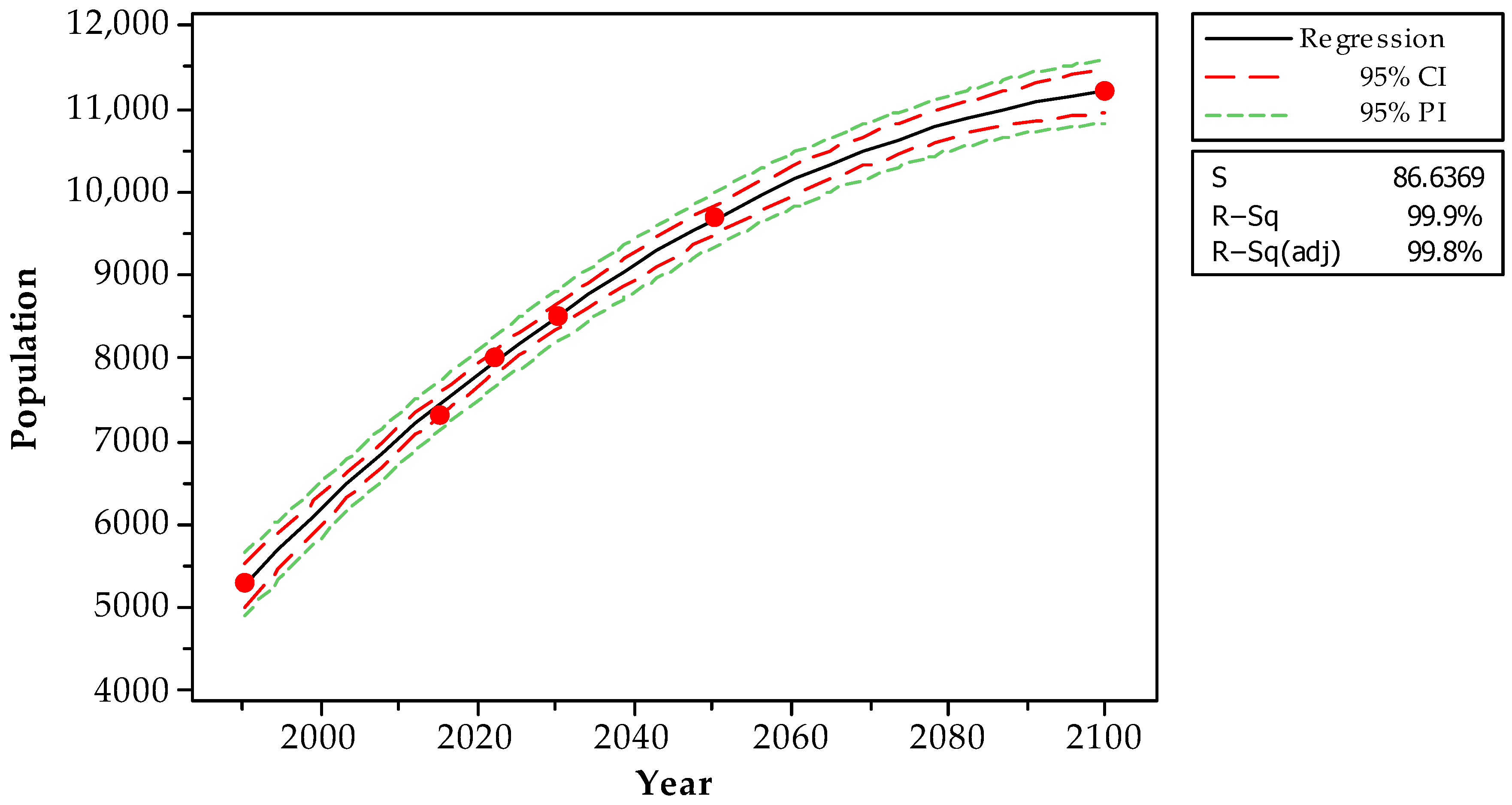
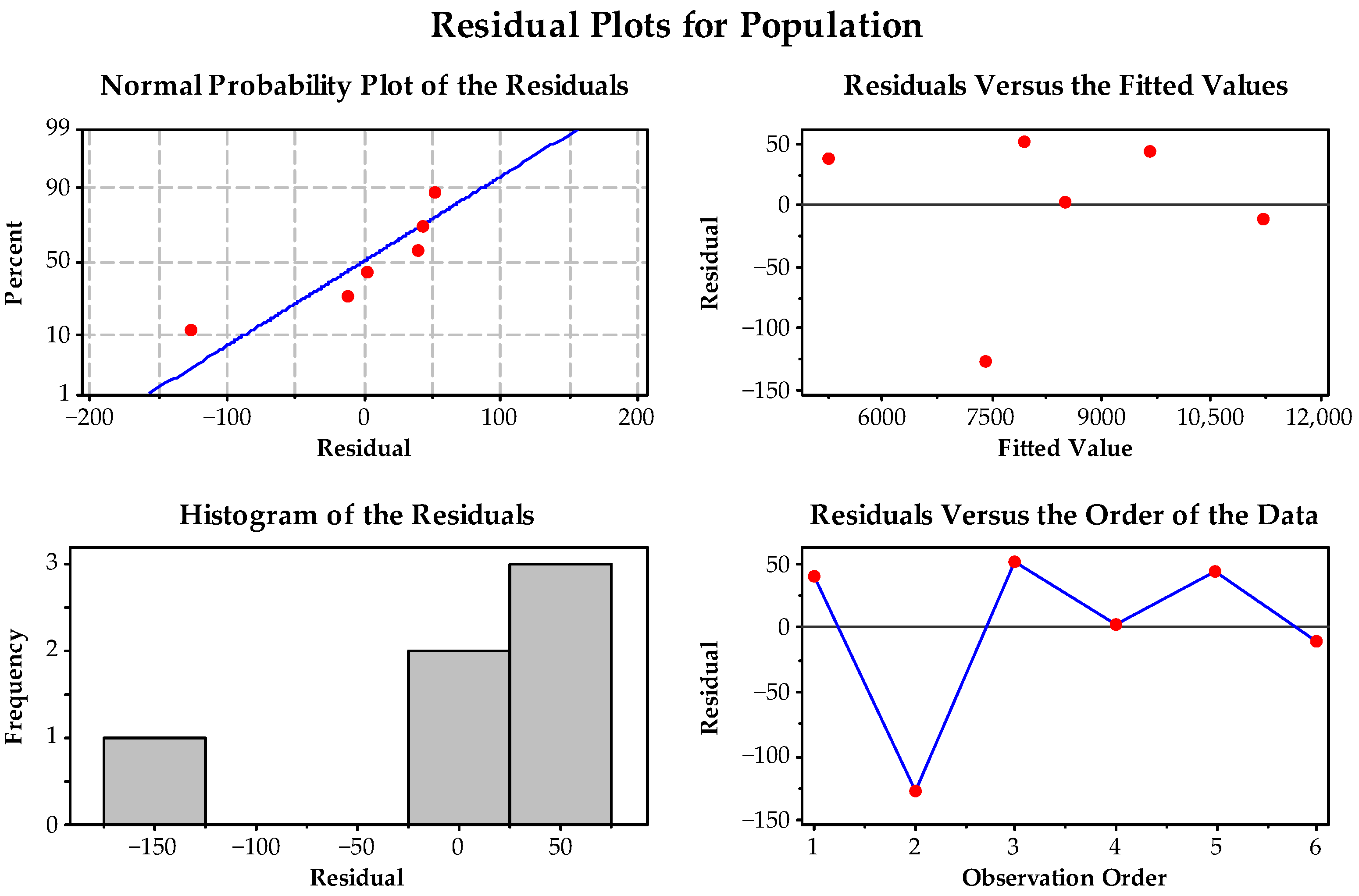
| Year | Population | ∫ P′(y) | ∫ C′(y) | ∫ P′(y) × ∫ C′(y) |
|---|---|---|---|---|
| 1990 | 5300 | 0.0000 | −0.2703 | |
| 2015 | 7300 | 0.1742 | 0.2147 | 0.037 |
| 2022 | 8000 | 0.2161 | 0.3505 | 0.076 |
| 2030 | 8500 | 0.2602 | 0.5056 | 0.132 |
| 2050 | 9700 | 0.3534 | 0.8936 | 0.316 |
| 2100 | 11,200 | 0.4785 | 1.8636 | 0.892 |
References
- Data Commons 2024, Place Explorer. Demographics, Data Commons. Available online: https://datacommons.org/place/Earth?category=Demographics (accessed on 3 March 2024).
- Population Division, Department of Economic and Social Affairs, United Nations. World Population Prospects: The 2012 Revision, Key Findings and Advance Tables; Working Paper No. ESA/P/WP.227; Population Division, Department of Economic and Social Affairs, United Nations: New York, NY, USA, 2013. [Google Scholar]
- UN Water. Water for a Sustainable World. Data and Figures. United Nations Report on World Water Resources. United Nations Educational, Scientific and Cultural Organization. World Water Assessment Programme; UN Water: Geneva, Switzerland, 2015. [Google Scholar]
- UN Water. UN-Water Policy Report on Climate Change and Water. SWEDEN. Swiss Agency for Development and Cooperation SDC. Ministry of Foreign Affairs of the Netherlands; UN Water: Geneva, Switzerland, 2019. [Google Scholar]
- UN. Climate Change and Water. UN-Water Policy Brief. Coordinated by the UN-Water Expert Group on Water and Climate Change; UN: Geneva, Switzerland, 2019. [Google Scholar]
- Zubaidi, S.L.; Ortega-Martorell, S.; Al-Bugharbee, H.; Olier, I.; Hashim, K.S.; Gharghan, S.K.; Kot, P.; Al-Khaddar, R. Urban Water Demand Prediction for a City that Suffers from Climate Change and Population Growth: Gauteng Province Case Study. Water 2020, 12, 1885. [Google Scholar] [CrossRef]
- UNDP. Goal 6: Clean Water and Sanitation. Sustainable Development Goals. 2020. Available online: https://www.undp.org/sustainable-development-goals/clean-water-and-sanitation (accessed on 10 January 2024).
- UN Water. UN 2023 Water Conference: Water Action Agenda. In Proceedings of the UN 2023 Water Conference, New York, NY, USA, 22–24 March 2023. [Google Scholar]
- Walski, T.M.; Brill, E.D., Jr.; Gessler, J.; Goulter, I.C.; Jeppson, R.M.; Lansey, K.; Lee, H.-L.; Liebman, J.C.; Mays, L.; Morgan, D.R.; et al. Battle of the network models: Epilogue. J. Water Resour. Plan. Manag. 1987, 113, 191–203. [Google Scholar] [CrossRef]
- Sillekens, P.T.G. Nucleic Acid Sequences That Can Be Used as Primers and Probes in the Amplification and Detection of SARS Coronavirus. SARS-CoV-3. International Publication Number: WO 2004/111274 A1, 23 December 2004. International Application Published Under the Patent Cooperation Treaty (PCT). Available online: https://patentimages.storage.googleapis.com/7b/4c/4c/230b8e35ca55ac/WO2004111274A1.pdf (accessed on 28 January 2023).
- Alda-Vidal, C.; Smith, R.; Lawson, R.; Browne, A.L. Understanding Changes in Household Water Consumption Associated with COVID-19; Artesia Consulting: Yate, UK, 2020. [Google Scholar]
- Kim, D.; Yim, T.; Lee, J.Y. Analytical study on changes in domestic hot water use caused by COVID-19 pandemic. Energy 2021, 231, 120915. [Google Scholar] [CrossRef] [PubMed]
- Jia, X.; Shahzad, K.; Klemeš, J.J.; Jia, X. Changes in water use and wastewater generation influenced by the COVID-19 pandemic: A case study of China. J. Environ. Manag. 2022, 314, 115024. [Google Scholar] [CrossRef] [PubMed]
- Kazak, J.K.; Szewranski, S.; Pilawka, T.; Tokarczyk-Dorociak, K.; Janiak, K.; Swiader, M. Changes in water demand patterns in a European city due to restrictions caused by the COVID-19 pandemic. Desalination Water Treat. 2021, 222, 1–15. [Google Scholar] [CrossRef]
- Sowby, R.B.; Lunstad, N.T. Considerations for studying the impacts of COVID-19 and other complex hazards on drinking water systems. J. Infrastruct. Syst. 2021, 27, 02521002. [Google Scholar] [CrossRef]
- Zechman Berglund, E.; Thelemaque, N.; Spearing, L.; Faust, K.M.; Kaminsky, J.; Sela, L.; Kadinski, L. Water and Wastewater Systems and Utilities: Challenges and Opportunities During the COVID-19 Pandemic. J. Water Resour. Plann. Manag. 2021, 147, 02521001. [Google Scholar] [CrossRef]
- Sowby, R.B.; Hansen, C.H. Short-Term and Sustained Redistribution of Residential and Non-residential Water Demand due to COVID-19. Authorea 2023, preprints. [Google Scholar]
- Li, D.; Engel, R.A.; Ma, X.; Porse, E.; Kaplan, J.D.; Margulis, S.A.; Lettenmaier, D.P. Stay-at-Home Orders during the COVID-19 pandemic reduced Urban Water use. Environ. Sci. Technol. Lett. 2021, 8, 431–436. [Google Scholar] [CrossRef]
- Lüdtke, D.U.; Luetkemeier, R.; Schneemann, M.; Liehr, S. Increase in daily household water demand during the first wave of the COVID-19 pandemic in Germany. Water 2021, 13, 260. [Google Scholar] [CrossRef]
- Balacco, G.; Totaro, V.; Iacobellis, V.; Manni, A.; Spagnoletta, M.; Piccinni, A.F. Influence of COVID-19 spread on water drinking demand: The case of Puglia Region (Southern Italy). Sustainability 2020, 12, 5919. [Google Scholar] [CrossRef]
- Spearing, L.A.; Thelemaque, N.; Kaminsky, J.A.; Katz, L.E.; Kinney, K.A.; Kirisits, M.J.; Faust, K.M. Implications of social distancing policies on drinking water infrastructure: An overview of the challenges to and responses of US utilities during the COVID-19 pandemic. ACS ES&T Water 2020, 1, 888–899. [Google Scholar]
- World Water Development Report (WWDR). Global Water Resources under Increasing Pressure from Rapidly Growing Demands and Climate Change, according to New UN World Water Development Report. United Nations World Water Assessment Programme. 2012. Available online: https://www.jkgeography.com/uploads/1/0/8/4/108433405/pressures_on_water_supples_unesco.pdf (accessed on 16 October 2023).
- Buchberger, S.G.; Wu, L. Model for instantaneous residential water demands. J. Hydraul. Eng. 1995, 121, 232–246. [Google Scholar] [CrossRef]
- Martínez-Solano, J.; Iglesias-Rey, P.L.; Pérez-García, R.; López-Jiménez, P.A. Hydraulic analysis of peak demand in looped water distribution networks. J. Water Resour. Plan. Manag. 2008, 134, 504–510. [Google Scholar] [CrossRef]
- Jones, V.; Whitehouse, S.; McEwen, L.; Williams, S.; Gorell Barnes, L. Promoting water efficiency and hydrocitizenship in young people’s learning about drought risk in a temperate maritime country. Water 2021, 13, 2599. [Google Scholar] [CrossRef]
- Ibrahim, A.S.; Memon, F.A.; Butler, D. Seasonal variation of rainy and dry season per capita water consumption in Freetown city Sierra Leone. Water 2021, 13, 499. [Google Scholar] [CrossRef]
- Vallejo, D.; Saldarriaga, J.G.; Páez, D.A.; Serrano, S. A New Methodology for the Design of Residential Water Distribution Networks and Its Population Range of Application. In Proceedings of the 11th International Conference on Hydroinformatics. HIC 2014, City University of New York (CUNY), New York, NY, USA, 17–21 August 2014; Available online: https://academicworks.cuny.edu/cc_conf_hic/95/ (accessed on 30 October 2023).
- Trifunovic, N. Introduction to Urban Water Distribution: Unesco-IHE Lecture Note Series, 2nd ed.; CRC Press: Boca Raton, FL, USA, 2020. [Google Scholar]
- Wilhelm, B.; Rapuc, W.; Amann, B.; Anselmetti, F.S.; Arnaud, F.; Blanchet, J.; Brauer, A.; Czymzik, M.; Giguet-Covex, C.; Gilli, A.; et al. Impact of warmer climate periods on flood hazard in the European Alps. Nat. Geosci. 2022, 15, 118–123. [Google Scholar] [CrossRef]
- Ghimire, U.; Piman, T.; Shrestha, M.; Aryal, A.; Krittasudthacheewa, C. Assessment of Climate Change Impacts on the Water, Food, and Energy Sectors in Sittaung River Basin, Myanmar. Water 2022, 14, 3434. [Google Scholar] [CrossRef]
- Heeter, K.J.; Harley, G.L.; Abatzoglou, J.T.; Anchukaitis, K.J.; Cook, E.R.; Coulthard, B.L.; Dye, L.A.; Homfeld, I.K. Unprecedented 21st-century heat across the Pacific Northwest of North America. NPJ Clim. Atmos. Sci. 2023, 6, 5. [Google Scholar] [CrossRef]
- Kalbusch, A.; Henning, E.; Brikalski, M.P.; de Luca, F.V.; Konrath, A.C. Impact of coronavirus (COVID-19) spread-prevention actions on urban water consumption. Resour. Conserv. Recycl. 2020, 163, 105098. [Google Scholar] [CrossRef]
- Nemati, M.; Tran, D. The impact of COVID-19 on urban water consumption in the United States. Water 2022, 14, 3096. [Google Scholar] [CrossRef]
- Gholami, F.; Dehghanifard, E.; Hosseini-Baharanchi, F.S.; Gholami, M. The Quantitation of the Impact of COVID-19 Pandemic on Water Demand through GEE Modeling, a Case Study in Iran. Case Stud. Chem. Environ. Eng. 2023, 8, 100440. [Google Scholar] [CrossRef]
- Buurman, J.; Freiburghaus, M.; Castellet-Viciano, L. The Impact of COVID-19 on Urban Water Use: A Review. Water Supply 2022, 22, 7590–7602. [Google Scholar] [CrossRef]
- Birisci, E.; Ramazan, Ö.Z. Household Water Consumption Behavior during the COVID-19 Pandemic and Its Relationship with COVID-19 Cases. Environ. Res. Technol. 2021, 4, 391–397. [Google Scholar] [CrossRef]
- Sharma, S.K. A novel approach on water resource management with Multi-Criteria Optimization and Intelligent Water Demand Forecasting in Saudi Arabia. Environ. Res. 2022, 208, 112578. [Google Scholar] [CrossRef] [PubMed]
- United Nations. World Population Prospects 2022: Summary of Results. Department of Economic and Social Affairs, Population Division; UN DESA/POP/2022/TR/NO. 3; United Nations: New York, NY, USA, 2022. [Google Scholar]
- Kowalski, D.; Suchorab, P. The Impact Assessment of Water Supply DMA Formation on the Monitoring System Sensitivity. Appl. Sci. 2023, 13, 1554. [Google Scholar] [CrossRef]
- Trifunovic, N. Introduction to Urban Water Distribution: Unesco-IHE Lecture Note Series, 1st ed.; CRC Press: Boca Raton, FL, USA, 2006. [Google Scholar]
- Cunha, M.C.; Sousa, J. Robust Sizing of Water Distribution Systems. In Climate Change and Water and Energy Management in Supply and Drainage Systems; Ramos, H.M., Covas, D.I., Gonçalves, F.V., Soares, A.K., Eds.; IST: Lisbon, Portugal, 2008; Chapter 4; pp. 260–268. [Google Scholar]
- Lansey, K.E.; Duan, N.; Mays, L.W.; Tung, Y.K. Water Distribution System Design under Uncertainties. J. Water Resour. Plan. Manag. 1989, 115, 630–645. [Google Scholar] [CrossRef]
- Xu, C.; Goulter, I.C. Reliability-Based Optimal Design of Water Distribution Networks. J. Water Resour. Plann. Manag. 1999, 125, 352–362. [Google Scholar] [CrossRef]
- Kirkpatrick, S. Optimization by Simulated Annealing: Quantitative Studies; IBM Thomas J. Watson Research Division: Yorktown Heights, NY, USA, 1983. [Google Scholar]
- Kirkpatrick, S.; Gelatt, C.D., Jr.; Vecchi, M.P. Optimization by simulated annealing. Science 1983, 220, 671–680. [Google Scholar] [CrossRef]
- Kirkpatrick, S. Optimization by simulated annealing: Quantitative studies. J. Stat. Phys. 1984, 34, 975–986. [Google Scholar] [CrossRef]
- Černý, V. Thermodynamical approach to the traveling salesman problem: An efficient simulation algorithm. J. Optim. Theory Appl. 1985, 45, 41–51. [Google Scholar] [CrossRef]
- van Laarhoven, P.J.M.; Aarts, E.H.L. Simulated annealing. In Simulated Annealing: Theory and Applications; Mathematics and Its Applications; Springer: Dordrecht, The Netherlands, 1987; Volume 37. [Google Scholar] [CrossRef]
- Millán-Páramo, C.; Matoski, A.; Mazer, W. Modified Simulated Annealing Algorithm for Optimal Design of Reinforcements with Continuous Variables. Technol. Marcha 2017, 30, 142–157. [Google Scholar] [CrossRef]
- Naidu, M.N.; Boindala, P.S.; Vasan, A.; Varma, M.R. Optimization of Water Distribution Networks Using Cuckoo Search Algorithm. In Advanced Engineering Optimization through Intelligent Techniques; Springer: Singapore, 2020; pp. 67–74. [Google Scholar]
- Beker, B.A.; Kansal, M.L. Complexities of the urban drinking water systems in Ethiopia and possible interventions for sustainability. Environ. Dev. Sustain. 2023, 26, 4629–4659. [Google Scholar] [CrossRef] [PubMed]
- Ramos, H.M.; Kuriqi, A.; Besharat, M.; Creaco, E.; Tasca, E.; Coronado-Hernández, O.E.; Pienika, R.; Iglesias-Rey, P. Smart Water Grids and Digital Twin for the Management of System Efficiency in Water Distribution Networks. Water 2023, 15, 1129. [Google Scholar] [CrossRef]
- Dieter, C.A. Water Availability and Use Science Program: Estimated Use of Water in the United States in 2015; Geological Survey. 2018. Available online: https://pubs.usgs.gov/circ/1441/circ1441.pdf (accessed on 7 December 2023).
- DeOreo, W.B.; Mayer, P.; Dziegielewski, B.; Kiefer, J. Residential End Uses of Water, Version 2 (Executive Report) ed; Water Research Foundation: Denver, CO, USA, 2016; Available online: https://www.awwa.org/Portals/0/AWWA/ETS/Resources/WaterConservationResidential_End_Uses_of_Water.pdf (accessed on 16 January 2024).
- Song, Z.; Jia, S. Municipal Water Use Kuznets Curve. Water Resour. Manag. 2023, 37, 235–249. [Google Scholar] [CrossRef]
- Richter, B.D.; Benoit, K.; Dugan, J.; Getacho, G.; LaRoe, N.; Moro, B.; Rynne, T.; Tahamtani, M.; Townsend, A. Decoupling Urban Water Use and Growth in Response to Water Scarcity. Water 2020, 12, 2868. [Google Scholar] [CrossRef]
- Filion, Y.R.; Adams, B.J.; Karney, B.W. Stochastic design of water distribution systems with expected annual damages. J. Water Resour. Plann. Manag. 2007, 133, 244–252. [Google Scholar] [CrossRef]
- Saldarriaga, J.G.; Serna, M.A. Resilience analysis as part of optimal cost design of water distribution networks. In Proceedings of the World Environmental and Water Resources Congress, Tampa, FL, USA, 15–19 May 2007; Restoring Our Natural Habitat. pp. 1–12. [Google Scholar]
- González, L.; Saldarriaga, J.G. Analysis of Drinking Water Distribution Networks Based on Changes in Population Density and Topological Characteristics. In Proceedings of the World Environmental and Water Resources Congress, Atlanta, Georgia, 5–8 June 2022; pp. 913–922. [Google Scholar]
- Balacco, G.; Carbonara, A.; Gioia, A.; Iacobellis, V.; Piccinni, A.F. Evaluation of Peak Water Demand Factors in Puglia (Southern Italy). Water 2017, 9, 96. [Google Scholar] [CrossRef]
- Shrivastava, M.; Prasad, V.; Khare, R. Optimization Techniques for Water Supply Network: A Critical Review. Int. J. Mech. Eng. Technol. 2014, 5, 417–426. [Google Scholar]
- Atef, A.; Osman, H.; Moselhi, O. Towards Optimum Condition Assessment Policies for Water and Sewer Networks. In Construction Research Congress 2010: Innovation for Reshaping Construction Practice; American Society of Civil Engineers: Reston, VA, USA, 2010; pp. 666–675. [Google Scholar] [CrossRef]
- Marlow, D.R.; Beale, D.J.; Burn, S. 2.16—Sustainable Infrastructure Asset Management for Water Networks. In Comprehensive Water Quality and Purification; Ahuja, S., Ed.; Elsevier: Waltham, MA, USA, 2014; pp. 295–315. [Google Scholar] [CrossRef]
- Wu, W.; Gao, J. Enhancing the reliability and security of urban water infrastructures through intelligent monitoring, assessment, and optimization. In Intelligent Infrastructures; Springer: Dordrecht, The Netherlands, 2009; pp. 487–516. [Google Scholar]
- Kang, D.; Lansey, K. Multiperiod planning of water supply infrastructure based on scenario analysis. J. Water Resour. Plann. Manag. 2014, 140, 40–54. [Google Scholar] [CrossRef]
- Noll, M. Exponential Life-Threatening Rise of the Global Temperature. Department of Molecular Life Sciences, Winterthurerstr, Zürich, Switzerland. EarthArXiv 2023. Available online: https://eartharxiv.org/repository/object/5420/download/10660/ (accessed on 10 January 2024).
- National Geographic, Spain. Ciencia 2021. Available online: https://bit.ly/3OiTKlO (accessed on 4 December 2023).
- Vidal, O. The Rise in the Planet’s Temperature in Three Charts. La Vanguardia 2021. Available online: https://bit.ly/499myFy (accessed on 25 October 2023).
- Phillips, J.; Durand-Morat, A.; Nalley, L.L.; Graterol, E.; Bonatti, M.; de la Pava, K.L.; Yang, W. Understanding demand for broken rice and its potential food security implications in Colombia. J. Agric. Food Res. 2024, 15, 100884. [Google Scholar] [CrossRef]
- Romero-Oliva, O.J. Revisión del Crecimiento Poblacional Humano y Sus Tendencias. Con-Ciencia Boletín Científico de la Escuela Preparatoria No. 3; 2023; Volume 10, pp. 41–43. Available online: https://repository.uaeh.edu.mx/revistas/index.php/prepa3/article/view/10443 (accessed on 12 January 2024).
- IBNET. 4.7—Residential Consumption (Liters/Person/Day) 2024. Available online: https://database.ib-net.org/ (accessed on 6 January 2024).
- Zhou, S.L.; McMahon, T.A.; Walton, A.; Lewis, J. Forecasting daily urban water demand: A case study of Melbourne. J. Hydrol. 2000, 236, 153–164. [Google Scholar] [CrossRef]
- Haque, M.M.; Rahman, A.; Hagare, D. Impact of climate change on future water demand. Water: J. Aust. Water Assoc. 2014, 41, 57–62. [Google Scholar]
- El-Rawy, M.; Batelaan, O.; Al-Arifi, N.; Alotaibi, A.; Abdalla, F.; Gabr, M.E. Climate change impacts on water resources in arid and semi-arid regions: A case study in Saudi Arabia. Water 2023, 15, 606. [Google Scholar] [CrossRef]

| Variable | Description | 2030 | 2050 |
|---|---|---|---|
| Qpeak | PeakConsumption | 1.330 | 1.5500 |
| Qcc | Climate Change Consumption-CC | 0.310 | 0.7890 |
| Qcov10 | COVID-19 Consumption; 10% Increase | 0.100 | 0.1000 |
| Qcov40 | Cov40 Consumption; 40% Increase | 0.400 | 0.4000 |
| QPG | Population Growth Consumption-CP | 0.132 | 0.3158 |
| QF | Fire Consumption. N13, Ke = 9 | Qe | Qe |
| Combination Identifier | Variable Combination (Summation) | FQ Analysis | FQ Analysis | Pressure Minimum | Pressure Desirable |
|---|---|---|---|---|---|
| 2030 | 2050 | (m) | (m) | ||
| G | Qpeak | 1.330 | 1.550 | 20 | 30 |
| F | Qpeak + Qcc | 1.640 | 2.339 | 20 | 30 |
| E | Qpeak + Qcc + Qcov10 | 1.740 | 2.439 | 15 | 25 |
| D | Qpeak + Qcc + Qcov10 + QPG | 1.872 | 2.755 | 15 | 20 |
| C | Qpeak + Qcc + Qcov40 + QPG | 2.172 | 3.055 | 15 | 20 |
| B | Qpeak + Qcc + Qcov10 + QPG + QF | 1.872 + QF | 2.755 + QF | 10 | 15 |
| A | Qpeak + Qcc + Qcov40 + QPG + QF | 2.172 + QF | 3.055 + QF | 10 | 15 |
| ID | Length (m) | Diameter (mm) | ID | Length (m) | Diameter (mm) |
|---|---|---|---|---|---|
| Pipe 1 | 3660 | 200 | Pipe 17 | 2740 | 250 |
| Pipe 2 | 3660 | 500 | Pipe 18 | 1830 | 100 |
| Pipe 3 | 3660 | 600 | Pipe 19 | 1830 | 100 |
| Pipe 4 | 2740 | 100 | Pipe 20 | 1830 | 100 |
| Pipe 5 | 1830 | 100 | Pipe 21 | 1830 | 100 |
| Pipe 6 | 1830 | 100 | Pipe 22 | 1830 | 250 |
| Pipe 7 | 1830 | 100 | Pipe 23 | 1830 | 100 |
| Pipe 8 | 1830 | 250 | Pipe 24 | 1830 | 500 |
| Pipe 9 | 1830 | 250 | Pipe 25 | 1830 | 250 |
| Pipe 10 | 1830 | 100 | Pipe 26 | 1830 | 200 |
| Pipe 11 | 1830 | 100 | Pipe 27 | 2740 | 100 |
| Pipe 12 | 1830 | 100 | Pipe 28 | 1830 | 125 |
| Pipe 13 | 1830 | 100 | Pipe 29 | 1830 | 350 |
| Pipe 14 | 1830 | 100 | Pipe 30 | 1830 | 300 |
| Pipe 15 | 1830 | 400 | Pipe 31 | 1830 | 250 |
| Pipe 16 | 1830 | 250 | Pipe 32 | 3660 | 100 |
| Pipe 33 | 3660 | 100 |
| Combination | G | F | E | D | C | B | A | Probable FQ2030 (%) | Probable FQ2050 (%) |
| Scenario 2030 | 1.330 | 1.640 | 1.740 | 1.872 | 2.172 | 1.895 | 2.196 | ||
| Scenario 2050 | 1.550 | 2.339 | 2.439 | 2.755 | 3.055 | 2.770 | 3.070 | ||
| 1 | 94.00 | 1.00 | 1.00 | 1.00 | 1.00 | 1.00 | 1.00 | 136.53 | 162.13 |
| 2 | 79.90 | 3.35 | 3.35 | 3.35 | 3.35 | 3.35 | 3.35 | 144.84 | 178.88 |
| 3 | 67.92 | 5.35 | 5.35 | 5.35 | 5.35 | 5.35 | 5.35 | 151.90 | 193.11 |
| 4 | 57.73 | 7.05 | 7.05 | 7.05 | 7.05 | 7.05 | 7.05 | 157.90 | 205.22 |
| 5 | 49.07 | 8.49 | 8.49 | 8.49 | 8.49 | 8.49 | 8.49 | 163.00 | 215.51 |
| 6 | 41.71 | 9.72 | 9.72 | 9.72 | 9.72 | 9.72 | 9.72 | 167.33 | 224.25 |
| 7 | 35.45 | 10.76 | 10.76 | 10.76 | 10.76 | 10.76 | 10.76 | 171.02 | 231.69 |
| FQ Analysis | Minimum Calculated Pressure 2030 (N6) | FQ Analysis | Minimum Calculated Pressure 2050 (N6) | |
|---|---|---|---|---|
| Combination Identifier | 2030 | 2050 | ||
| Basic | 1.000 | 30.29 | 1.000 | 30.29 |
| G | 1.330 | 13.10 | 1.550 | −0.63 |
| F | 1.640 | −6.76 | 2.339 | −64.21 |
| E | 1.740 | −13.92 | 2.439 | −73.83 |
| D | 1.872 | −23.91 | 2.755 | −106.41 |
| C | 2.172 | −48.93 | 3.055 | −140.47 |
| B | 1.872 + QF | −22.47 | 2.755 + QF | −101.80 |
| A | 2.172 + QF | −46.45 | 3.055 + QF | −134.68 |
| FQ Analysis | Q (Total) | Minimum Injection Water Head (m) | Additional Energy Requirement (Year 2030) (Kilojoules-kJ) | FQ Analysis | Q (Total) | Minimum Injection Water Head (m) | Additional Energy Requirement (Year 2050) (Kilojoules-kJ) | |
|---|---|---|---|---|---|---|---|---|
| Combination Identifier | 2030 | 2030 (L/s) | 2050 | 2050 (L/s) | ||||
| Basic | 1.000 | 658.33 | 55.00 | 0.00 | 1.000 | 658.33 | 55.00 | 0.00 |
| G | 1.330 | 875.55 | 56.90 | 16.32 | 1.550 | 1020.45 | 70.63 | 156.47 |
| F | 1.640 | 1079.70 | 76.76 | 230.48 | 2.339 | 1539.90 | 134.21 | 1196.58 |
| E | 1.740 | 1145.55 | 83.92 | 325.00 | 2.439 | 1605.75 | 143.83 | 1399.29 |
| D | 1.872 | 1232.40 | 93.91 | 470.42 | 2.755 | 1813.65 | 176.41 | 2160.12 |
| C | 2.172 | 1429.95 | 118.93 | 896.80 | 3.055 | 2011.20 | 210.47 | 3067.40 |
| B | 1.872 + QF | 1261.18 | 103.78 | 603.51 | 2.755 + QF | 1848.51 | 185.64 | 2369.01 |
| A | 2.172 + QF | 1464.81 | 128.76 | 1059.92 | 3.055 + QF | 2046.06 | 219.17 | 3295.20 |
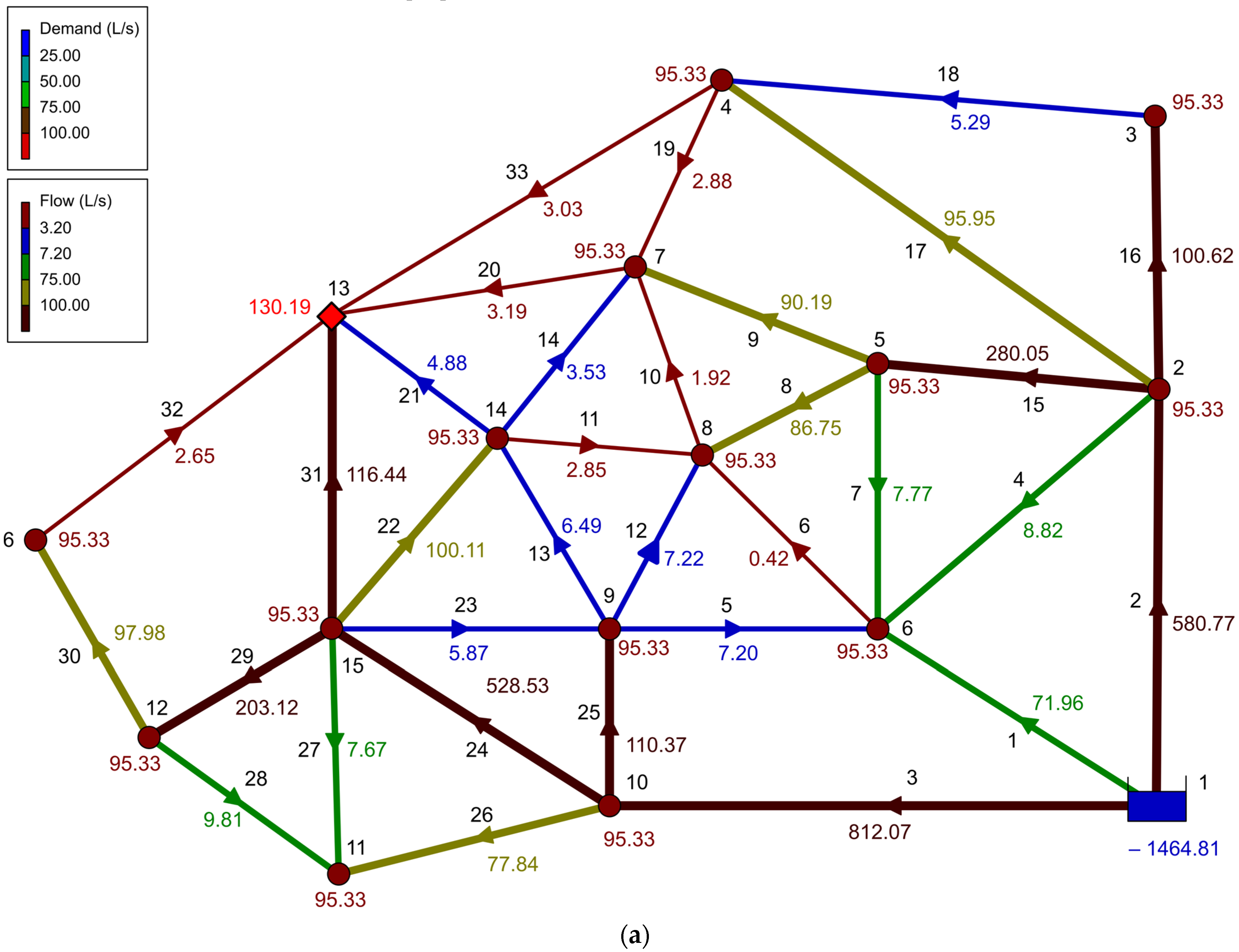
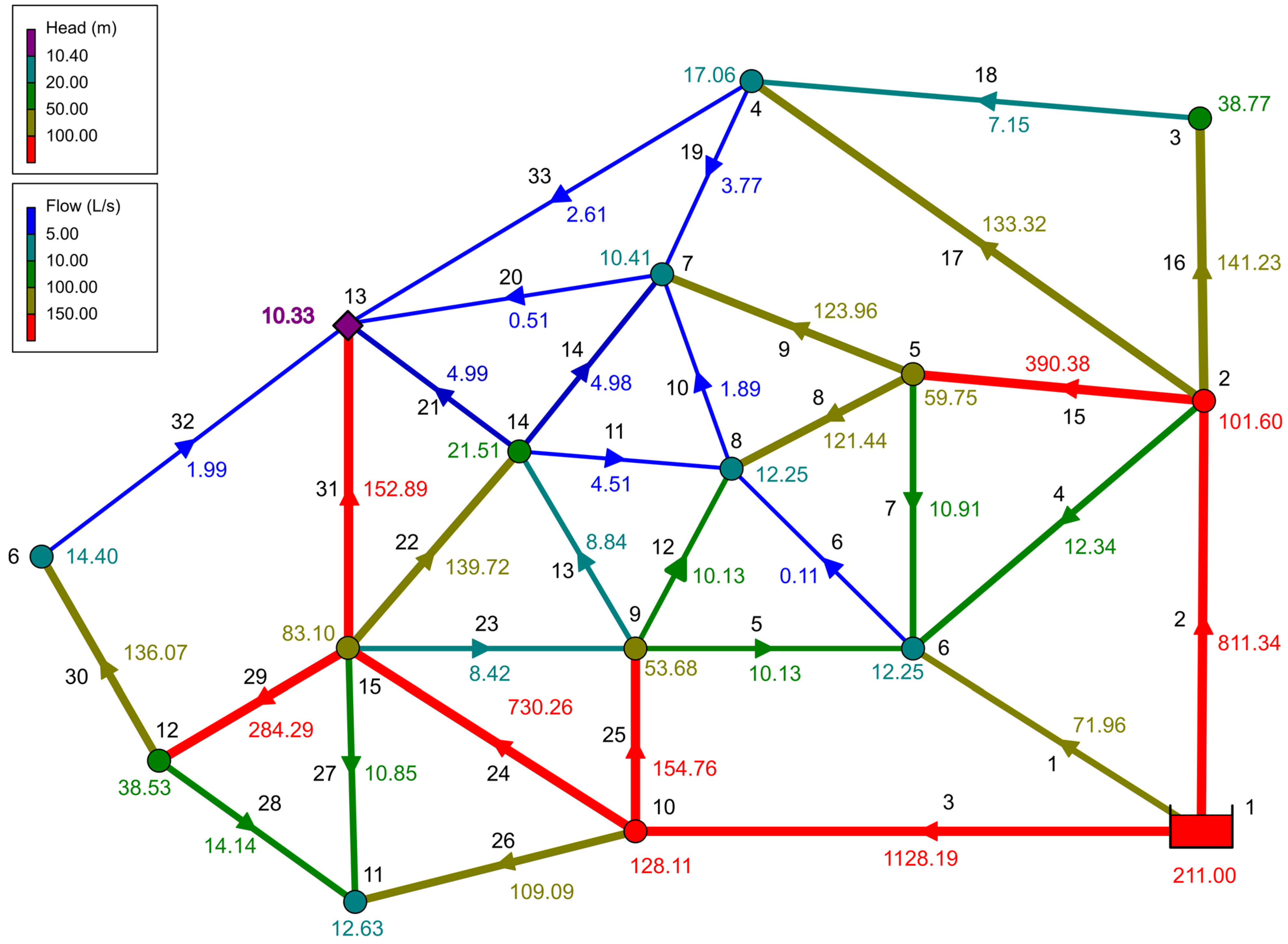
| Combination | A | Year: 2050 | Injection Height = | 211 | ||
| Qpeak + Qcc + Qcov40 + QPG + QF | FQ analys: | 3.055 + QF | ||||
| Network Table-Links | ||||||
| Demand | Pressure | Flow | Velocity | Unit Headloss | ||
| Node ID | L/s | m | Link ID | L/s | m/s | m/Km |
| Junc 2 | 134.08 | 101.60 | Pipe 2 | 811.34 | 4.13 | 29.89 |
| Junc 3 | 134.08 | 38.77 | Pipe 1 | 100.59 | 3.20 | 54.30 |
| Junc 4 | 134.08 | 17.06 | Pipe 3 | 1128.19 | 3.99 | 22.65 |
| Junc 5 | 134.08 | 59.75 | Pipe 4 | −12.34 | 1.57 | 32.61 |
| Junc 6 | 134.08 | 12.25 | Pipe 5 | −10.13 | 1.29 | 22.64 |
| Junc 7 | 134.08 | 10.41 | Pipe 6 | −0.11 | 0.01 | 0.00 |
| Junc 8 | 134.08 | 12.25 | Pipe 7 | −10.91 | 1.39 | 25.96 |
| Junc 9 | 134.08 | 53.68 | Pipe 8 | −121.44 | 2.47 | 25.96 |
| Junc 10 | 134.08 | 128.11 | Pipe 9 | 123.96 | 2.53 | 26.96 |
| Junc 11 | 134.08 | 12.63 | Pipe 10 | 1.89 | 0.24 | 1.01 |
| Junc 12 | 134.08 | 38.53 | Pipe 11 | −4.51 | 0.57 | 5.06 |
| Junc 13 | 163.01 | 10.33 | Pipe 12 | −10.13 | 1.29 | 22.64 |
| Junc 14 | 134.08 | 21.51 | Pipe 13 | 8.84 | 1.13 | 17.58 |
| Junc 15 | 134.08 | 83.10 | Pipe 14 | 4.98 | 0.63 | 6.07 |
| Junc 16 | 134.08 | 14.40 | Pipe 15 | −390.38 | 3.11 | 22.87 |
| Resvr 1 | −2040.13 | 211.00 | Pipe 16 | 141.23 | 2.88 | 34.33 |
| Pipe 17 | 133.32 | 2.72 | 30.85 | |||
| P min= | 10.33 | Junc 13 | Pipe 18 | 7.15 | 0.91 | 11.87 |
| P max= | 128.11 | Junc 10 | Pipe 19 | −3.77 | 0.48 | 3.63 |
| Pipe 20 | 0.51 | 0.07 | 0.04 | |||
| Pipe 21 | 4.99 | 0.64 | 6.11 | |||
| Pipe 22 | −139.72 | 2.85 | 33.66 | |||
| Pipe 23 | 8.42 | 1.07 | 16.07 | |||
| Pipe 24 | −730.26 | 3.72 | 24.60 | |||
| Pipe 25 | 154.76 | 3.15 | 40.67 | |||
| Pipe 26 | 109.09 | 3.47 | 63.10 | |||
| Pipe 27 | −10.85 | 1.38 | 25.72 | |||
| Pipe 28 | −14.14 | 1.15 | 14.15 | |||
| Pipe 29 | −284.29 | 2.95 | 24.36 | |||
| Pipe 30 | 136.07 | 1.93 | 13.18 | |||
| Pipe 31 | 152.89 | 3.11 | 39.77 | |||
| Pipe 32 | 1.99 | 0.25 | 1.11 | |||
| Pipe 33 | −2.61 | 0.33 | 1.84 | |||
Disclaimer/Publisher’s Note: The statements, opinions and data contained in all publications are solely those of the individual author(s) and contributor(s) and not of MDPI and/or the editor(s). MDPI and/or the editor(s) disclaim responsibility for any injury to people or property resulting from any ideas, methods, instructions or products referred to in the content. |
© 2024 by the authors. Licensee MDPI, Basel, Switzerland. This article is an open access article distributed under the terms and conditions of the Creative Commons Attribution (CC BY) license (https://creativecommons.org/licenses/by/4.0/).
Share and Cite
Benavides-Muñoz, H.M.; Lapo-Pauta, M.; Martínez-Solano, F.J.; Quiñones-Cuenca, M.; Quiñones-Cuenca, S. Global Events and Surge in Residential Water Demand: Exploring Possible Hydraulic Scenarios. Water 2024, 16, 956. https://doi.org/10.3390/w16070956
Benavides-Muñoz HM, Lapo-Pauta M, Martínez-Solano FJ, Quiñones-Cuenca M, Quiñones-Cuenca S. Global Events and Surge in Residential Water Demand: Exploring Possible Hydraulic Scenarios. Water. 2024; 16(7):956. https://doi.org/10.3390/w16070956
Chicago/Turabian StyleBenavides-Muñoz, Holger Manuel, Mireya Lapo-Pauta, Francisco Javier Martínez-Solano, Manuel Quiñones-Cuenca, and Santiago Quiñones-Cuenca. 2024. "Global Events and Surge in Residential Water Demand: Exploring Possible Hydraulic Scenarios" Water 16, no. 7: 956. https://doi.org/10.3390/w16070956