Article

Comparison of Methods Predicting Advance Time in Furrow Irrigation

1
Laboratory of Agricultural Hydraulics, Department of Natural Resources Development and Agricultural Engineering, Agricultural University of Athens, 11855 Athens, Greece
2
Laboratory of Mathematics and Theoretical Mechanics, Department of Natural Resources Development and Agricultural Engineering, Agricultural University of Athens, 11855 Athens, Greece
*
Author to whom correspondence should be addressed.
Water 2024, 16(8), 1105; https://doi.org/10.3390/w16081105
Submission received: 28 February 2024 / Revised: 4 April 2024 / Accepted: 10 April 2024 / Published: 12 April 2024
(This article belongs to the Special Issue Study of the Soil Water Movement in Irrigated Agriculture III)

Abstract

:
In the design of furrow irrigation, and in general in surface irrigation, the reliable estimation of the advance time at the furrow end (tL) is a key issue for improving the efficiency and uniformity of irrigation. In this study, three methods are used for estimating the tL, and their results are compared with the experimental data of fifteen different furrows from the international literature. These methods are as follows: (a) the Valiantzas equation, (b) the method presented by Walker and Skogerboe, based on solving the volume balance equation by the Newton–Raphson iterative procedure and (c) the method of Philip and Farrell. The first two methods assume that the infiltration is described by the Lewis–Kostiakov equation and the extended Lewis–Kostiakov equation, respectively, while in the case of the Philip and Farrell method, the infiltration is described by the Philip equation and the Lewis-Kostiakov equation. The results showed that in most cases of the first two methods, the absolute relative error value of the predicted time tL was less than 10%. The Philip and Farrell method using the Lewis–Kostiakov infiltration equation underestimates the time tL and fails especially in the case where the volume of the surface water is not negligible compared to the total volume of water entering the system. The Valiantzas method is recommended because it was simpler and easier to use and showed greater prediction accuracy of tL, resulting in better planning of irrigation systems and contributing to water saving, which is currently a big issue.

1. Introduction

The main characteristic of surface irrigation is the simultaneous advance and infiltration of water from the inlet to the end of a field. Part of the total water moves on the surface of dry soil as a thin surface layer, while at the same time the other part infiltrates into the soil when a soil surface comes into contact with water [1]. The shorter the advance time along the system, the greater the uniformity of the water depth infiltrating along the system [2]. However, this is very difficult to achieve, because the advance phase and in particular its completion time (tL) are affected by the water supply at the inlet of the system, the roughness coefficient, the longitudinal slope of the system and the infiltration rate.
In the design of surface irrigation systems, the accurate estimation of the time tL, i.e., the time that the advancing water front has reached the system end, plays a decisive role, because conventionally the irrigation time is usually taken as the sum of the time tL and the time that is required to infiltrate a water depth equal to the irrigation dose at the lower end of the field (ta). Thus, in the case where a water depth equal to the net irrigation dose (Zn) has been infiltrated at the lower end of the system, the degree of storage will be Es = 1 and the degree of efficiency Ea will be equal to E a = Z n L q o t δ , where q o is the inlet water rate, L is the furrow length and tδ is the total irrigation time, which is equal to t δ = t L + t a .
To predict the advance phase, several models have been proposed based on numerical solutions of surface flow models (e.g., kinematic wave model, zero inertia model, etc.) or the volume balance equation [3,4]. The zero-inertia model and the kinematic wave model have been found to reliably predict the advance phase in furrow irrigation [5,6,7]. However, the application of these models is not always easy, due to the complexity and difficulties related to the various numerical optimization techniques as well as the large number of their parameters. Such techniques are not easily adopted for routine furrow design applications.
Philip and Farrell [8] showed that by using the Laplace transformation, the general analytical solution of the Lewis and Milne [9] equation, which describes the infiltration–advance of water in surface irrigation when there is a constant inflow, can be obtained. Furthermore, by applying various infiltration equations, such as the Lewis–Kostiakov [10,11], Philip [12] and Horton [13] equations, into the general analytical solution, they obtained specific analytical solutions for the advance phase x(t) for each infiltration equation when the amount of surface water is considered negligible. However, in most cases, the infiltration equations used are empirical, and therefore their parameters have no physical meaning. In addition, the two-term infiltration equation of Philip [12] is only appropriate for infiltration at short to medium infiltration times [14].
The U.S. Soil Conservation Service (SCS) [15] has proposed an empirical equation to predict the duration of the advance phase, the application of which requires the classification of the soil in the appropriate permeability group.
Walker and Skogerboe [3], using the two-point volume balance equation and assuming that the advance phase is described by an exponential form equation, proposed an iterative procedure (Newton–Raphson method) to estimate the time tL from the furrow distance. Valiantzas [16] proposed algebraic equations to calculate the advance time as a function of inflow rate, without requiring iterative calculation procedures. A disadvantage of the method is perhaps that the time of advance versus distance relationship is described by three equations of different mathematical form [16].
Also, Valiantzas [17], based on the volume balance equation, proposed an equation to calculate the advance time as a function of the inflow rate and the parameters of the Lewis–Kostiakov infiltration equation, which gives similar results as the zero-inertia model. The equation was obtained by linear superposition of the two advance solutions for short times and the asymptotic solution for a longer time. This equation can also be applied to any form of the infiltration equation. Compared to the empirical SCS [14] equation, the Valiantzas [17] equation predicts the advance time much better.
Cook et al. [14] introduced into the Lewis and Milne [9] equation the two-parameter infiltration equation for linear soils presented by Philip [18]. This infiltration equation is based on physically meaningful parameters such as sorptivity (S) and saturated hydraulic conductivity (Ks) and is able to give adequate infiltration and advance behavior over all time scales.
From the abovementioned information, it appears that if we exclude the various simulation models of the duration of the advance phase, several analytical solutions and methodologies have been proposed that may be sufficient for routine furrow irrigation design applications. However, these solutions and their different methods rely on different assumptions and use different infiltration equations. However, a comparative evaluation of them, as far as we know, is absent from the literature.
The purpose of this paper is to compare (1) the Newton–Raphson iterative process proposed by Walker and Skogerboe [3], (2) the Valiantzas [17] equation and (3) the Philip and Farrell [8] method in predicting the advance time tL, as well as a comparison of their results with the experimental data from 15 experimental fields presented in the international literature. In the first two methods, it is assumed that the infiltration follows the Lewis–Kostiakov equation, while in the third method, both the infiltration equations described by Philip [12] and Lewis–Kostiakov are examined. The comparison of the three methods predicting the water advance in furrow irrigation could help irrigation system designers to choose the most suitable method each time. The choice of a reliable, easy and quick estimation of tL will help, among other things, to save water, which is currently a big issue.

2. Materials and Methods

2.1. Philip and Farrell Method [8]

The equation of Lewis and Milne [9] can describe the advance of water along a furrow as
q 0 t = c x + 0 x i t t s d s
where q0 (L3/T) is the constant inflow rate per furrow, c (L2) is the average section area of the stream flow, x (L) is the distance water has advanced along the field at time t, ts (T) is the value of t when water has arrived at location s behind the advancing front and i (L3/L) is the infiltration volume per unit length of furrow as a function of opportunity time t − ts.
An equivalent equation of (1) is Equation (2):
q 0 t = c x + 0 t i t t s x / t s d t s
where x / = d s d t s is the advance rate at time ts corresponding to location s.
Philip and Farrell [8] presented a solution of Equation (2) in series form, which gives the advance equation x(t) for short and long times via the Laplace transformation without assuming a functional form of x(t) before the integration of Equation (2).
If the Philip [12] equation (Equation (3)) is used as the infiltration equation
i t = S t 0.5 + A t ,
where S (L2/T0.5) is the soil sorptivity and A (L2/T) is related to saturated hydraulic conductivity Κs (L2/T) and varied 1/3 Κs < A < 2/3 Κs [18], then the solution of Equation [2] for c = 0 is
x t = q 0 A 1 e x p 4 A 2 t π S 2 e r f c 2 A t 0.5 π 0.5 S
According to Philip and Farrell [8], the case c = 0 is of particular interest because it shows in a simple way the dependence of x(t) on i(t) when the surface water volume relative to cumulative infiltration is small.
It should be noted that Equation (3) is valid for short to medium infiltration times [19]. Knowing the values of q, S and A of Equation (4), the value of tL can be calculated by using any generalized unconstrained technique in which f(tL) is minimized to zero. In this study, the tL was estimated using Excel Solver provided with Microsoft Excel 365 [20,21]. Excel Solver is an easy-to-use tool because it requires no programming knowledge.
More specifically, if Equation (4) is applied at the furrow distance x=L, where L is the furrow length, and the infiltration parameters A and S are known, then the only unknown parameter is the advance time t = tL. Equation (4) can be transformed into the following equation where the only unknown parameter is tL:
f t L = q 0 A 1 e 4 A 2 t L π S 2 e r f c 2 A t 0.5 π 0.5 S L = 0
The following steps were taken to solve Equation (5) and to estimate the tL by using the Solver tool:
Step 1:
Enter the values of the parameters q0, A, S and tL into an Excel worksheet. The value tL = 5A0L/q0 can be used as an initial value of tL, where A0 is the wetted cross-sectional area of a furrow.
Step 2:
In a new cell, calculate the f(tL) using Equation (5).
Step 3:
Go to the tools menu and click the Solver tool.
Step 4:
In “set objective”, set the cell created in step 2, then set it to receive the value zero according to Equation (5), and set the cell containing the value of tL as the Solver optimization variable. GRG nonlinear is chosen as the solution method.
Step 5:
Press OK and obtain an optimal value of tL.
Accordingly, if the infiltration equation used in Equation (2) is the Lewis–Kostiakov equation
i = k t α ,
where k (L2/Ta) and α (-) are empirical coefficients, then the following analytical solution for c = 0 is obtained:
x t = q 0 t 1 α k Γ 1 + α Γ 2 α
where Γ is the gamma function and k and α the parameters of the Lewis–Kostiakov equation. The calculation of time tL from Equation (7) is easier compared to Equation (4) since the calculation of tL can be performed explicitly from Equation (7) if the values of q0, k and α are known.

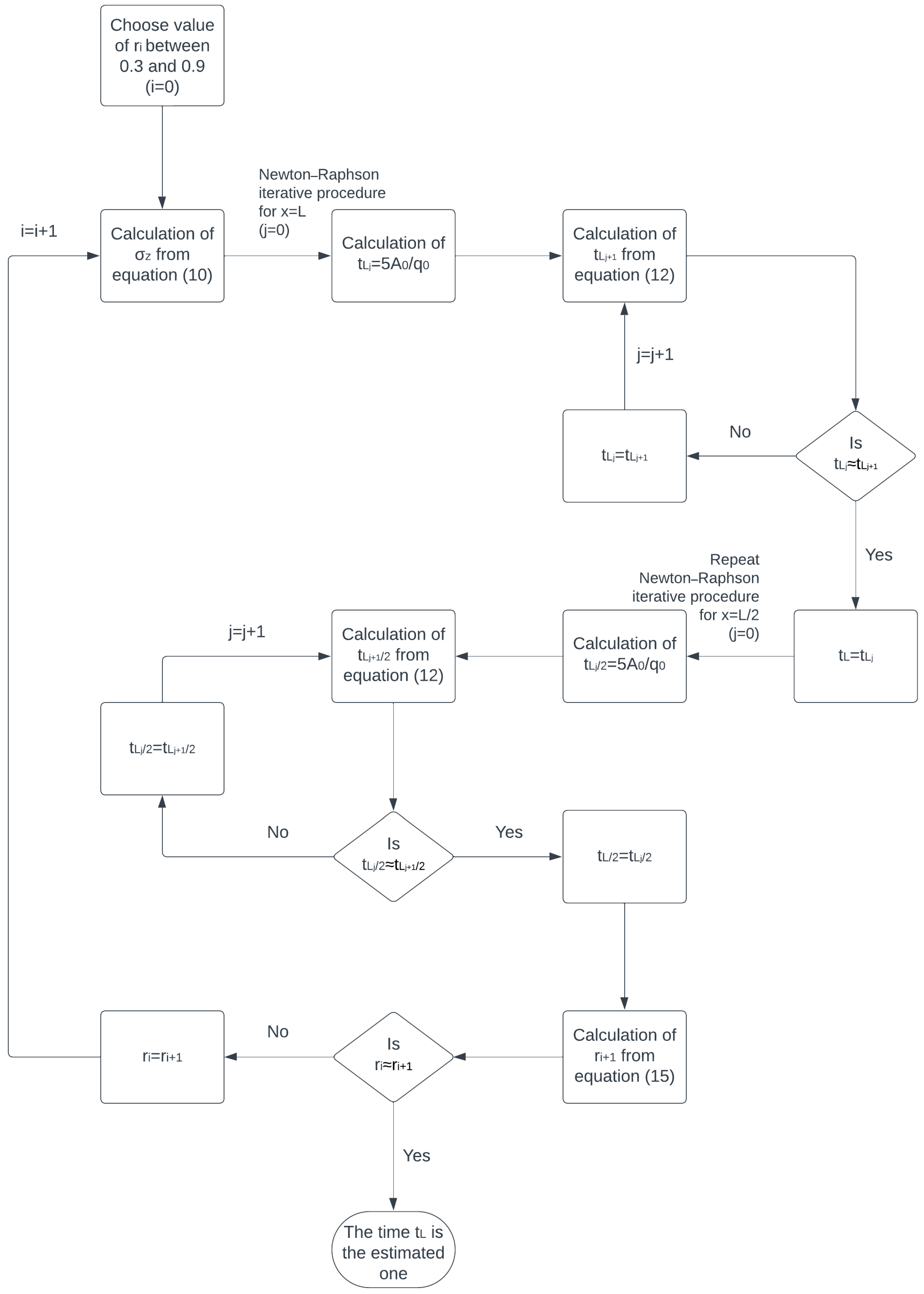
2.2. Newton–Raphson Iterative Procedure

The volume balance equation is based on the law of conservation of mass and was first applied by Lewis and Milne [9] (Equation (2)). It shows that the total volume of water at the inlet of the furrow at time t ≤ tL is expressed as q0t and is equal to the sum of the water volume flowing on the furrow surface and the water volume infiltrating into the soil according to the following relationship [3,22,23]:
q 0 t = σ y A 0 x + σ Z k t α x
where q0 (L3/T) is the inflow rate, x (L) is the distance of the advance water front at each time t (T), σy (-) is the surface profile shape factor, usually equal to 0.77 [24], σZ (-) is the subsurface shape factor, which ranges from 0.6 to 1, and the infiltration was assumed to follow the Lewis–Kostiakov equation, which is the most commonly used infiltration equation in surface irrigation models. A0 is the cross-sectional area of the inlet flow and is calculated from the Manning equation [3]:
A 0 = q 0 2 n 2 3600 ρ 1 S 0 1 ρ 2
where n (-) is the Manning roughness coefficient, ρ 1 and ρ 2 (-) are furrow shape parameters and S0 (-) is the longitudinal slope of the system (m/m).
Factor σZ is calculated by the following equation [25]:
σ Z = α + r 1 α + 1 1 + α 1 + r
where the advance curve is described by a power function of the form
x = p t r
where p and r are empirical adjustment coefficients. The introduction of this relationship over-conditions the problem by defining the advance relationship before the integration of Equation (2).
Equation (9) includes the furrow shape parameters ρ1 and ρ2, the advance distance x at time t, the longitudinal slope of the system (m/m) S0, the Manning roughness coefficient n, the inflow rate q0, the coefficients k and α of the Lewis–Kostiakov equation and the two unknown parameters tL and r. The parameter r is included in the calculation equation of the parameter σz (Equation (10)). Equation (8) can be solved using the Newton–Raphson iterative process to estimate the advance time tL, as well as the coefficient r. The steps followed are as follows:
(i)
First, an initial value of the parameter r is entered, which varies between 0.3 and 0.9. The value ri = 0.5 is usually chosen.
(ii)
Then, the value of the parameter σz is calculated, as mentioned in Equation (10). It should be noted that the value of σz is recalculated every time the value of r changes.
(iii)
The Newton–Raphson iterative procedure is then applied to find the advance time tL using the initial value ri as follows:
  • An initial estimate of tL0 is created. The value tL0 = 5A0L/q0 is usually considered as an initial value.
  • A better estimate of tL is tL1 given by the Newton–Raphson method using the relationship
    t L 1 = t L 0 f t L 0 f t L 0 = t L 0 c 1 t L 0 a + c 2 t L 0 + c 3 c 1 a t L 0 a 1 + c 2
    where
    f t L = c 1 t L a + c 2 t L + c 3 = 0
    and c1 = σZkL, c2 = −q0 and c3 = σyA0L.
  • Equation (13) is a transformed form of Equation (8) when x = L and t = tL. The initial estimate tL0 is compared with the value tL1. If the values tL0 and tL1 do not differ greatly, the next step, step 4 is applied; otherwise, step 2 is repeated and the tL2 value is calculated using tL1. The iterative process stops when two consecutive values converge. Empirically, three to four repetitions are sufficient.
  • The advance time at the distance x = L/2 is calculated accordingly for the initial value ri as described in steps 2 and 3, and the volume balance equation is applied by using the value L/2 instead of L.
(iv)
The value ri+1 is calculated using the advance times tL and tL/2 calculated from the previous steps 3 and 4 as follows:
r i + 1 = ln L L / 2 ln t L t L 2
or
r i + 1 = ln 2 ln t L t L / 2
(v)
The initial estimate ri is compared with the value ri+1 (Equation (15)). If the values converge, then it is assumed that the time tL is the estimated one. Otherwise, steps 2 to 4 are repeated using as a new initial value the value ri+1.
All the abovementioned steps of the Newton–Raphson iterative process can also be presented by the following flowchart (Figure 1).
It should be noted that if the inflow rate q0 in the furrow is too small and the length L is too long, then there is a failure to converge the values in the iterative process in step iii. In this case, when designing furrow irrigation, either q0 must be increased or the furrow length L must be reduced. Also, if the value of the coefficient r is known from some other method, then only steps ii and iii are applied to calculate tL.

2.3. Valiantzas Method [17]

The equation of Valiantzas [17] calculates, directly and algebraically, the advance time, as long as the inflow rate, the cross-sectional area of the inlet flow and the parameters k and α of the Lewis–Kostiakov equation of the corresponding soil are known (Equation (16)). Equation (16) was obtained by linear superposition of the solutions of the volume balance equation in dimensionless form for short and long times.
t L = 1 + 0.15 α A 0 L q 0 + σ Z F k L q 0 1 1 α
where k (L2/Ta) and α (-) are parameters of the Lewis–Kostiakov equation, A0 (L2) is the inlet flow area, L (L) is the length of the furrow, q0 (L3/T) is the inflow rate and σZF (-) is the value of parameter σZ (subsurface shape factor) at long times proposed by Hart et al. [26]:
σ Z F = α π 1 α sin α π
The first term on the right-hand side of Equation (16) reflects the volume of surface water, while the second term reflects the volume of infiltrated water. At short times, the first term is important, while at the long times the first term becomes negligible, and the second term dominates.
Valiantzas [17] reported that the maximum error in the estimation of time tL generally does not exceed ±7%, while in exceptional cases where the advance time is less than 30 min, the maximum error can exceed 10%.

2.4. Experimental Data

For the evaluation and comparison of the three methods, experimental data (data sets) from 15 different furrow irrigation experiments known from the international literature were used. More specifically, we used five series of experimental data derived from Walker and Busman [27], nine series from Wilson and Elliot [28] and one series from Camacho et al. [29]. The selected tests covered a wide range of soil infiltration parameters, inflow rates, furrow section shape parameters, field slopes and roughness coefficients. These data are presented in detail in Table 1. In all cases of experimental data, the authors present the parameters of k, α and f0 of the extended Lewis–Kostiakov infiltration function:
i = k t α + f 0 t
where f0 (L2/T) is the steady infiltration rate.
The k and α parameters of the Lewis–Kostiakov formula, which are used in the three methodologies, were estimated using the Solver tool in Excel (Table 2). Excel Solver minimizes the objective function between the measured (extended Lewis–Kostiakov infiltration function) and predicted cumulative infiltration values (Lewis–Kostiakov infiltration function) at given times and then predicts the k and α parameters of the Lewis–Kostiakov formula [30]. As the initial values of k and α parameters, we consider the values of the k and α parameters from the extended Lewis–Kostiakov infiltration function.
To calculate the sorptivity S and the parameter A of Equation (3) to be introduced as input parameters in Equation (4), first a check was conducted to see if the experimental infiltration data (extended Lewis–Kostiakov infiltration function) of all tests can be described by the Philip [12] infiltration equation. With a suitable transformation of the experimental data of each case, it was examined whether the relationship i/t0.5(t0.5) is linear. In this linear relationship, the slope of the line is equal to A and the constant term is equal to S [31]. From this analysis, it appeared that only in six cases the above relationship was linear. Then, for these six cases, the values of S and A were calculated using the Solver tool. As the initial values of S and A, we considered the values S = i1/t10.5 and A = (in − in−1)/(tn − tn−1), where n is the last value of the data. It should be noted that the values of S and A were almost the same with both the linearization method and the Excel Solver procedure.

3. Results and Discussion

Table 2 presents the values of the parameters k and α for all cases of furrows, which were calculated using Solver and are used to calculate the tL values in Equations (7) and (16), as well as in the iterative procedure. Also, Table 2 presents the values of the parameters S and A for six cases of data sets (i.e., Flowell wheel, Flowell non-wheel, Kimberly wheel, Kimberly non-wheel, Matchett M-1 and Printz P-1). In these data sets, the relationship i/t0.5(t0.5) is strongly linear, and the calculated values of S and A from Solver are positive. In the remaining cases, the relationship was not linear while the Solver calculated values A = 0, which have no physical meaning. Thus, the remaining cases were not studied further by applying Equation (4).
Table 3 presents the calculated values of coefficient r, which were obtained from the experimental data of the advance phase presented by Wilson and Elliot [28], Walker and Busman [27] and Camacho et al. [29] at two points of the furrows by applying Equation (11). Usually, the two experimental advance points are at the middle (L/2) and the end (L) of a furrow [32]. Thus, applying Equation (11) for two points, the following equations are obtained:
L = p t L r
L 2 = p t L 2 r
If Equations (19) and (20) are divided by terms and the logarithm of the resulting new equation is calculated, then the value of the parameter r is obtained as follows:
r = l n ( 2 ) l n t L t L 2
Additionally, Table 3 presents the values of the coefficient r calculated from the Newton–Raphson iterative procedure.
From the results presented in Table 3, it can be seen that the values of the coefficient r calculated by the iterative procedure converge with the values calculated from the experimental data using Equation (11). More specifically, the difference between the values of r does not exceed 7.5%, with the exception of the data from the Printz P-2 furrow, where the difference is 25.5%.
Table 4 shows the predicted values of tL from the three methods studied, as well as the measured values for all experimental furrows. The absolute values of relative errors (|RE|%) of the predicted values of tL with respect to the measured ones are presented in Table 5.
From Table 4 and Table 5, it can be seen that both the Valiantzas [17] method and the Newton–Raphson iterative procedure [3] satisfactorily approximate the measured values of tL in most cases. In more than half of the experimental furrows, the relative error is less than 10%, indicating that both methods predict the time tL fairly accurately. In general, the two methods converge on the tL value, and thus their deviation from the measured tL is approximately the same. The biggest differences in the two methods compared with the experimental data are observed in the Matchett data sets, where in all three cases (M1, M2 and M3) the RE values range from 11.96% to 25.81%. These deviations may be due to experimental errors related to inflow rate, roughness or furrow shape parameters. Possible problems with experimental measurements in these furrows were also reported by Valiantzas et al. [7].
Regarding the application of the Philip [12] method using the Lewis–Kostiakov infiltration equation in the data sets presented by Wilson and Elliot [28], Camacho et al. [29] and Walker and Busman [27] (Greeley Wheel data set), high RE values are shown, ranging from 18.19% to 59.24%, while in the remaining four data sets presented by Walker and Busman [27], the RE values are much smaller and closer to the values of the Valiantzas [17] method and the Newton–Raphson iterative procedure. In general, the method, in most cases, shows an underestimation of the time tL. To explain these findings, it was investigated whether the amount of surface water is negligible. For this purpose, the index Vs, which is equal to the ratio of the amount of surface water at the end of the advance phase to the total amount of water applied, was estimated in the 15 data sets.
V s = σ y A 0 x q 0 t L
The calculated Vs values showed that the surface water was 5.1%, 3.6%, 9.7% and 1.4% of the total application water for the Flowell wheel, Flowell non-wheel, Kimberly wheel and Kimberly non-wheel furrows, respectively. That is, the surface water amounts are very small, with the exception of the Kimberly wheel case (9.7%) where the corresponding RE value is 16.55%. In the rest of the data sets, the values of the Vs index are quite large and range from 7.1% to 40.9%. The highest RE values are observed in the cases of Greeley wheel and Cordoba, 59.24% and 51.59%, respectively, where the corresponding Vs index values are 0.409 and 0.355. It may be assumed that the same causes play a role in the failure of the Philip and Farrell [8] method in combination with the Philip [12] infiltration equation.
Figure 2 shows the relationships between the experimental values of time tL (tL,EXP) and the predicted ones (tL,PRED) for the three methods. As can be seen, these relationships are linear with a very high value of determination coefficient (R2 > 0.981). The Valiantzas [17] method gave the best results, since the slope of the linear relationship had the higher value (0.98), i.e., it is closer to the 1:1 line. In addition, it should be mentioned that this method is easy and simple to use, since the time tL is directly calculated from the furrow length L.
To obtain safer conclusions for the prediction of tL, RMSE (Root Mean Square Error) values for the three methods were also calculated. The RMSE values for the Valiantzas [17] and Newton–Raphson iterative procedure [3] methods were 22.14 min and 26.66 min, respectively, while for the Philip and Farrell [8] method in combination with the Lewis–Kostiakov equation the value was 43.19 min, which is almost twice the value of the other two methods.

4. Conclusions

To achieve maximum irrigation uniformity and efficiency in the design of surface irrigation systems and especially furrow irrigation, the reliable prediction of advance time tL is important. Especially currently, where water saving is a vital issue and the rational design of irrigation systems is required, the reliable and fast prediction of tL under various irrigation scenarios can help to optimize irrigation design.
In this context, a comparison of the three methods (Valiantzas [17] method, Newton–Raphson iterative procedure [3] and Philip and Farrell ([8D] method) was conducted to predict the completion time of the advance phase, tL, using experimental data of 15 different furrows from the international literature.
Among the three methods, the Valiantzas method was simpler and easier to use and showed greater prediction accuracy for experimental advance times from 45.5 to 560 min and for a wide range of values of the Lewis–Kostiakov equation parameters, i.e., under different soil types.
A similar performance was observed from the application of the volume balance equation in combination with the Newton–Raphson iterative procedure. Thus, this simple procedure can contribute to the design and evaluation of furrow irrigation systems. In most cases, the value of relative error for the Valiantzas method and the Newton–Raphson iterative procedure was less than 10%.
The Philip and Farrell method using the Kostiakov infiltration equation underestimated the time tL and failed especially in the case where the volume of surface water is not negligible. This is expected since the corresponding equation is obtained by considering the amount of surface water as negligible. These results can be very beneficial for irrigation system designers to study the irrigation performance of systems that are already working and to propose optimal solutions for each area.

Author Contributions

Conceptualization, G.K.; methodology, G.K., D.K., P.A.L. and L.M.; software, D.K. and L.M.; investigation, G.K., D.K., P.A.L. and L.M.; data curation, G.K., D.K., P.A.L. and L.M.; writing—review and editing, G.K., D.K., P.A.L. and L.M.; supervision, G.K. All authors have read and agreed to the published version of the manuscript.

Funding

This research received no external funding.

Data Availability Statement

Data are contained within the article.

Conflicts of Interest

The authors declare no conflicts of interest.

References

  1. Li, Y.; Bai, M.; Zhang, S.; Wu, C.; Li, F. Development In Improved Surface Irrigation in China. Irrig. Drain. 2020, 69, 48–60. [Google Scholar] [CrossRef]
  2. Or, D.; Silva, H.R. Prediction of Surface Irrigation Advance Trajectories Using Soil Intake Properties. Irrig. Sci. 1996, 16, 159–167. [Google Scholar] [CrossRef]
  3. Walker, W.R.; Skogerboe, G.V. Surface Irrigation: Theory and Practice; Prentice-Hall, Inc.: Englewood Cliffs, NJ, USA, 1987. [Google Scholar]
  4. Bautista, E.; Schlegel, J.L. WinSRFR 5.1—Software and User Manual; USDA-ARS Arid Land Agricultural Research Center: Maricopa, AZ, USA, 2019. [Google Scholar]
  5. Strelkoff, T.; Katopodes, N.D. Border-irrigation hydraulics with zero inertia. J. Irrig. Drain. Div. 1977, 103, 325–342. [Google Scholar] [CrossRef]
  6. Elliott, R.L.; Walker, W.R.; Skogerboe, G.V. Zero-inertia modeling of furrow irrigation advance. J. Irrig. Drain. Div. 1982, 108, 179–195. [Google Scholar] [CrossRef]
  7. Valiantzas, J.D.; Aggelides, S.; Sassalou, A. Furrow infiltration estimation from time to a single advance point. Agric. Water Manag. 2001, 52, 17–32. [Google Scholar] [CrossRef]
  8. Philip, J.R.; Farrell, D.A. General solution of the infiltration-advance problem in irrigation hydraulics. J. Geophys. Res. 1964, 69, 621–631. [Google Scholar] [CrossRef]
  9. Lewis, M.R.; Milne, W.E. Analysis of border irrigation. Agric. Eng. 1938, 19, 267–272. [Google Scholar]
  10. Kostiakov, A.N. On the dynamics of the coefficients of water percolation in soils and on the necessity of studying it from a dynamic point of view for purpose of amelioration. Trans. 6th Commun. Int. Soc. Soil Sci. Russ. Part A 1932, 17–21. Available online: https://cir.nii.ac.jp/crid/1520853835465008512 (accessed on 27 February 2024).
  11. Lewis, M.R. The rate of infiltration of water in irrigation practice. Trans. Am. Geophys. Union 1937, 18, 361–368. [Google Scholar] [CrossRef]
  12. Philip, J.R. The theory of infiltration: 4. Sorptivity and algebraic infiltration equations. Soil Sci. 1957, 84, 257–264. [Google Scholar] [CrossRef]
  13. Horton, R.E. An approach towards a physical interpretation of infiltration capacity. Soil Sci. Soc. Am. J. 1941, 5, 399–417. [Google Scholar] [CrossRef]
  14. Cook, F.J.; Knight, J.H.; Doble, R.C.; Raine, S.R. An improved solution for the infiltration advance problem in irrigation hydraulics. Irrig. Sci. 2013, 31, 1113–1123. [Google Scholar] [CrossRef]
  15. United States Department of Agriculture (USDA). Furrow Irrigation; Chapter 5, Section 15, Soil Conservation Service; USDA: Washington, DC, USA, 1983. [Google Scholar]
  16. Valiantzas, J.D. Explicit time of advance formula for furrow design. J. Irrig. Drain. Eng. 1999, 125, 19–25. [Google Scholar] [CrossRef]
  17. Valiantzas, J.D. Optimal furrow design. I: Time of advance equation. J. Irrig. Drain. Eng. 2001, 127, 201–208. [Google Scholar] [CrossRef]
  18. Philip, J.R. Theory of infiltration. Adv. Hydrosci. 1969, 5, 215–296. [Google Scholar]
  19. Parlange, J.-Y. Note on infiltration advance front from border irrigation. Water Resour. Res. 1973, 9, 1075–1078. [Google Scholar] [CrossRef]
  20. Mailapalli, D.R.; Wallender, W.; Raghuwanshi, N.; Singh, R. Quick method for estimating furrow infiltration. J. Irrig. Drain. Eng. 2008, 134, 788–795. [Google Scholar] [CrossRef]
  21. Rabbaniha, H.; Ebrahimian, H. Developing a simple method for estimating soil infiltration in furrow and border irrigation using advance, recession and runoff data. Irrig. Drain. 2024, 73, 50–63. [Google Scholar] [CrossRef]
  22. Elliott, R.L.; Walker, W.R. Field evaluation of furrow infiltration and advance functions. Trans. ASAE 1982, 25, 0396–0400. [Google Scholar] [CrossRef]
  23. Ebrahimian, H.; Ghaffari, P.; Ghameshlou, A.N.; Tabatabaei, S.-H.; Dizaj, A.A. Extensive comparison of various infiltration estimation methods for furrow irrigation under different field conditions. Agric. Water Manag. 2020, 230, 105960. [Google Scholar] [CrossRef]
  24. Bautista, E.; Clemmens, A.J.; Strelkoff, T.S. Structured application of the two-point method for the estimation of infiltration parameters in surface irrigation. J. Irrig. Drain. Eng. 2009, 135, 566–578. [Google Scholar] [CrossRef]
  25. Kiefer, F.W., Jr. Average Depth of Absorbed Water in Surface Irrigation; Special Publication; Department of Civil Engineering, Utah State University: Logan, UT, USA, 1965. [Google Scholar]
  26. Hart, W.E.; Bassett, D.L.; Strelkoff, T. Surface irrigation hydraulics-kinematics. J. Irrig. Drain. Div. 1968, 94, 419–440. [Google Scholar] [CrossRef]
  27. Walker, W.R.; Busman, J.D. Real time estimation of furrow infiltration. J. Irrig. Drain. Eng. 1990, 116, 299–318. [Google Scholar] [CrossRef]
  28. Wilson, B.N.; Elliott, R.L. Furrow advance using simple routing models. J. Irrig. Drain. Eng. 1988, 114, 104–117. [Google Scholar] [CrossRef]
  29. Camacho, E.; Perez-Lucena, C.; Roldan-Canas, J.; Alcaide, M. IPE: Model for management and control of furrow irrigation in real time. J. Irrig. Drain. Eng. 1997, 123, 264–269. [Google Scholar] [CrossRef]
  30. Kargas, G.; Koka, D.; Londra, P.A. Determination of Soil Hydraulic Properties from Infiltration Data Using Various Methods. Land 2022, 11, 779. [Google Scholar] [CrossRef]
  31. Smiles, D.E.; Knight, J.H. A note on the use of the Philip infiltration equation. Aust. J. Soil Res. 1976, 14, 103–108. [Google Scholar] [CrossRef]
  32. Panahi, A.; Seyedzadeh, A.; Maroufpoor, E. Investigating the midpoint of a two-point method for predicting advance and infiltration in surface irrigation. Irrig. Drain. 2021, 70, 1095–1106. [Google Scholar] [CrossRef]
Figure 1. Graphical overview (flowchart) of the steps of the Newton–Raphson iterative process.
Water 16 01105 g001
Figure 2. Comparative presentation between the measured values of advance time, tL,EXP, and the predicted ones, tL,PRED, obtained from the (a) Valiantzas method [17], (b) Newton–Raphson iterative procedure [3] and (c) Philip and Farrell [8] method using the Lewis–Kostiakov infiltration equation in all experimental furrows studied.
Water 16 01105 g002
Table 1. Furrow data.
Data SeriesWalker and Busman [27]Camacho et al. [29]
Flowell WheelFlowell Non-WheelKimberly WheelKimberly Non-WheelGreeley WheelCordoba
Inflow rateq0 (m3/min)0.120.120.090.0480.1140.09
Furrow slopeS0(m/m)0.0080.0080.01040.01040.0080.003
Manning roughness coefficientn0.040.040.040.040.040.04
Furrow shape parametersρ10.32690.32690.66440.66440.3690.39
ρ22.7342.7342.87872.87872.812.797
Furrow lengthL (m) = x2360274360112411200
Advance timetL (min) = t24004322085606351.5
Advance distance and corresponding timex1 (m)18014016060205.5100
t1 (min)4140481202620.25
Surface profile shape factorσy0.770.770.770.770.770.77
Extended Lewis–Kostiakov parametersα0.5340.6730.2120.5330.450.4550
k (m2/minα)0.00280.00220.00880.0070.00210.0033
f0 (m2/min)0.000220.000220.000170.000170.00000.0000
Data SeriesWilson and Elliot [28]
Benson B-1Benson B-2Benson B-3Matchett M-1Matchett M-2Matchett M-3Printz P-1Printz P-2Printz P-3
Inflow rateq0 (m3/min)0.16680.06840.07020.0510.05520.02640.28860.20940.1662
Furrow slopeS00.00440.00440.00440.00920.00950.00950.00230.00250.0025
Manning roughness coefficientn0.030.020.020.030.020.020.030.020.02
Furrow shape parametersρ10.460.580.340.31.352.120.920.6150.73
ρ22.862.912.842.7333.152.912.9242.98
Furrow lengthL (m) = x2500500500400400400200300300
Advance timetL (min) = t2175344.5247124.3232.221317845.573
Advance distance and corresponding timex1 (m)300300300200200200100100200
t1 (min)84.5159123.53870.588.213.51543
Surface profile shape factorσy0.770.770.770.770.770.770.770.770.77
Extended Lewis–Kostiakov parametersα0.020.020.010.480.40.160.40.020.02
k (m2/minα)0.02520.0180.01730.00110.00330.00390.00780.0130.0161
f0 (m2/min)0.000230.00010.000080.000030.000030.000020.001410.000490.0004
Table 2. Parameters of Lewis–Kostiakov equation (α and k) and Philip [12] equation (S and A) calculated with Solver tool.
ParametersWalker and Busman [27]Camacho et al. [29]
Flowell WheelFlowell Non-WheelKimberly WheelKimberly Non-WheelGreeley WheelCordoba
α0.75340.79160.51430.64580.45000.4550
k (m2/minα)0.00170.00180.00390.00500.00210.0033
S (m2/min0.5)0.0031050.0035470.0039160.007826--
A (m2/min)0.0002370.0003550.0000220.000205--
ParametersWilson and Elliot [28]
Benson B-1Benson B-2Benson B-3Matchett M-1Matchett M-2Matchett M-3Printz P-1Printz P-2Printz P-3
α0.35330.39520.27670.57200.47310.29660.7580.29290.3894
k (m2/minα)0.01030.00510.00770.00090.00270.00270.005760.01000.0083
S (m2/min0.5)---0.5720--0.006103--
A (m2/min)---0.000025--0.001296--
Table 3. Calculated values of coefficient r from Equation (11) and the Newton–Raphson iterative procedure [3].
Coefficient r
Experimental Furrows Equation (11)Newton–Raphson Iterative Procedure
Flowell wheel0.3040.354
Flowell non-wheel0.2820.297
Kimberly wheel0.5530.574
Kimberly non-wheel0.4050.382
Greeley Wheel0.7830.763
Cordoba0.7430.734
Benson B-10.7020.701
Benson B-20.6610.665
Benson B-30.7370.764
Matchett M-10.5850.606
Matchett M-20.5820.582
Matchett M-30.7860.749
Printz P-10.2690.309
Printz P-20.9900.735
Printz P-30.7660.691
Table 4. Measured and predicted values of advance time tL from the (a) Valiantzas method [17], (b) Newton–Raphson iterative procedure [3] and (c) Philip and Farrell [8] method using the Lewis–Kostiakov and Philip [12] infiltration equations in all experimental furrows studied.
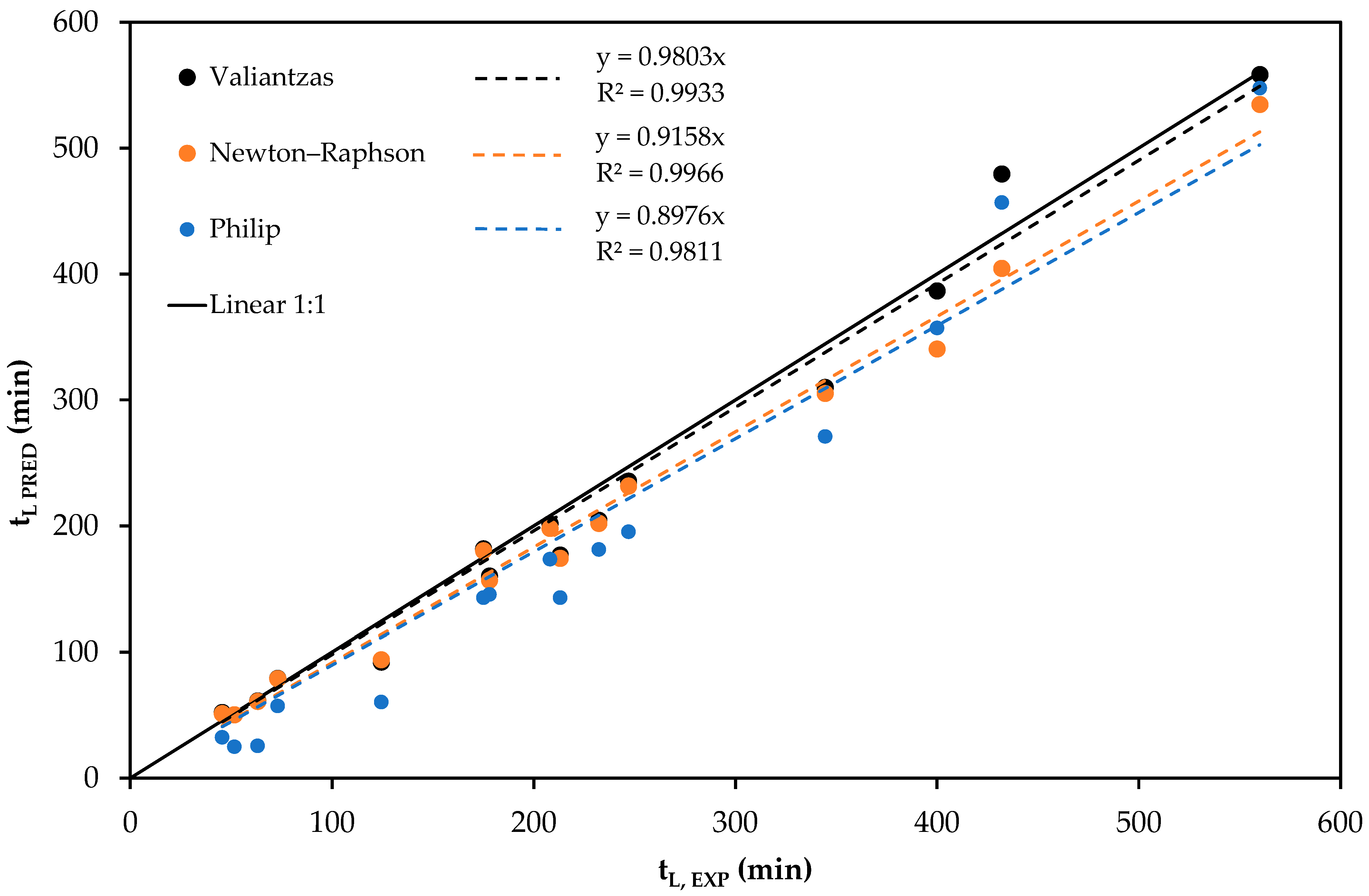
Advance Time tL (min)
Experimental FurrowsMeasured ValuesValiantzas Method Newton–Raphson
Iterative Procedure
Philip and Farrell Method
Lewis–Kostiakov EquationPhilip Equation
Flowell wheel400386.70340.53357.10397.80
Flowell non-wheel432479.51404.48456.86616.97
Kimberly wheel208201.87198.13173.57175.31
Kimberly non-wheel560558.46534.69547.60577.78
Greeley Wheel6361.4761.0425.67-
Cordoba51.550.3350.4024.93-
Benson B-1175181.86180.44143.07-
Benson B-2344.5310.00305.30271.13-
Benson B-3247235.54231.84195.37-
Matchett M-1124.392.2294.1160.4159.44
Matchett M-2232.2204.44202.08181.33-
Matchett M-3213176.85174.30143.13-
Printz P-1178160.31156.95145.62533.71
Printz P-245.552.2251.2532.53-
Printz P-37379.3579.0857.29-
Table 5. Absolute values of relative error (|RE|) between the measured and predicted values of advance time tL from the (a) Valiantzas method [17], (b) Newton-Raphson iterative procedure [3] and (c) Philip and Farrell [8] method using the Lewis–Kostiakov and Philip [12] infiltration equations in all experimental furrows studied.
|RE| (%)
Experimental FurrowsValiantzas MethodNewton–Raphson
Iterative Procedure
Philip and Farrell Method
Lewis–Kostiakov EquationPhilip Equation
Flowell wheel3.3314.8710.720.55
Flowell non-wheel11.006.375.7642.82
Kimberly wheel2.954.7416.5515.72
Kimberly non-wheel0.274.522.213.17
Greeley wheel2.423.1159.24-
Cordoba2.272.1351.59-
Benson B-13.923.1118.25-
Benson B-210.0111.3821.30-
Benson B-34.646.1420.90-
Matchett M-125.8124.2951.3930.83
Matchett M-211.9612.9721.91-
Matchett M-316.9718.1732.80-
Printz P-19.9411.8318.19199.84
Printz P-214.7612.6328.50-
Printz P-38.708.3321.51-
Disclaimer/Publisher’s Note: The statements, opinions and data contained in all publications are solely those of the individual author(s) and contributor(s) and not of MDPI and/or the editor(s). MDPI and/or the editor(s) disclaim responsibility for any injury to people or property resulting from any ideas, methods, instructions or products referred to in the content.

