Identifying and Interpreting Hydrological Model Structural Nonstationarity Using the Bayesian Model Averaging Method

Abstract

Understanding hydrological nonstationarity under climate change is important for runoff prediction and it enables more robust decisions. Regarding the multiple structural hypotheses, this study aims to identify and interpret hydrological structural nonstationarity using the Bayesian Model Averaging (BMA) method by (i) constructing a nonstationary model through the Bayesian weighted averaging of two lumped conceptual rainfall–runoff (RR) models (the Xinanjiang and GR4J model) with time-varying weights; and (ii) detecting the temporal variation in the optimized Bayesian weights under climate change conditions. By combining the BMA method with period partition and time sliding windows, the efficacy of adopting time-varying model structures is investigated over three basins located in the U.S. and Australia. The results show that (i) the nonstationary ensemble-averaged model with time-varying weights surpasses both individual models and the ensemble-averaged model with time-invariant weights, improving $NSE[\sqrt{Q}]$ from 0.04 to 0.15; (ii) the optimized weights of Xinanjiang model increase and that of GR4J declines with larger precipitation, and vice versa; (iii) the change in the optimized weights is proportional to that of precipitation under monotonic climate change, as otherwise the mechanism changes significantly. Overall, it is recommended to adopt nonstationary structures in hydrological modeling.

1. Introduction

Assessment of the hydrological response to climate change is an important research field [1,2]. Conventional impact evaluation usually involves the following steps: (1) modeling and predicting climate response under greenhouse gas emission scenarios using atmospheric circulation models (GCMs); (2) post processing/downscaling the output results of GCM; and (3) estimating the impact of climate change on a watershed scale based on hydrological models. Affected by climate characteristics on watershed and regional scales, uncertainties are introduced at every step in this top–down approach. Even the stress testing (or sensitivity-based) technique, which is independent from GCM results, can be affected by the uncertainties in hydrological model structures and parameters [3,4,5,6].

Developing reliable and robust hydrological models under climate change is a growing challenge in hydrological modeling [7]. Specifically, the extrapolative ability [8,9] of a model is particularly important when it is applied to scenarios outside the range of climate and hydrological characteristics in historical data used for parameter calibration [10]. The nonstationarity of hydrological models includes the nonstationarity of model parameters and model structural nonstationarity. The nonstationarity of model parameters is defined as a situation where model parameters vary in time [11]. Studies using Differential Split Sample Testing (DSST) have shown that model parameters do not remain consistent over time, but rather depend on the climate conditions in the calibration period [12,13,14]. Similarly, there is also nonstationarity in hydrological model structures. We defined the term “hydrological model structural nonstationarity” as the situation where the hydrological model structure varies in time, and thus the model’s relative performances depend on the period of the record used for modeling. Studies addressing model structural uncertainty have shown that it is impossible to identify a single optimal model for a specific watershed type, as relative performances among models vary over time [15,16,17,18].

Identification of and solution to catchment scale hydrological nonstationarity under climate change enables more robust decisions. The strategy of “multiple working hypotheses” has been widely applied in the research of hydrological model nonstationarity [19,20], including multiple parameter hypotheses and multiple structural hypotheses. There are two main ways to consider multiple model structures: (1) Flexible modular frameworks such as FUSE [15] and SUPERFLEX [21], for which studies have demonstrated that numerous hydrological models developed with varying structures and applicability are composed of universal and similar modules. These modular frameworks have universality and cover a wide range of model components, and therefore can be used to construct and analyze a larger and more diverse set of model structures under different climatic conditions. However, the accuracy and applicability of the restructured new model still need further verification. (2) Model ensemble averaging, such as Bayesian Model Averaging (BMA) [22], Akaike Information Criteria Averaging (AICA) [23], Granger-Ramanathan Averaging (GRA) [24], and the Arithmetic Averaging [25], etc., is also used. Compared with a single model, model ensemble averaging can overcome the potential lack of process representation, and therefore has better applicability when extrapolated to certain climatic and hydrological conditions [24,25,26,27,28]. Compared with flexible modular frameworks, the model ensemble averaging method is simpler to apply and is more efficient for hydrological modeling.

Post studies have investigated the best way of combining ensemble members and choosing averaging techniques under contrasting climatic conditions [29]. In traditional model ensemble averaging, fixed weights are usually adopted to runoff processes with different features [30]. Taking into consideration the strength of individual models for simulating different parts of runoff processes, studies modified the model ensemble averaging to adopt dynamic weights. Duan et al. [31] divided the runoff time series into several intervals due to magnitude and calculated BMA weights separately for each runoff interval. Rafter et al. [32] combined BMA with time sliding windows and calculated weights over each sliding window. Parrish et al. [33] and Xue and Zhang [34] combined BMA with Particle Filter and Ensemble Kalman Filter, respectively, and obtained daily updated weights. However, model ensemble averaging has seldom been applied in the study of model structural nonstationarity.

Considering that how to identify and interpret model structural nonstationarity has not been addressed in past studies, the objectives of this study are as follows: (i) propose a method to identify and quantify hydrological model structural nonstationarity by using the BMA Method; and (ii) reveal and interpret the mechanisms of hydrological model structural nonstationarity under climate change. It should be noted that the mechanism of model structural nonstationarity can be connected to multiple factors such as climate factors and the degree of climate change, the hydro-meteorological characteristics of catchment data, individual model structures, etc. Since it is difficult to consider all these factors together, this study concentrates on analyzing the correlation of precipitation change and model structural nonstationarity.

Regarding the multiple structural hypotheses, a method to identify the hydrological structural nonstationarity has been proposed by (i) constructing a nonstationary model through the Bayesian weighted averaging of two lumped conceptual rainfall–runoff (RR) models (the Xinanjiang and GR4J model) with time-varying weights; (ii) detecting and interpreting the temporal variation in the optimized Bayesian weights under climate change conditions. By combining the BMA method with period partition and time sliding windows, six modeling schemes are carried out and the efficacy of adopting time-varying model structures is investigated over three basins located in the U.S. and Australia. The remainder of this article is organized as follows: Section 2 describes the study site and materials used, and then presents a brief introduction to the methodology, including two RR models, the averaging techniques employed, and the six modeling schemes. Then, Section 3 presents the Results and Discussion. Finally, Conclusions are drawn in Section 4.

2. Materials and Methods

2.1. Study Site and Materials

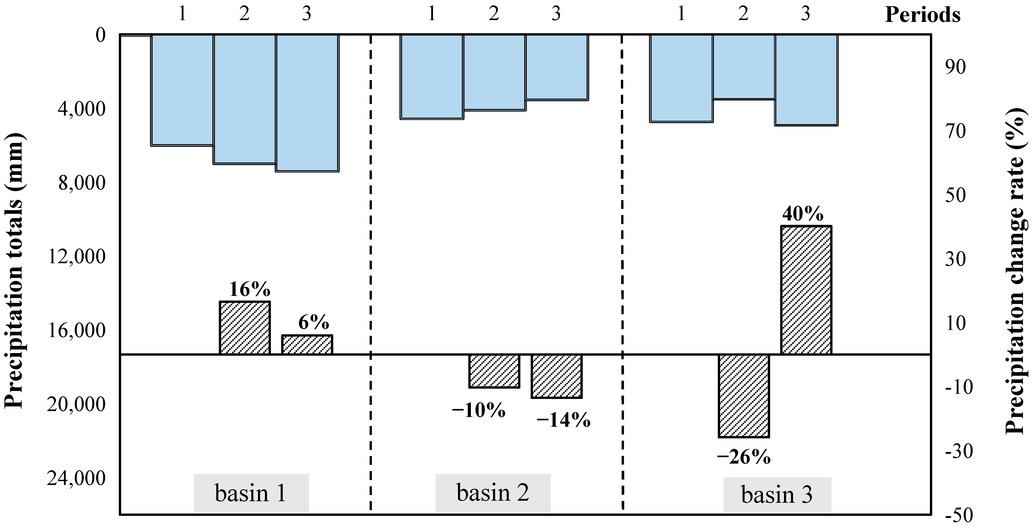
2.1.1. Study Site and Data Sources

The modeling experiments were conducted over three unimpaired basins with contrasting climate characteristics and varying degrees of climate change. Daily precipitation, climate potential evapotranspiration (ET_P), and runoff data were available for each basin, and the hydrometeorological characteristics and data sources of each basin are summarized in

Table 1. Hydrometeorological characteristics and data sources of the three study basins.

Data Source	Basin ID	Area (km2)	Runoff Coefficient	Mean Annual Rainfall (mm)	Mean Annual ETP (mm)	Mean Annual Runoff (mm)	Available Data Length	Period Partition
The MOPEX dataset in the U.S	basin 1	1002	0.40	1034	1065	407	1983–2003	The record of 1983–2003 is divided into three periods evenly: sub-period 1: 1983–1989 (7 years) sub-period 2: 1990–1996 (7 years) sub-period 3: 1997–2003 (7 years)
	basin 2	4828	0.06	619	1452	38
The national dataset of Australia	basin 3	990	0.46	613	1410	275	1970–2017 (1997–2009 is the period of millennium drought)	sub-period 1: 1990–1996 (7 years) sub-period 2: 2000–2006 (7 years, the millennium drought) sub-period 3: 2010–2016 (7 years)

. It can be seen that the selected basins cover an area of 990 to 4828 km² with the runoff coefficient varying from 0.06 (dry) to 0.46 (wet).

Basin 1 and basin 2 are from the Model Parameter Estimation Experiment (MOPEX) dataset in the United States [35]. As seen through a Mann–Kendall (MK) trend test of annual precipitation totals, the standard normal distribution statistics in both basins are above 1.96 with significance level α at 0.05, demonstrating that the climate (annual precipitation totals) change is significant.

Basin 3 is from the national dataset of Australia [36], which experienced a great decrease in runoff in the millennium drought from 1997 to 2009 [37,38]. Research has shown that the millennium drought in Australia resulted in changes to the rainfall–runoff relationship in a large number of basins [39].

To evaluate the temporal variation in precipitation totals, the data records for basin 1 and basin 2 are divided into three seven-year periods, evenly. For basin 3, to unify the length of the divided time periods, three seven-year periods are selected before, during, and after the millennium drought, respectively, as specified in Table 1. Figure 1 presents the precipitation totals and their change over three periods in the three study basins. It shows that basin 1 receives the maximum precipitation, and the precipitation totals increase steadily over three periods. Basin 2 receives less precipitation, and the precipitation totals decrease steadily over three periods. The precipitation totals in basin 3 decrease first for the millennium drought and then increase over periods, and the climate change degree is the largest among three basins, with the variation rates being higher than 25%.

2.1.2. Data Implementation

This study utilizes daily precipitation, ET_P, and runoff data in the study basins. Specifically, two-thirds of every period’s records are used for model calibration and the remaining for model validation. Data of the first 60 days in each period are sacrificed for model warming-up.

2.2. Methodology

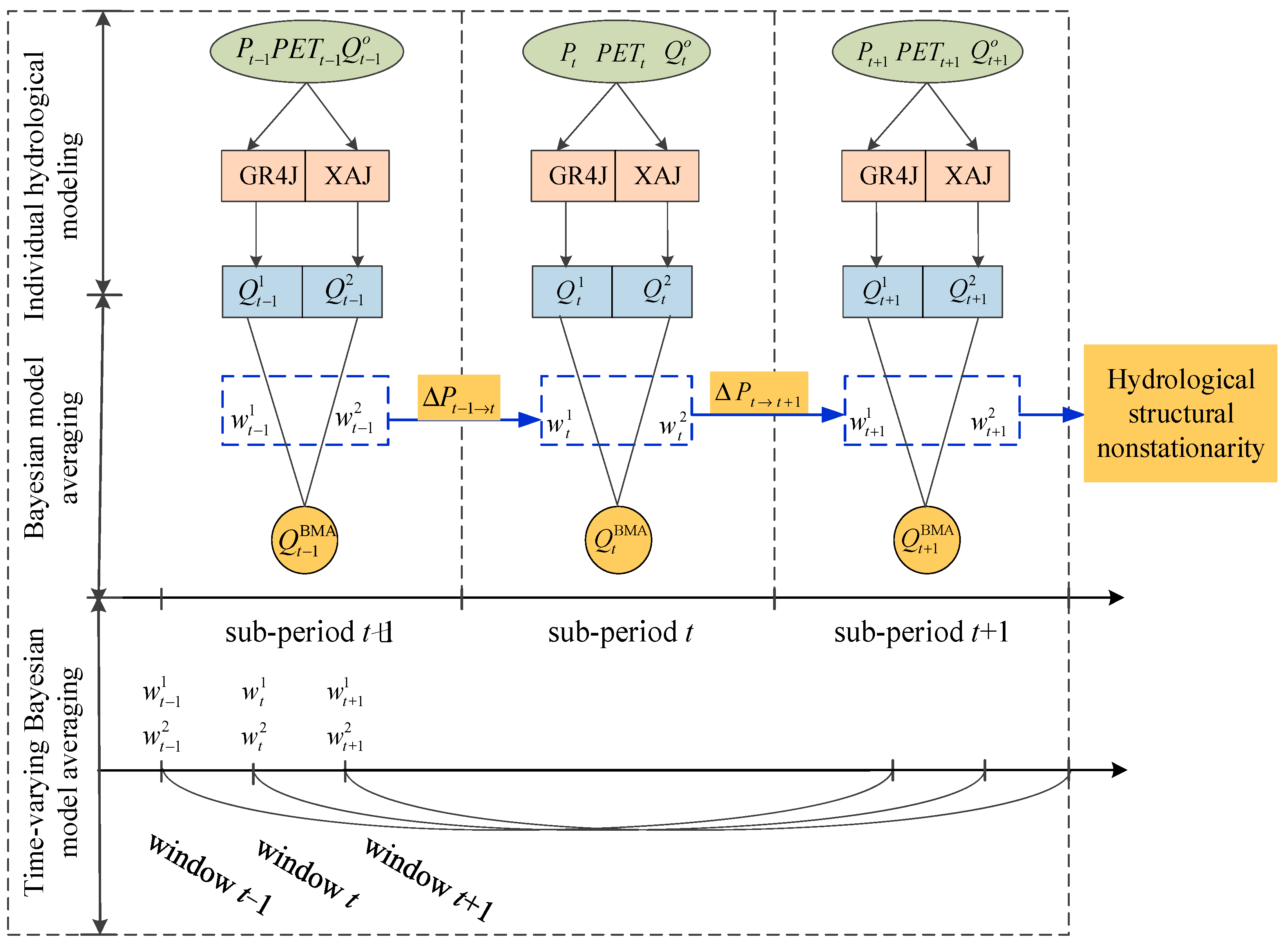
2.2.1. Overall Strategy of Nonstationarity Identification

The schematic diagram of the methodology is shown in Figure 2. Regarding the multiple structural hypotheses, the hydrological model structural nonstationarity is identified in three steps: firstly, hydrological modeling is conducted using the Xinanjiang and GR4J model individually; then, a nonstationary model structure is constructed through the Bayesian weighted averaging of the Xinanjiang and GR4J model; finally, the temporal variation in the optimized Bayesian weights is detected over different periods or time sliding windows under climate change conditions. By identifying the hydrological model structural nonstationarity, the efficacy of adopting time-varying model structures is investigated over three basins located in the U.S. and Australia.

2.2.2. Rainfall–Runoff (RR) Models

RR models in this study are selected on the basis of several criteria. Firstly, lumped conceptual RR models are required because they are widely used for hydrological nonstationarity research for relatively simple structures and few parameters. In addition, Fowler et al. [40] verified that conceptual RR models were more capable under changing climatic conditions than previously thought. Secondly, RR models are required to be representative (i.e., have different model structures, different numbers of parameters, and different emphases on physical processes) and widely used for runoff prediction over different climatic areas. Finally, it is expected that inputs to the RR models are daily precipitation and ET_P, considering the availability of data materials in this study. Considering the above factors, the Xinanjiang and GR4J model are selected for hydrological modeling and model averaging in this study.

The two models are contrasting in model structures (especially in the runoff production processes), parameter numbers, and applicability under different climatic conditions. Furthermore, both models have been demonstrated to produce favorable and comparable efficiency for runoff modeling through an experiment over 401 basins from the MOPEX [35].

(1)

Xinanjiang model

The Xinanjiang model is a conceptual lumped RR model developed in 1995 [41] and has been widely used for hydrological forecasts in humid and semi-humid regions [42]. The model structure consists of four main sub-modules and 15 parameters: (i) evapotranspiration (4-par: WUM, WLM, KE, C), (ii) runoff production (3-par: WM, B, IMP), (iii) runoff separation (4-par: SM, EX, KI, KG), and (iv) flow routing (4-par: CI, CG, N, NK). All the model parameters and their physical meanings are summarized in

Table 2. Parameters of the Xinanjiang and GR4J model and their physical meanings.

Model	Parameter	Physical Meaning	Range
Xinanjiang	B	Exponential of the distribution to tension water capacity	0.1–3
	SM	Areal mean free water storage capacity (mm)	1–80
	EX	Exponential of the distribution of free water storage capacity	0.7–2
	KI	Outflow coefficient of free water storage to the interflow	0.001–0.9
	KG	Outflow coefficient of free water storage to the groundwater	0.001–0.9
	IMP	Ratio of impervious area to the total area of the basin	0.0005–0.1
	C	Evapotranspiration coefficient of deep layer	0.1–0.25
	CI	Recession constant of the lower interflow storage	0.9–0.999
	CG	Recession constant of the lower groundwater storage	0.85–0.999
	N	Number of cascade linear reservoir of Nash model	0.1–10
	NK	Scale parameter of cascade linear reservoir	1–20
GR4J	x1	maximum capacity of the production store (mm)	50–1000
	x2	groundwater exchange coefficient (mm)	−10 to 10
	x3	one-day-ahead maximum capacity of the routing store (mm)	10–200
	x4	time base of unit hydrograph UH1 (days)	0.7–10

.

The main feature of the Xinanjiang model is the concept of runoff generation on the repletion of storage, which denotes that runoff is not produced until the soil moisture content of the aeration zone reaches field capacity. Thereafter, runoff equals rainfall excess without further loss, and the total runoff R is calculated using a soil moisture storage capacity distribution curve [41].

(2)

GR4J

GR4J is a 4-parameter lumped RR model, developed by Perrin based on the GR3J model [43,44], and has been successfully applied across a wide range of hydro-climatic conditions across the world [40,45]. The model structure comprises four main sub-modules: (i) determination of net rainfall/evapotranspiration capacity, (ii) production store, (iii) linear routing with unit hydrographs, and (iv) non-linear routing store. All the model parameters and their physical meanings are explained in Table 2.

The GR4J model is based on vertically-mixed runoff generation. In case the net rainfall P_n (the subtraction of evapotranspiration E from rainfall P) is not zero, a part P_s of P_n fills the production store and P_s is determined as a function of the level in the store. Then, a percolation leakage Perc from the production store is calculated as a power function of the reservoir content. Therefore, the total runoff P_r that reaches the routing functions is the sum of Perc and (P_n − P_s).

2.2.3. Model Calibration and Evaluation

(1)

Model calibration

It is of particular importance to simulate mean runoff in climate change impact studies [45]. The model parameters were calibrated to minimize the objective function F as Equation (1), which is the product of root-mean-square error (RMSE) and relative bias. The combination of these two terms is to minimize the simulation error of the discharge hydrographs as well as to ensure the overall water balance. To reduce the influence of high flows during calibration, square-root-transformed discharges are used to compute the RMSE.

$$\min F=\sqrt{\frac{1}{n}{\displaystyle \sum _{t=1}^n{(\sqrt{Q_{obs}(t)}-\sqrt{Q_{sim}(t)})}^2}}\times \left[1+\frac{\left|{\displaystyle \sum _{t=1}^n{Q}_{sim}}(t)-{\displaystyle \sum _{t=1}^n{Q}_{obs}(t)}\right|}{{\displaystyle \sum _{t=1}^n{Q}_{obs}(t)}}\right]$$

(1)

where $Q_{obs}(t)$ and $Q_{sim}(t)$ are the observed and simulated discharges on the tth day, respectively; n is the number of days.

Over different periods or time sliding windows, shown in Figure 2, the model parameters in Table 2 are estimated by successively using the genetic algorithm [46], Rosenbrock method [47], and the downhill simplex method [48]. These algorithms are able to converge on the near-optimal solution, and the combined application of these three algorithms merges the advantages of the respective methods, which is shown to be effective and computationally compact.

(2)

Model evaluation

Four indicators are used to evaluate the modeling performance: The Nash–Sutcliffe efficiency (NSE) [49], the Nash–Sutcliffe efficiency of square-root-transformed discharges ($NSE[\sqrt{Q}]$ or NSE_squrt), the root-mean-square error (RMSE), and the water balance index (WBI).

The indicator NSE, namely Equation (2), shows how well the residual variance matches the observed variance, and it indicates the extent to which observed and simulated variables follow the line with a 1:1 slope [50]. NSE is known to be biased toward higher flows. To provide a more balanced measure of performance across the hydrograph, $NSE[\sqrt{Q}]$ (NSE_squrt), calculated as Equation (3), is also used. Similarly, using square-root-transformed discharges reduces the influence of high flows, thus making it feasible to compare results among periods/basins of contrasted flow levels.

$$NS{E}_Q=\left[1-\frac{{\displaystyle \sum _{t=1}^n{(Q_{obs}(t)-Q_{sim}(t))}^2}}{{\displaystyle \sum _{t=1}^n{(Q_{obs}(t)-\overline{Q_{obs}})}^2}}\right]\times 100\%$$

(2)

$$NSE[\sqrt{Q}]=\left(1-\frac{{\displaystyle \sum _{t=1}^n{(\sqrt{Q_{sim}(t)}-\sqrt{Q_{obs}(t)})}^2}}{{\displaystyle \sum _{t=1}^n{(\sqrt{Q_{obs}(t)}-\overline{\sqrt{Q_{obs}}})}^2}}\right)\times 100\%$$

(3)

where $\overline{\sqrt{Q_{obs}}}$ is the average value of the square-root-transformed observed discharges.

RMSE indicates the averaged error between the simulated and observed streamflow, which is calculated as in Equation (4). A value of zero for RMSE means no bias, and smaller values indicate better performance.

$$RMSE=\sqrt{\frac{{\displaystyle \sum _{t=1}^n{\left[Q_{sim}(t)-Q_{obs}(t)\right]}^2}}{n}}$$

(4)

WBI indicates the relative volume error between the simulated and observed streamflow, which is calculated as in Equation (5). A value of zero for WBI means no bias, and a positive value indicates an overestimation of the total runoff volume and vice versa. Therefore, values closer to zero indicate better performance. Generally, a valve within $\pm$0.1 for WBI is favorable, but a value smaller than −0.2 or larger than 0.2 for WBI represents a significant hydrological bias.

$$WBI=\frac{{\displaystyle \sum _{t=1}^n{Q}_{sim}}(t)-{\displaystyle \sum _{t=1}^n{Q}_{obs}(t)}}{{\displaystyle \sum _{t=1}^n{Q}_{obs}(t)}}$$

(5)

2.2.4. Bayesian Model Averaging (BMA) Method

Bayesian Model Averaging (BMA) is a statistical procedure that infers probabilistic predictions by weighing individual model predictions [31,51]. The weights for individual models are based on their probabilistic likelihood measures, i.e., the posterior probabilities (the likelihood that an individual model is correct given the observations), with the better performing models receiving higher weights than the worse performing ones [52]. The prior distribution showed that all models have equal probabilities.

According to the law of total probability, the probability density function of the BMA prediction of discharge ($Q_{sim}$) can be expressed as

$$p(Q_{sim}|Q_{obs})={\displaystyle \sum _{k=1}^{K}p(M_k|Q_{obs})}·p(Q_{sim,k}|M_k,Q_{obs})$$

(6)

where $Q_{obs}$ is the observed discharge; $Q_{sim,k}$ is the simulated discharge of the individual model M_k; M = {M₁, M₂, …, M_K} is the ensemble set of individual models; $p(M_k|Q_{obs})$ denotes the posterior probability of model $M_k$ given the observed discharge $Q_{obs}$; $p(Q_{sim,k}|M_k,Q_{obs})$ denotes the posterior distribution of $Q_{sim}$ given the model M_k and the observed discharge $Q_{obs}$; k = 1, 2, …, K, K is the number of ensemble models. If we denote $w_k=p(M_k|Q_{obs})$ and ${\displaystyle \sum _{k=1}^K{w}_k}=1$, then the posterior mean of the BMA prediction is as follows:

$$E[Q_{sim}|Q_{obs}]={\displaystyle \sum _{k=1}^K{w}_k}·Q_{sim,k}$$

(7)

The Markov Chain Monte Carlo (MCMC) algorithm was applied to estimate the BMA parameters and then to calculate the optimal discharges.

In this study, Bayesian weighted averaging of the multi-model ensemble is regarded as constructing a new model structure, and the Bayesian weights represent the composition and dominance of the ensemble structures. Therefore, the structural nonstationarity of the new model under changing climate conditions can be detected from the temporal variation in the optimized Bayesian weights.

2.2.5. Modeling Schemes

To identify the hydrological model structural nonstationarity and investigate the efficacy of adopting time-varying model structures, six modeling schemes are implemented, as shown in

Table 3. Five modeling schemes implemented in this study.

Scheme	RR Model	Model Parameters	Bayesian Weights
1	individual XAJ model	fixed	/
2	individual GR4J model	fixed	/
3	time-invariant ensemble-averaged model	fixed	fixed
4	time-invariant ensemble-averaged model	time-segmented	fixed
5	time-varying ensemble-averaged model	time-segmented	time-segmented
6	time-varying ensemble-averaged model	time-sliding	time-sliding

.

(1)

Individual modeling schemes

Scheme 1 and Scheme 2 are the benchmark schemes, i.e., the conventional modeling schemes using the individual Xinanjiang and GR4J model, respectively, over the whole period.

(2)

Time-invariant model averaging schemes

Scheme 3 and Scheme 4 are two time-invariant model averaging schemes, with model averaging of the Xinanjiang and GR4J model with fixed Bayesian weights. In Scheme 3, model parameters are fixed over the whole period. Meanwhile, model parameters in Scheme 4 are calibrated over three different sub-periods and therefore time-segmented. These two schemes provide a second benchmark for model averaging.

For Scheme 4, the three sub-periods are divided as shown in Table 2.

(3)

Time-varying model averaging schemes

Scheme 5 and Scheme 6 are two time-varying model averaging schemes. Compared with time-invariant model averaging schemes, the estimation of Bayesian weights is based on an observation time series of a sub-period or a sliding window, instead of the whole calibration period. Therefore, the model structure can be adjusted according to observation and adapt better to climate change conditions.

The difference between these two schemes is the time step. In Scheme 5, the model parameters and Bayesian weights are evaluated over three different sub-periods and therefore time-segmented. The three sub-periods are divided as shown in Table 2. In Scheme 6, the BMA methods are combined with a time sliding window. Therefore, the model parameters and Bayesian weights are evaluated over different time sliding windows and therefore time sliding.

In Scheme 6, the size and interval width of time sliding windows are determined as 10 years and 1 year, respectively. On the one hand, the interval width of sliding windows cannot be two small to avoid auto-correlation in the observation time series. A past study of auto-correlation analysis on flow observation series found that the flow values were merely correlated with observation during the previous 40 days [33]. Therefore, an interval width of 1 year is adopted. On the other hand, larger window sizes correspond to a higher modeling efficiency and smaller uncertainties [33]. Thus, the window size is set as 10 years. Consequently, 12 time-sliding windows are generated from the 21-year datasets.

3. Results and Discussion

3.1. Streamflow Modeling Performances

Table 4. Streamflow modeling performances of six schemes in three study basins.

Basin ID	Evaluation Metrics	Modeling Schemes
		Scheme 1	Scheme 2	Scheme 3	Scheme 4	Scheme 5	Scheme 6
basin 1	NSE	0.83	0.78	0.84	0.86	0.87	0.89
	$NSE[\sqrt{Q}]$	0.61	0.6	0.64	0.69	0.71	0.75
	RMSE	25	21	17	13	7.7	5.4
	WBI	0.09	0.1	−0.07	0.05	0.05	−0.003
basin 2	NSE	0.42	0.53	0.54	0.55	0.56	0.58
	$NSE[\sqrt{Q}]$	0.51	0.58	0.59	0.6	0.61	0.63
	RMSE	10	9.5	6.2	4.8	4.1	2.5
	WBI	0.08	−0.06	0.05	−0.03	0.02	−0.001
basin 3	NSE	0.54	0.63	0.63	0.57	0.65	0.42
	$NSE[\sqrt{Q}]$	0.60	0.54	0.62	0.63	0.64	0.67
	RMSE	14	13	9.6	7.9	5.9	3.7
	WBI	0.12	−0.15	0.11	−0.08	0.10	−0.03

Note: the bold number indicates the best performance for each metric in a basin.

presents the streamflow modeling performances in three study basins (the best performance is bold). It can be seen that streamflow modeling efficiency is favorable in six schemes with an average NSE value of 0.65 and a maximum value of 0.89. The efficiency of mean runoff modeling is acceptable, with an average $NSE[\sqrt{Q}]$ value of 0.62 and a maximum value of 0.75. The water balance condition is generally satisfactory with an averaged WBI value within $\pm$0.1, guaranteeing the water balance for hydrological simulation. In addition, all schemes perform better in relatively wet basins (basin 1 and basin 3) than in arid regions (basin 2), showing the higher applicability of hydrological models under wet climate conditions.

Generally, the relative performance among the six modeling schemes is Scheme 6 > Scheme 5 > Scheme 4 > Scheme 3 >Scheme 2 > Scheme 1.

Compared with individual modeling schemes (Scheme 1 and Scheme 2), model averaging schemes (Scheme 3 to 6) are demonstrated to improve NSE values from 0.08 to 0.16, improve $NSE[\sqrt{Q}]$ values from 0.07 to 0.15, and reduce the absolute value of WBI by up to 0.097. The superiority of model averaging schemes under changes in climate can be explained by the fact that they can overcome the potential lack of process representation of an individual model.

The results of model averaging schemes demonstrate that using time-varying Bayesian weights can improve modeling performances under climate change conditions. Specifically, compared with time-invariant schemes (Scheme 5 and Scheme 6), time-varying schemes (Scheme 3 and Scheme 4) improve NSE values from 0.04 to 0.08, improve $NSE[\sqrt{Q}]$ values from 0.04 to 0.11, and reduce the absolute value of WBI by up to 0.08.

As for time-varying model averaging schemes, the ensemble-averaged model with time-sliding Bayesian weights (Scheme 6) surpasses that with time-segmented Bayesian weights (Scheme 5), in most cases with the $NSE[\sqrt{Q}]$ values improved from 0.02 to 0.04. The superiority of time-sliding windows is probably due to a smaller interval width and higher degree of flexibility, though the differences in efficiency are marginal between two schemes.

In general, compared with individual model structures, model ensemble averaging can overcome the potential lack of process representation of a single model, and thus it improves modeling performances in all cases. In addition, using time-varying model averaging can take into account model structural nonstationarity, and therefore it improves model adaptation and modeling performance under climate change.

3.2. Hydrological Model Structural Transferability Results

Based on the time-varying model averaging scheme with time-segmented Bayesian weights (Scheme 5), the structural transferability of the hydrological model is investigated by transferring the optimized Bayesian weights in each sub-period to the subsequent sub-periods for multi-model averaging.

Table 5. Streamflow modeling performances ($NSE[\sqrt{Q}]$) of the transferred model structure based on Scheme 5 in three study basins.

Basin ID	Periods	Modeling Schemes
		Xinanjiang	GR4J	BMA (Weights 1)	BMA (Weights 2)	BMA (Weights 3)
basin 1	sub-period 1	0.63	0.59	0.74	/	/
	sub-period 2	0.65	0.62	0.69	0.71	/
	sub-period 3	0.64	0.61	0.64	0.68	0.72
basin 2	sub-period 1	0.62	0.54	0.63	/	/
	sub-period 2	0.48	0.57	0.58	0.65	/
	sub-period 3	0.52	0.61	0.57	0.55	0.63
basin 3	sub-period 1	0.54	0.63	0.67	/	/
	sub-period 2	0.61	0.63	0.65	0.71	/
	sub-period 3	0.62	0.60	0.62	0.63	0.64

Note: BMA (weights 1), BMA (weights 2), and BMA (weights 3) are the BMA modeling schemes with the weights optimized in sub-period 1, sub-period 2, and sub-period 3, respectively. The bold number indicates the best performance over each sub-period in a basin.

presents the modeling performances ($NSE[\sqrt{Q}]$) of the transferred model structure based on Scheme 5 (the best performance is bold). The results show that in all cases, the BMA modeling scheme with the weights optimized in the original sub-period outperforms the scheme with weights transferred from other sub-periods, and the relative superiority of $NSE[\sqrt{Q}]$ can reach above 10%. In addition, the modeling efficiency is lower as the weights are transferred for a longer time interval, and even lower than that of an individual model. Specifically, in sub-period 2, the BMA modeling scheme with the weights optimized in sub-period 2 performs better than that with the weights optimized in sub-period 1. And, in sub-period 3, the BMA modeling scheme with the weights optimized in sub-period 3 performs the best, the scheme with the weights optimized in sub-period 2 worse, and the scheme with the weights optimized in sub-period 1 the worst.

The results demonstrate that transferring the hydrological model structure can decrease modeling efficiency, and the longer the time interval of transfer, the greater the decrease in efficiency. The structural transferability result of the hydrological model is similar to the transferability of hydrological model parameters [53].

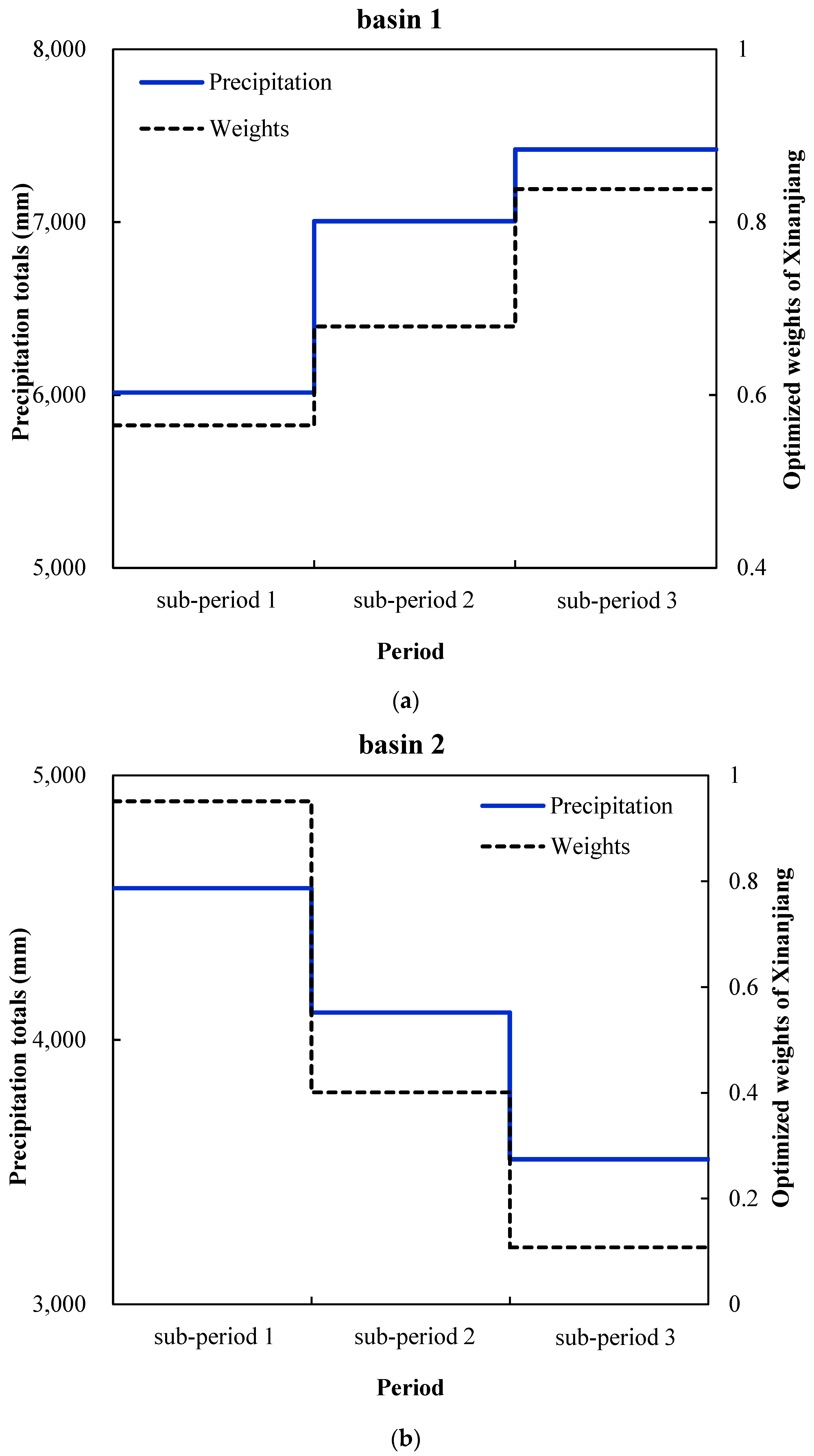
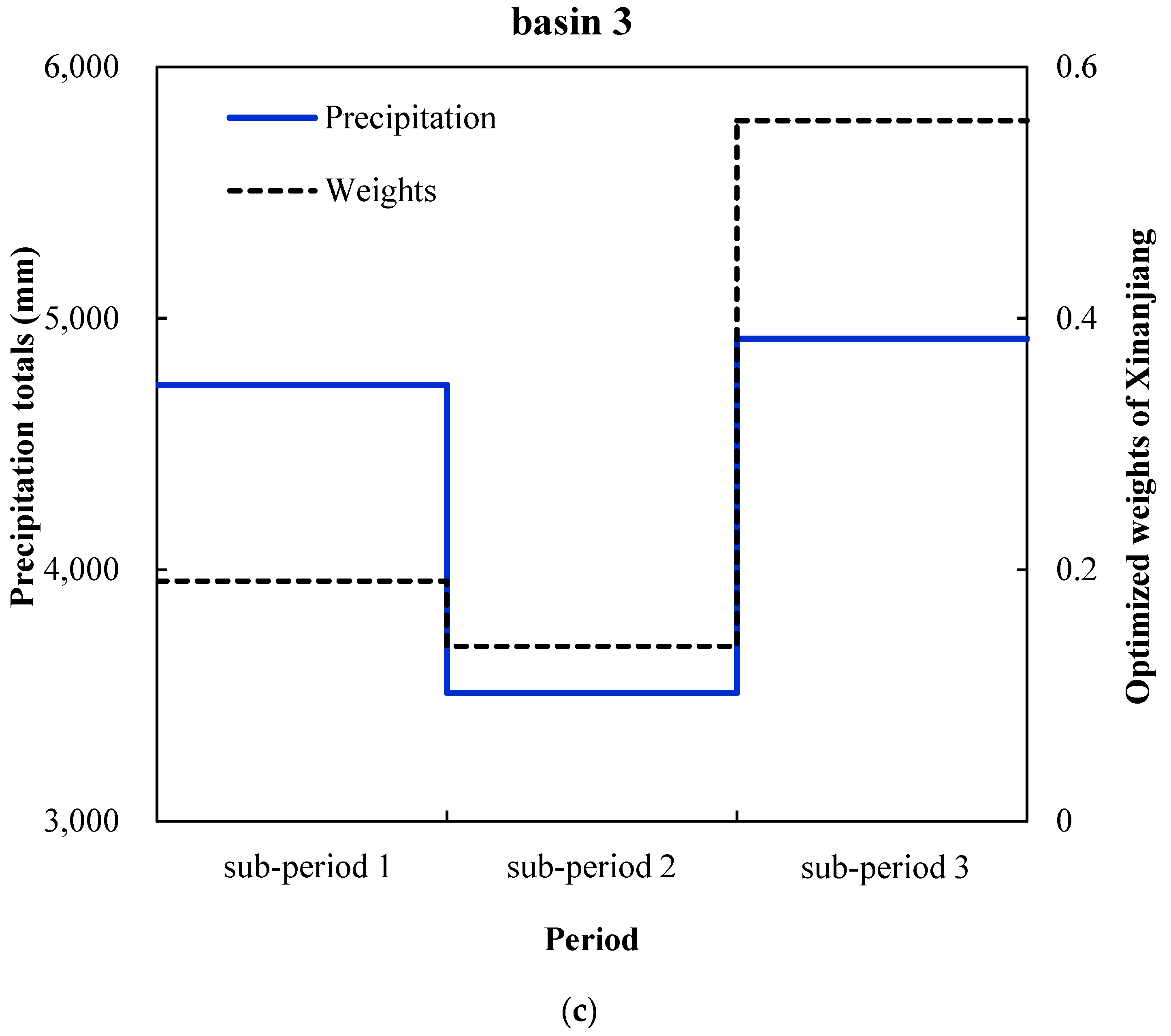
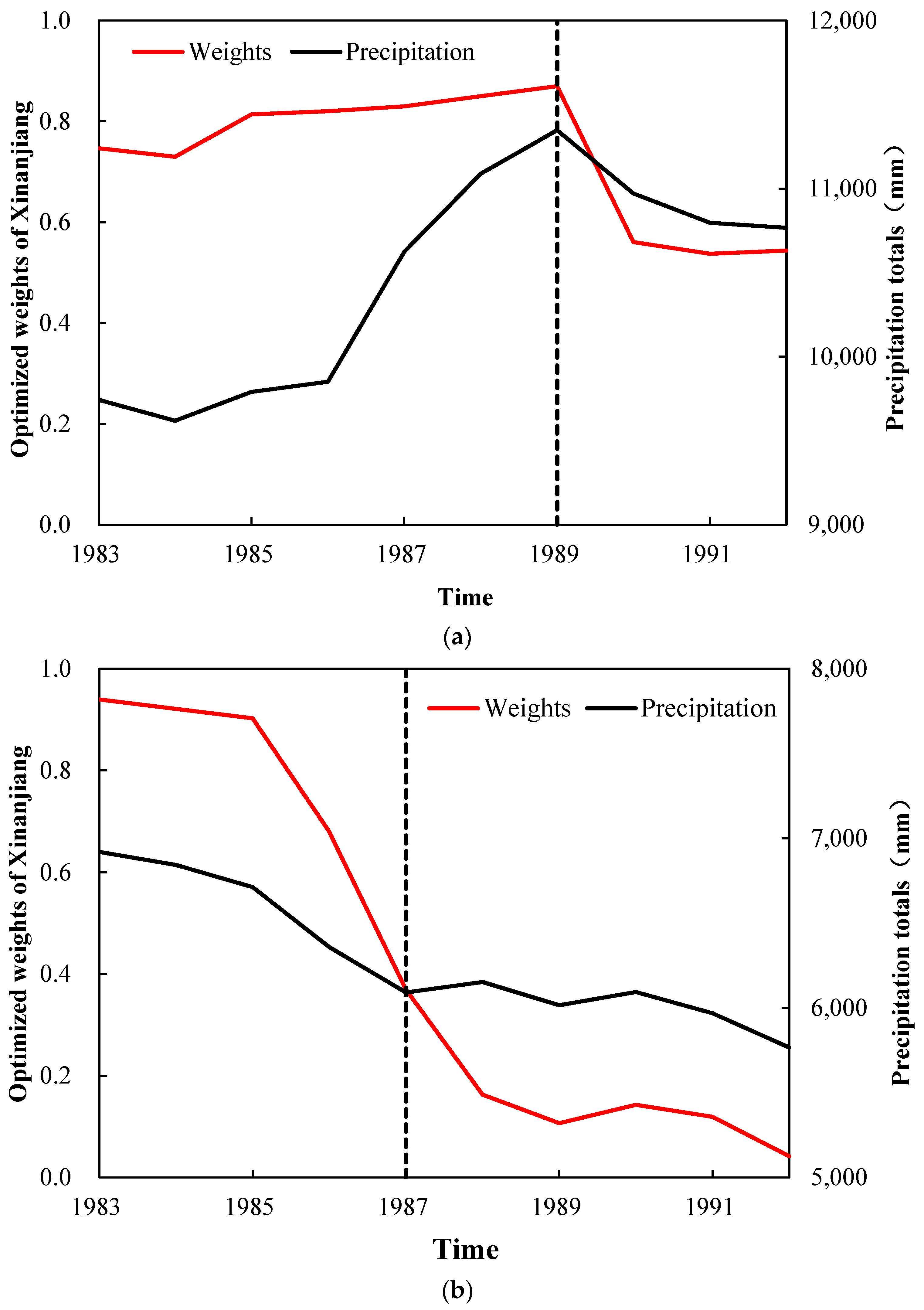
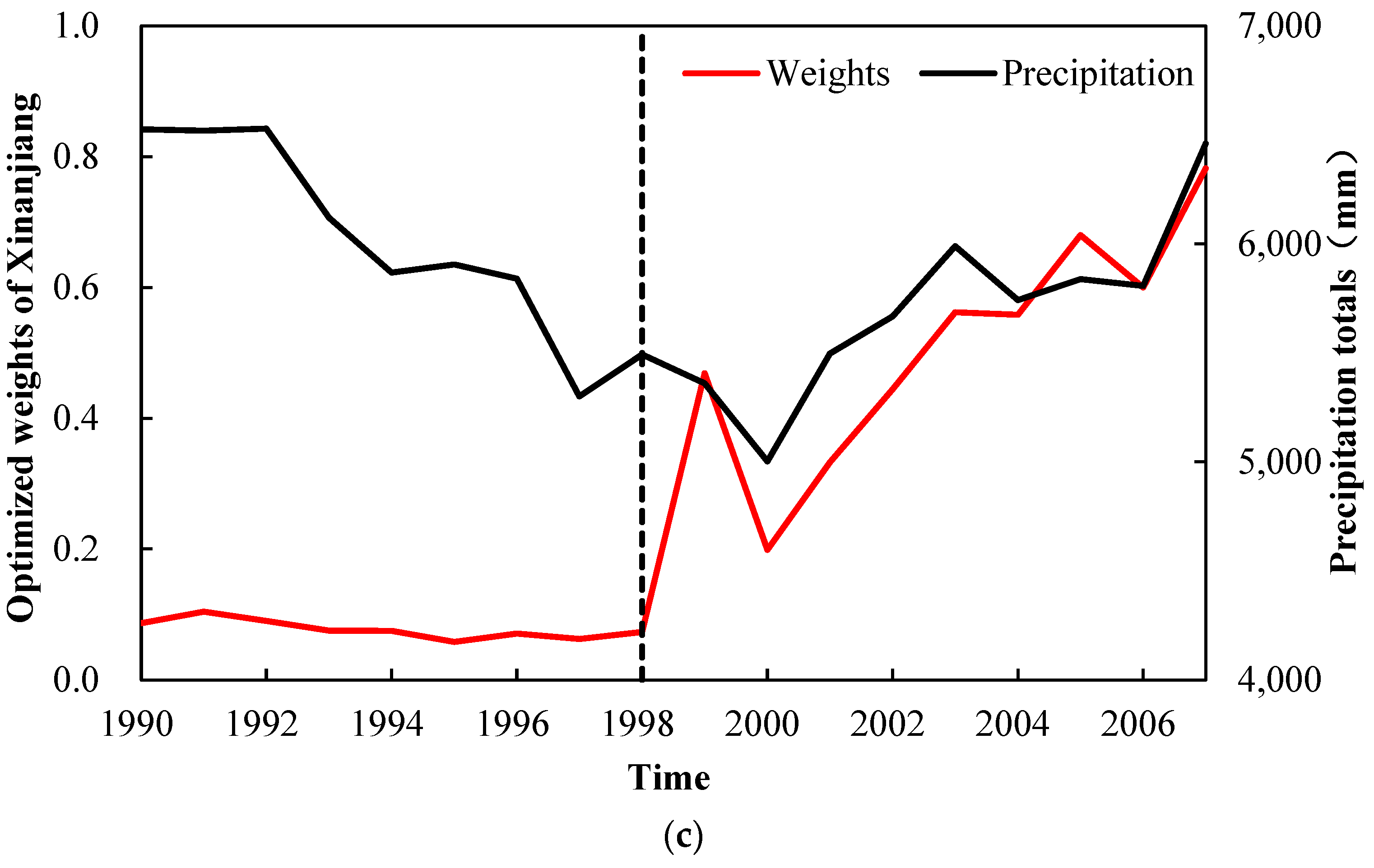
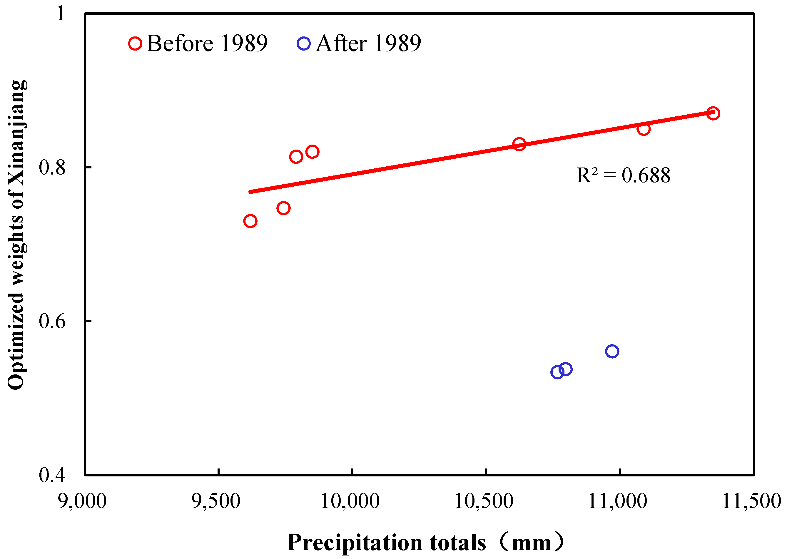
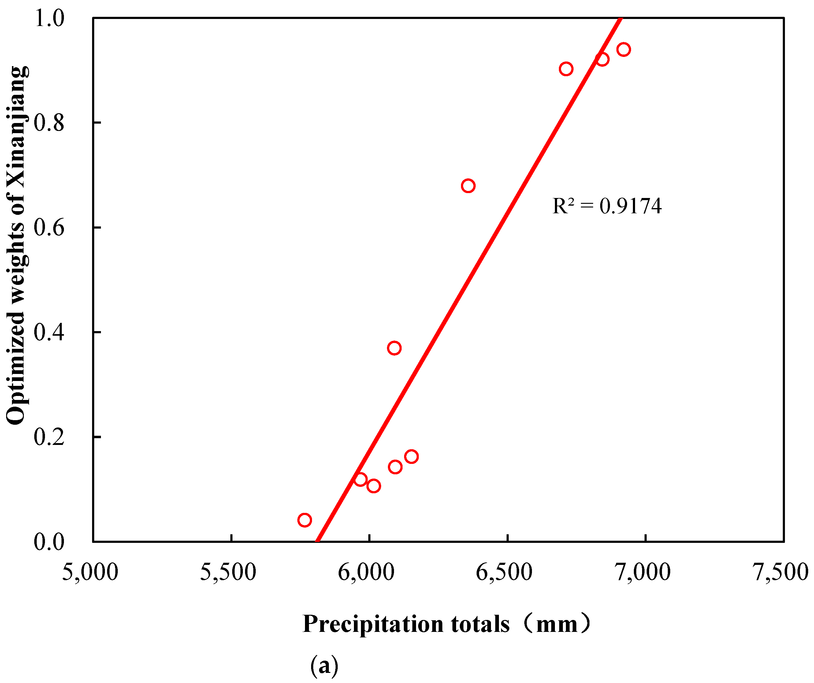
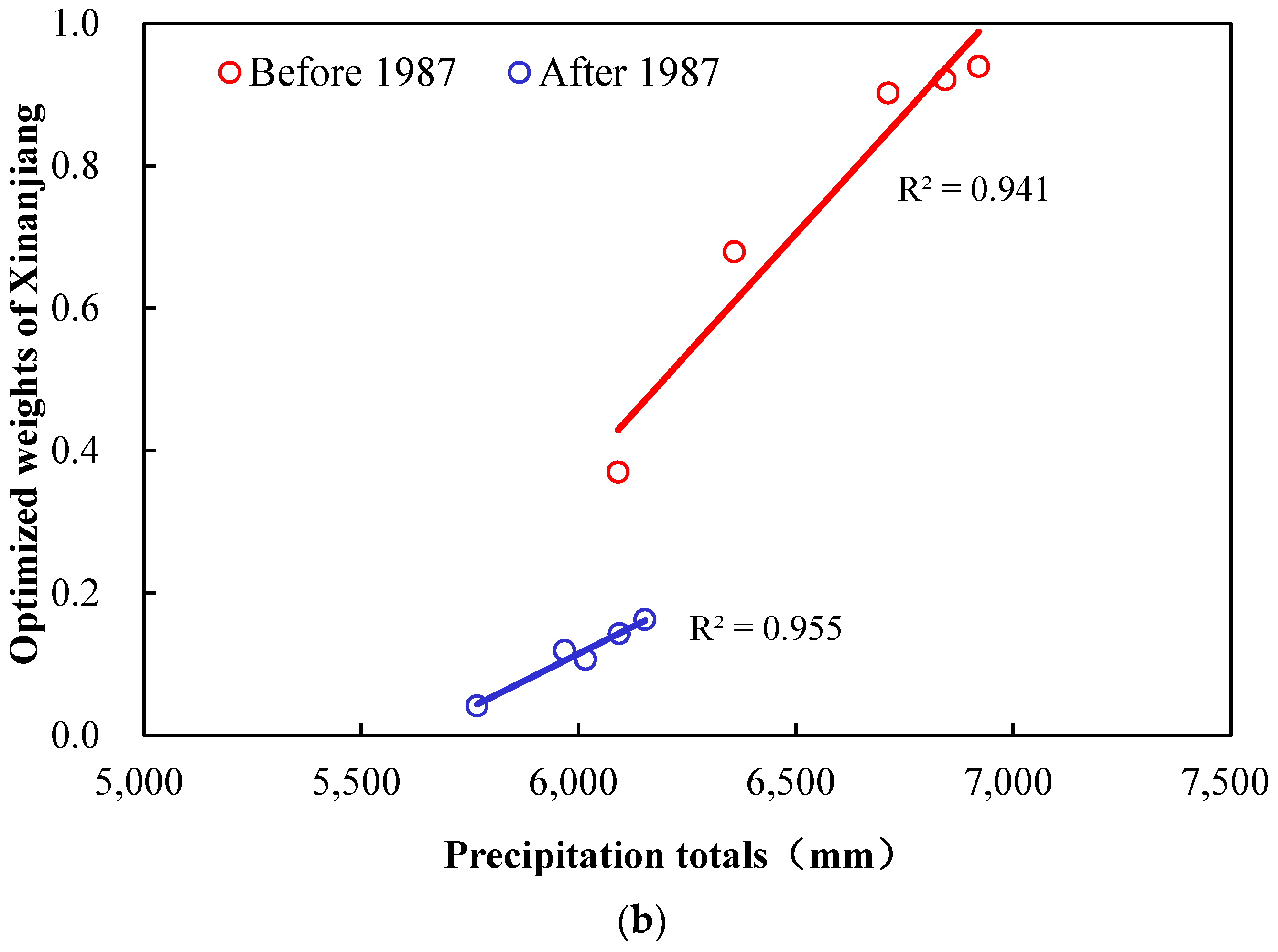
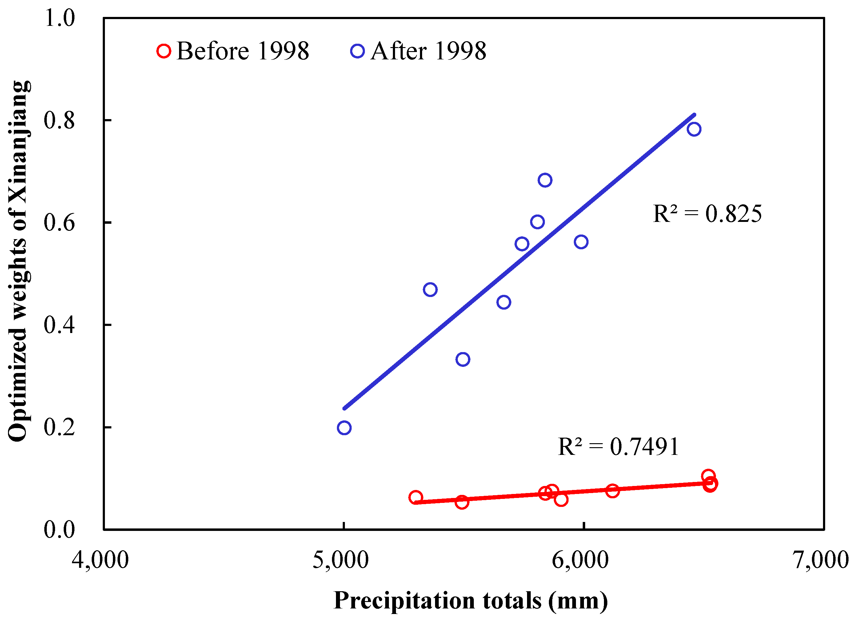
3.3. Identification of Hydrological Model Structural Nonstationarity

To identify the hydrological model structural nonstationarity, the temporal variation in the optimized Bayesian weights is detected over different sub-periods (based on Scheme 5) and time sliding windows (based on Scheme 6) under changing climate conditions. In all following results, the optimized weights of Xinanjiang model are analyzed, and the conclusion on the weights of GR4J is opposite and has not been presented.

Based on Scheme 5, by comparing the optimized weights with precipitation totals (mm) in each sub-period over three study basins (Figure 3), there is similar temporal variation in the precipitation values and weights of the Xinanjiang model.

Specifically, in basin 1, the optimized weights of the Xinanjiang model increase with precipitation increasing over all sub-periods, and the weights stay above 0.5. The results in basin 1 show that as the climate condition becomes wetter, the model structure is dominated by Xinanjiang, but the composition can vary under climate change.

In basin 2, the optimized weights of the Xinanjiang model decrease from above 0.5 to below 0.5 with a continuous reduction in precipitation. The results in basin 2 show that as the climate condition becomes drier, the model structure dominated by Xinanjiang is changed to be dominated by GR4J.

In basin 3, the precipitation experienced first a great decrease in the millennium drought and then a rebound during the last sub-period. Accordingly, the optimized weights of the Xinanjiang model decline and stay below 0.2 at first, and then increase to above 0.5. It can be inferred that in basin 3, the model structure dominated by GR4J is changed to be dominated by Xinanjiang.

Based on Scheme 6, Figure 4 presents the optimized weights of the Xinanjiang model and the precipitation totals (mm) in each time sliding window over three study basins. It can be seen that the optimized weights and precipitation change synchronously in the same direction.

Specifically, in basin 1, the climate condition is relatively wet with large precipitation totals and a runoff coefficient of 0.40. It can be seen that as the precipitation increases continuously before 1989, the optimized weights rise from 0.73 to 0.87. After 1989, the optimized weights of the Xinanjiang model decrease synchronously with the precipitation totals, but the model structure is dominated by the Xinanjiang model, with the optimized weights above 0.5 over the whole period.

In basin 2, the climate condition is relatively dry with medium precipitation totals and a runoff coefficient at 0.06. As the precipitation declines continuously, the optimized weights of the Xinanjiang model first drop from 0.92 to below 0.5 and then to 0.04. The hydrological model structure dominated by Xinanjiang has changed to be dominated by GR4J. Furthermore, it can be seen that the rate at which the weights decrease with precipitation declines has changed since 1987.

In basin 3, the climate condition is relatively wet with medium precipitation totals and a runoff coefficient of 0.46. Before 1989, the optimized weights of the Xinanjiang model dropped from 0.1 to 0.06 as the precipitation declined after the millennium drought. After 1989, the optimized weights rose to 0.78 as the precipitation increased. The hydrological model structure dominated by GR4J was changed to be dominated by Xinanjiang.

In all basins and different scenarios of climate change conditions, the temporal variation in the optimized Bayesian weights is consistent with that of precipitation, demonstrating the hydrological model’s structural nonstationarity under climate change.

3.4. Mechanisms of Hydrological Model Structural Nonstationarity

To further reveal the mechanisms of hydrological model structural nonstationarity under climate change, the correlation relationship between the optimized Bayesian weights and precipitation totals was investigated based on Scheme 6. In all the following results, the optimized weights of the Xinanjiang model are analyzed, and the conclusion about the weights of GR4J is consistent and has not been presented.

Figure 5 shows the optimized weights of the Xinanjiang model versus precipitation totals (mm) over different time sliding windows in basin 1. It can be seen that although there is a significant positive correlation between the two before 1989 (R² = 0.69), the correlation is demonstrated to be weak (R² < 0.5) over the period from the first year to any time after 1989 and even to be uncorrelated over the whole period (R² < 0.05). Therefore, the mechanism of hydrological model structural nonstationarity in basin 1 is revealed, i.e., a change in the optimized weights is directly proportional to a change in precipitation before 1989, and the mechanism of hydrological model structural nonstationarity has changed since 1989.

Figure 6 presents the optimized weights versus precipitation totals (mm) in basin 2. There is a significant positive correlation between the two over the whole period (R² = 0.92), before 1987 (R² = 0.94) and after 1987 (R² = 0.96). It can be inferred that a change in the optimized weights is directly proportional to a change in precipitation, but the change in the mechanism of hydrological model structural nonstationarity after 1987 is generally negligible.

Figure 7 shows the optimized weights versus precipitation totals (mm) in basin 3. It can be seen that the correlation is weak over the whole period (R² < 0.05); however, there is a significant positive correlation between the two before 1998 (R² = 0.83) and after 1998 (R² = 0.75). It reveals a similar mechanism of hydrological model structural nonstationarity in basin 3, i.e., a change in the optimized weights is directly proportional to a change in precipitation. In addition, the result indicates that the mechanism of hydrological model structural nonstationarity has changed significantly since 1998.

It is demonstrated in all basins and different scenarios of climate change conditions that the temporal variation in the optimized Bayesian weights is consistent with that of the precipitation, demonstrating the hydrological model’s structural nonstationarity under climate change. Furthermore, the mechanism of model structural nonstationarity has been revealed in that when the change in precipitation is monotonic (i.e., continuous increase or decrease), the correlation between the model structure and precipitation is monotonic linear [54,55]; when the change in precipitation is nonmonotonic (i.e., continuous increase followed by continuous decrease, or vice versa), the mechanism is altered significantly and results in a segmented linear correlation. The results can be explained by the irreversible changes in the watershed’s hydrological characteristics [56,57,58].

4. Conclusions

Understanding catchment-scale hydrological nonstationarity under climate change enables managers to make more robust decisions. Regarding the multiple structural hypotheses, this study aims to propose a method to identify hydrological structural nonstationarity using the BMA method. By combining the BMA method with period partition and time sliding windows, the efficacy of adopting time-varying model structures is investigated over three basins located in the U.S. and Australia. By comparing and analyzing the results, conclusions and implications are drawn as follows:

(i)

Using time-varying model structures can take into account the model’s structural nonstationarity, and therefore it improves model adaptation and modeling efficiency under climate change.

(ii)

Transferring the hydrological model structure can decrease modeling efficiency, and the longer the time interval of transfer, the greater the decrease in efficiency.

(iii)

The temporal variation in the optimized Bayesian weights is consistent with that of precipitation.

(iv)

Furthermore, when the change in precipitation is monotonic, there is a change in the optimized weights proportionally; when the change in precipitation is nonmonotonic, the mechanism of hydrological model structural nonstationarity changes significantly and results in a segmented correlation between the model structure and precipitation.

Overall, hydrological model structural nonstationarity can be identified under change and adopting nonstationary structures in hydrological modeling is recommended. It should be noted that modeling performance is also related to the degree of climate changes and the physical processes of model structure; thus, the mechanism of model structural nonstationarity needs further research.

References

1. Dolgorsuren, S.E.; Ishgaldan, B.; Myagmartseren, P.; Kumar, P.; Meraj, G.; Singh, S.K.; Kanga, S.; Almazroui, M. Hydrological Responses to Climate Change and Land-Use Dynamics in Central Asia’s Semi-arid Regions: An SWAT Model Analysis of the Tuul River Basin. Earth Syst. Environ. 2024. [Google Scholar] [CrossRef]
2. Peiris, T.A.; Doell, P. Improving the quantification of climate change hazards by hydrological models: A simple ensemble approach for considering the uncertain effect of vegetation response to climate change on potential evapotranspiration. Hydrol. Earth Syst. Sci. 2023, 27, 3663–3686. [Google Scholar] [CrossRef]
3. Prudhomme, C.; Wilby, R.L.; Crooks, S.; Kay, A.L.; Reynard, N.S. Scenario-neutral approach to climate change impact studies: Application to flood risk. J. Hydrol. 2010, 390, 198–209. [Google Scholar] [CrossRef]
4. Prudhomme, C.; Sauquet, E.; Watts, G. Low flow response surfaces for drought decision support: A case study from the UK. J. Extrem. Events 2015, 2, 1550005. [Google Scholar] [CrossRef]
5. Whateley, S.; Steinschneider, S.; Brown, C. A climate change range-based method for estimating robustness for water resources supply. Water Resour. Res. 2014, 50, 8944–8961. [Google Scholar] [CrossRef]
6. Wilby, R.L.; Dawson, C.W.; Murphy, C.; Connor, P.O.; Hawkin, E. The Statistical DownScaling Model—Decision Centric (SDSM-DC): Conceptual basis and applications. Clim. Res. 2014, 61, 259–276. [Google Scholar] [CrossRef]
7. Klemeš, V. Operational testing of hydrological simulation models. Hydrol. Sci. J. 1986, 31, 13–24. [Google Scholar] [CrossRef]
8. Anderson, M.P.; Woessner, W.W. The role of the postaudit in model validation. Adv. Water Resour. 1992, 15, 167–173. [Google Scholar] [CrossRef]
9. Oreskes, N.; Shrader-Frechette, K.; Belitz, K. Verification, validation and confirmation of numerical models in the earth sciences. Science 1994, 263, 641–646. [Google Scholar] [CrossRef] [PubMed]
10. Milly, P.C.D.; Betancourt, J.; Falkenmark, M.; Hirsch, R.M.; Kundzewicz, Z.W.; Lettenmaier, D.P.; Stouffer, R.J. Climate change—Stationarity is dead: Whither water management? Science 2008, 319, 573–574. [Google Scholar] [CrossRef] [PubMed]
11. Westra, S.; Thyer, M.; Leonard, M.; Kavetski, D.; Lambert, M. A strategy for diagnosing and interpreting hydrological model nonstationarity. Water Resour. Res. 2014, 50, 5090–5113. [Google Scholar] [CrossRef]
12. Wagener, T.; McIntyre, N.R.; Lees, M.J.; Wheater, H.S.; Gupta, H.V. Towards reduced uncertainty in conceptual rainfall-runoff modelling: Dynamic identifiability analysis. Hydrol. Process. 2003, 17, 455–476. [Google Scholar] [CrossRef]
13. Choi, H.T.; Beven, K. Multi-period and multi-criteria model conditioning to reduce prediction uncertainty in an application of TOPMODEL within the GLUE framework. J. Hydrol. 2007, 332, 316–336. [Google Scholar] [CrossRef]
14. Herman, J.D.; Reed, P.M.; Wagener, T. Time-varying sensitivity analysis clarifies the effects of watershed model formulation on model behavior. Water Resour. Res. 2013, 49, 1400–1414. [Google Scholar] [CrossRef]
15. Clark, M.P.; Slater, A.G.; Rupp, D.E.; Woods, R.A.; Vrugt, J.A.; Gupta, H.V.; Wagener, T.; Hay, L.E. Framework for Understanding Structural Errors (FUSE): A modular framework to diagnose differences between hydrological models. Water Resour. Res. 2008, 44, W2B. [Google Scholar] [CrossRef]
16. van Esse, W.R.; Perrin, C.; Booij, M.J.; Augustijn, D.C.M.; Fenicia, F.; Kavetski, D.; Lobligeois, F. The influence of conceptual model structure on model performance: A comparative study for 237 French catchments. Hydrol. Earth Syst. Sci. 2013, 17, 4227–4239. [Google Scholar] [CrossRef]
17. Coxon, G.; Freer, J.; Wagener, T.; Odoni, N.A.; Clark, M. Diagnostic evaluation of multiple hypotheses of hydrological behaviour in a limits-of-acceptability framework for 24 UK catchments. Hydrol. Process. 2014, 28, 6135–6150. [Google Scholar] [CrossRef]
18. Zhou, L.; Liu, P.; Gui, Z.; Zhang, X.; Liu, W.; Cheng, L.; Xia, J. Diagnosing structural deficiencies of a hydrological model by time-varying parameters. J. Hydrol. 2022, 605, 127305. [Google Scholar] [CrossRef]
19. Chamberlain, T.C. The method of multiple working hypotheses. Science 1890, 15, 92–96. [Google Scholar] [CrossRef]
20. Clark, M.P.; Kavetski, D.; Fenicia, F. Pursuing the method of multiple working hypotheses for hydrological modeling. Water Resour. Res. 2011, 47, W9301. [Google Scholar] [CrossRef]
21. Fenicia, F.; Kavetski, D.; Savenije, H.H.G. Elements of a flexible approach for conceptual hydrological modeling: 1. Motivation and theoretical development. Water Resour. Res. 2011, 47, W11510. [Google Scholar] [CrossRef]
22. Cui, Z.; Guo, S.; Chen, H.; Liu, D.; Zhou, Y.; Xu, C.Y. Quantify and reduce flood forecast uncertainty by the CHUP-BMA method. Hydrol. Earth Syst. Sci. 2023. [Google Scholar] [CrossRef]
23. Ouyang, Z.; Wang, Y.; Zhang, T.; Wu, W.Z. A novel grey fractional model based on model averaging for forecasting time series. J. Intell. Fuzzy Syst. 2024, 46, 6479–6490. [Google Scholar] [CrossRef]
24. Diks, C.G.H.; Vrugt, J. Comparison of point forecast accuracy of model averaging methods in hydrologic applications. Stoch. Environ. Res. Risk A 2010, 24, 809–820. [Google Scholar] [CrossRef]
25. Alexandre, L. Transmissivity Averaging in Fracture Flow on Self-affine Linear Profiles: Arithmetic, Harmonic, and Beyond. Transport. Porous. Med. 2023, 150, 1–21. [Google Scholar] [CrossRef]
26. Shamseldin, A.Y.; O’Connor, K.M.; Liang, G.C. Methods for combining the outputs of different rainfall-runoff models. J. Hydrol. 1997, 197, 203–229. [Google Scholar] [CrossRef]
27. Abrahart, R.J.; See, L. Multi-model data fusion for river flow forecasting: An evaluation of six alternative methods based on two contrasting catchments. Hydrol. Earth Syst. Sci. 2002, 6, 655–670. [Google Scholar] [CrossRef]
28. Arsenault, R.; Gatien, P.; Renaud, B.; Brissette, F.; Martel, J.L. A comparative analysis of 9 multi-model averaging approaches in hydrological continuous streamflow simulation. J. Hydrol. 2015, 529, 754–767. [Google Scholar] [CrossRef]
29. Broderick, C.; Matthews, T.; Wilby, R.L.; Bastola, S.; Murphy, C. Transferability of hydrological models and ensemble averaging methods between contrasting climatic periods. Water Resour. Res. 2016, 52, 8343–8373. [Google Scholar] [CrossRef]
30. Marshall, L.; Nott, D.; Sharma, A. Towards dynamic catchment modelling: A Bayesian hierarchical mixtures of experts framework. Hydrol. Process. 2007, 21, 847–861. [Google Scholar] [CrossRef]
31. Duan, Q.; Ajami, N.K.; Gao, X.; Sorooshian, S. Multi-model ensemble hydrologic prediction using Bayesian model averaging. Adv. Water. Res. 2007, 30, 1371–1386. [Google Scholar] [CrossRef]
32. Raftery, A.E.; Gneiting, T.; Balabdaoui, F.; Polakowski, M. Using Bayesian model averaging to calibrate forecast ensembles. Mon. Weather Rev. 2005, 113, 1155–1174. [Google Scholar] [CrossRef]
33. Parrish, M.A.; Moradkhani, H.; DeChant, C.M. Toward reduction of model uncertainty: Integration of Bayesian model averaging and data assimilation. Water Resour. Res. 2012, 48, W3519. [Google Scholar] [CrossRef]
34. Xue, L.; Zhang, D. A multimodel data assimilation framework via the ensemble Kalman filter. Water Resour. Res. 2014, 50, 4197–4219. [Google Scholar] [CrossRef]
35. Duan, Q.; Schaake, J.; Andréassian, V.; Franks, S.; Goteti, G.; Gupta, H.V.; Gusev, Y.M.; Habets, F.; Hall, A.; Hay, L. Model parameter estimation experiment (MOPEX): An overview of science strategy and major results from the second and third workshops. J. Hydrol. 2006, 320, 3–17. [Google Scholar] [CrossRef]
36. Zhang, Y.Q.; Viney, N.; Frost, A.; Oke, A.; Brooks, M.; Chen, Y.; Campbell, N. Collation of Australian Modeller’s Streamflow Dataset for 780 Unregulated Australian Catchments; CSIRO: Hobart, Australia, 2013. [Google Scholar] [CrossRef]
37. Jeffrey, S.J.; Carter, J.O.; Moodie, K.B. Using spatial interpolation to construct a comprehensive archive of Australian climate data. Environ. Modell. Softw. 2001, 16, 309–330. [Google Scholar] [CrossRef]
38. CSIRO. Water Availability in the Murray, A Report to the Australian Government from the CSIRO Murray-Darling Basin Sustainable Yields Project; Csiro Australia: Clayton, Australia, 2008. [Google Scholar]
39. Saft, M.; Western, A.W.; Zhang, L.; Peel, M.C.; Potter, N.J. The influence of multiyear drought on the annual rainfall-runoff relationship: An Australian perspective. Water Resour. Res. 2015, 51, 2444–2463. [Google Scholar] [CrossRef]
40. Fowler, K.J.A.; Peel, M.C.; Western, A.W.; Zhang, L.; Peterson, T.J. Simulating runoff under changing climatic conditions: Revisiting an apparent deficiency of conceptual rainfall-runoff models. Water Resour. Res. 2016, 52, 1820–1846. [Google Scholar] [CrossRef]
41. Zhao, R.J.; Liu, X.R.; Singh, V.P. The Xinanjiang model. In Computer Models of Watershed Hydrology; Singh, V.P., Ed.; Water Resources Publications: Littleton, CO, USA, 1995; pp. 371–381. [Google Scholar]
42. Perrin, C.; Michel, C.; Andréassian, V. Improvement of a parsimonious model for streamflow simulation. J. Hydrol. 2003, 279, 275–289. [Google Scholar] [CrossRef]
43. Gui, Z.; Zhang, F.; Chang, D.; Xie, A.; Yue, K.; Wang, H. A General Method to Improve Runoff Prediction in Ungauged Basins Based on Remotely Sensed Actual Evapotranspiration Data. Water 2023, 15, 3307. [Google Scholar] [CrossRef]
44. Edijatno; Nascimento, N.O.; Yang, X.; Makhlouf, Z.; Michel, C. GR3J: A daily watershed model with three free parameters. Hydrol. Sci. J. 1999, 44, 263–277. [Google Scholar] [CrossRef]
45. Coron, L.; Andréassian, V.; Perrin, C.; Lerat, J.; Vaze, J.; Bourqui, M.; Hendrickx, F. Crash testing hydrological models in contrasted climate conditions: An experiment on 216 Australian catchments. Water Resour. Res. 2012, 48, W5552. [Google Scholar] [CrossRef]
46. Goldberg, D.E. Genetic Algorithms in Search, Optimization, and Machine Learning; Addison-Wesley: Reading, MA, USA, 1989. [Google Scholar]
47. Rosenbrock, H.H. An Automatic Method for Finding the Greatest or Least Value of a Function. Comput. J. 1960, 3, 175–184. [Google Scholar] [CrossRef]
48. Nelder, J.A.; Mead, R. A simplex method for function minimization. Comput. J. 1965, 7, 308–313. [Google Scholar] [CrossRef]
49. Nash, J.E.; Sutcliffe, J.V. River flow forecasting through conceptual models part I—A discussion of principles. J. Hydrol. 1970, 10, 282–290. [Google Scholar] [CrossRef]
50. Moriasi, D.N.; Arnold, J.G.; Liew, M.W.V.; Bingner, R.L.; Harmel, R.D.; Veith, T.L. Model evaluation guidelines for systematic quantification of accuracy in watershed simulations. Trans. ASABE 2007, 50, 885–900. [Google Scholar] [CrossRef]
51. Hoeting, J.A.; Madigan, D.; Raftery, A.E.; Volinsky, C.T. Bayesian modeling averaging: A tutorial. Stat. Sci. 1999, 14, 382–417. [Google Scholar] [CrossRef]
52. Raftery, A.E.; Zheng, Y. Discussion: Performance of Bayesian model averaging. J. Am. Stat. Assoc. 2003, 98, 931–938. [Google Scholar] [CrossRef]
53. Merz, R.; Parajka, J.; Blöschl, G. Time stability of catchment model parameters: Implications for climate impact analyses. Water Resour. Res. 2011, 47, W2531. [Google Scholar] [CrossRef]
54. Xiong, M.; Liu, P.; Cheng, L.; Deng, C.; Gui, Z.; Zhang, X.; Liu, Y. Identifying time-varying hydrological model parameters to improve simulation efficiency by the ensemble kalman filter: A joint assimilation of streamflow and actual evapotranspiration. J. Hydrol. 2019, 568, 758–768. [Google Scholar] [CrossRef]
55. Deng, C.; Liu, P.; Wang, W.; Shao, Q. Modelling time-variant parameters of a two-parameter monthly water balance model. J. Hydrol. 2019, 573, 918–936. [Google Scholar] [CrossRef]
56. Pan, Z.; Liu, P.; Xu, C.Y.; Cheng, L.; Tian, J.; Cheng, S.J.; Xie, K. The influence of a prolonged meteorological drought on catchment water storage capacity: A hydrological-model perspective. Hydrol. Earth Syst. Sci. 2020, 24, 4369–4387. [Google Scholar] [CrossRef]
57. Liu, Y.; Liu, P.; Cheng, L.; Zhang, X.; Zhang, Y. Detecting and attributing drought-induced changes in catchment hydrological behaviors in a southeastern Australia catchment using a data assimilation method. Hydrol. Process. 2021, 35, e14289. [Google Scholar] [CrossRef]
58. Tian, J.; Pan, Z.; Guo, S.; Yin, J.; Zhou, Y.; Wang, J. Response of active catchment water storage capacity to a prolonged meteorological drought and asymptotic climate variation. Hydrol. Earth Syst. Sci. 2022, 26, 4853–4874. [Google Scholar] [CrossRef]
Figure 1. The precipitation totals (mm) and the change rate (%) over three sub-periods in the three study basins.
Water 16 01126 g001
Figure 2. Schematic of the methodology of identifying hydrological structural nonstationarity using the BMA method over different sub-periods/different time sliding windows.
Water 16 01126 g002
Figure 3. The temporal variation process of precipitation totals (mm) and optimized weights of the Xinanjiang model in three sub-periods over three study basins. (a) basin 1; (b) basin 2; (c) basin 3.
Water 16 01126 g003aWater 16 01126 g003b
Figure 4. The temporal variation process of precipitation totals (mm) and optimized weights of the Xinanjiang model in twelve time sliding windows over three study basins. (a) basin 1; (b) basin 2; (c) basin 3.
Water 16 01126 g004aWater 16 01126 g004b
Figure 5. The correlation between the precipitation totals (mm) and optimized weights of the Xinanjiang model in time sliding windows before and after 1989 in basin 1.
Water 16 01126 g005
Figure 6. The correlation between the precipitation totals (mm) and optimized weights of the Xinanjiang model in time sliding windows (a) over the whole period and (b) before and after 1987 in basin 2.
Water 16 01126 g006aWater 16 01126 g006b
Figure 7. The correlation between the precipitation totals (mm) and optimized weights of the Xinanjiang model in time sliding windows before and after 1998 in basin 3.
Water 16 01126 g007