The Forecast of Streamflow through Göksu Stream Using Machine Learning and Statistical Methods

Abstract

Forecasting streamflow in stream basin systems plays a crucial role in facilitating effective urban planning to mitigate floods. In addition to employing intricate hydrological modeling systems, machine learning and statistical techniques offer an alternative means for streamflow forecasts. Nonetheless, the precision and dependability of these methods are subjects of paramount importance. This study rigorously investigates the effectiveness of three distinct machine learning techniques and two statistical approaches when applied to streamflow data from the Göksu Stream in the Marmara Region of Turkey, spanning from 1984 to 2022. Through a comparative analysis of these methodologies, this examination aims to contribute innovative advancements to the existing methodologies used in the prediction of streamflow data. The methodologies employed include machine learning methods such as Extreme Gradient Boosting (XGBoost), Random Forest (RF), and Support Vector Machine (SVM) and statistical methods such as Simple Exponential Smoothing (SES) and Autoregressive Integrated Moving Average (ARIMA) model. In the study, 444 data points between 1984 and 2020 were used as training data, and the remaining data points for the period 2021–2022 were used for streamflow forecasting in the test validation period. The results were evaluated using various metrics, such as the correlation coefficient (r), mean absolute error (MAE), root mean square error (RMSE), mean absolute percentage error (MAPE), coefficient of determination (R²), and Nash–Sutcliffe efficiency (NSE). Upon analyzing the results, it was found that the model generated using the XGBoost algorithm outperformed other machine learning and statistical techniques. Consequently, the models implemented in this study demonstrate a high level of accuracy in predicting potential streamflow in the river basin system.

1. Introduction

Accurate and reliable streamflow forecasting plays a vital role in many hydrological and environmental studies such as flood risk assessment, hydroelectric energy, irrigation planning, timely and effective water resource management [1,2,3,4,5,6]. It is constantly emphasized in the literature that streamflow forecasting requires continuous research and progress due to its impact on the river basin system [7]. Streamflow forecasting is extremely important in making decisions about a project and in retrospectively completing the data of a newly established observation station or one that has not been able to make measurements for a certain period of time [8]. In addition, streamflow forecasting plays a crucial role in influencing drought mitigation strategies and decision-making for water managers and policy makers [9].

The complexity, non-linearity and non-stationarity of the process render streamflow forecasting very challenging. However, it is difficult to predict both in the short and long-term due to the variability in spatial and temporal domains [10,11]. The challenges encountered in accurately forecasting streamflow have made it an interesting research area among hydrologists [12]. Especially in recent years, artificial intelligence (AI) techniques have been increasingly employed alongside hydrological models for streamflow forecast [13]. Moreover, accurate and continuous data forecasting is critical for effective decision-making in flood mitigation activities [14].

Some artificial intelligence and statistical models that can be used for streamflow forecast have appeared in the literature in recent years [15,16,17,18,19,20,21,22,23,24,25]. Artificial neural networks (ANN) are often favored in numerous studies due to their non-empirical nature and their ability to achieve high accuracy rates [19,20,24]. In this context, streamflow forecasting is often favored because it does not necessitate field surveys or physical assessments, unlike other hydrological models. It can also accurately account for non-linear processes such as temporal changes in streamflow [26]. Machine learning algorithms such as Decision Tree (DT) and Support Vector Machine (SVM) have been successfully used in both monthly [27,28,29] and daily streamflow forecasting [30,31,32]. Various studies in the literature show that machine learning methods have shown that they can numerically capture nonlinear processes without knowledge of the underlying physical processes [3,33]. Among these machine learning methods, ANNs stand out as a self-learning function approximation tool in modeling non-linear hydrological data [10]. By identifying non-linear relationships between inputs and outputs, ANNs can reproduce strong nonlinear relationships well, especially in cases where these relationships are unknown or cannot be explained in advance [34]. Therefore, ANNs provide advantages over other methods due to greater accuracy, reduced testing time and faster implementation [35].

Streamflow modeling in hydrological studies can be developed by statistical methods. Forecasting studies using the internal dependency between time series values in hydrological models are within the scope of autoregressive modeling. Time series values to be used in these modeling studies can be daily, weekly, monthly, seasonal and annual. Generally, natural events do not have stationary model features. In order for the series to be modeled using autoregressive models, they must have a normal distribution and stationary structure. This comes in three forms: linear stationary stochastic models, autoregressive, moving average and autoregressive moving average model [36]. Moreover, many models containing time series such as wind speed, precipitation, evaporation, and flowrate can be modeled with statistical methods. Simple exponential smoothing techniques (SES), renowned for their simplicity and effectiveness, find extensive application in forecasting and are similarly employed in the forecast of rainfall [37]. This is because SES facilitates the production of accurate and short-term forecasts with robust forecasting capabilities on time series [38]. However, the Autoregressive Integrated Moving Average (ARIMA) method is a widely used method for time series analysis in hydrology and streamflow estimation studies. This model utilizes the structural properties of historical time series to forecast future values. Usually, in hydrological data, variables such as rainfall, runoff or water depth are represented as time series and the ARIMA model can be used to analyze these data.

The present study examines the applicability of three different machine learning methodologies and two statistical approaches in analyzing streamflow data from the Göksu Stream in the Marmara Region of Türkiye. The data cover the period from 1984 to 2022. Machine learning techniques, including Extreme Gradient Boosting (XGBoost), Random Forest (RF), and Support Vector Machine (SVM) are utilized alongside statistical techniques, including Simple Exponential Smoothing (SES) and the Autoregressive Integrated Moving Average model (ARIMA). Therefore, the results obtained by the methods used in this study were assessed using various metrics. The significance of this study emanates from its inclusion of future streamflow forecasts for a dam projected to be constructed within the study area. The application of five diverse methodologies demonstrates clear advantages for water resources projects within this basin in the upcoming years. This research will act as a pivotal guide for future investigative efforts, offering a comparative analysis among these methodologies and contributing to the advancement of innovative practices in hydrological forecasting.

2. Materials and Methods

2.1. Data and Site Description

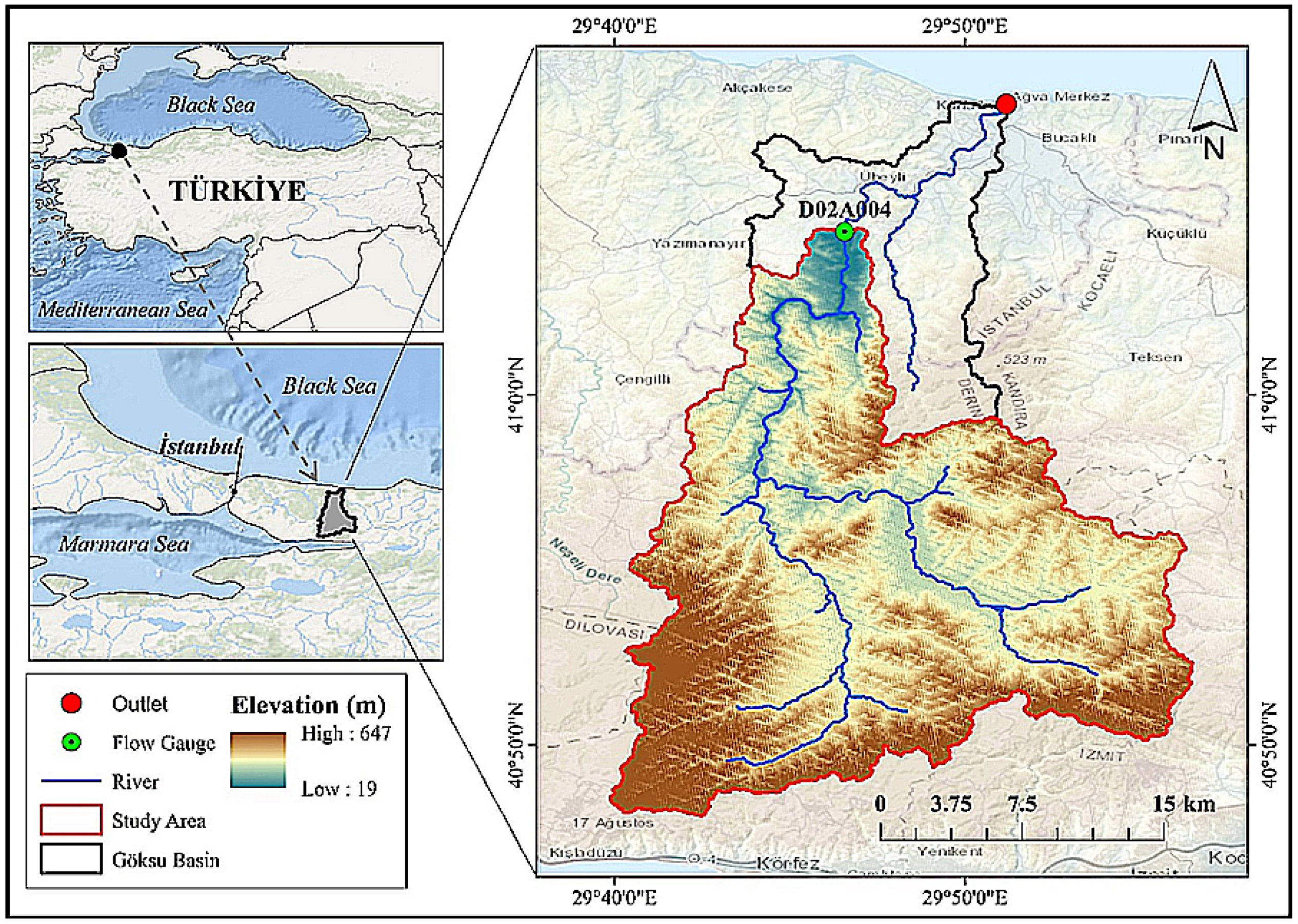
Göksu Stream is a stream originating from the Marmara Region of Türkiye and flowing into the Black Sea. Göksu Basin is located within the borders of Istanbul and Kocaeli provinces in Türkiye. The total basin area is approximately 482 km². Göksu Stream flows into the Black Sea from the Ağva neighborhood of Istanbul Province. Ağva is an important touristic coastal town located on the Black Sea coast of Istanbul. That is why the population increases threefold in summer [39]. The region is confronted with a critical scarcity of water resources, a situation exacerbated by the concentration of tourist accommodations, beaches, and a marked population surge during the summer months. There are two artificial lakes and one regulator on Göksu Stream. In addition, strategic planning is in progress for the construction of a dam, an initiative aimed at securing a sustainable water supply for Istanbul in the foreseeable future. This proactive measure underscores a comprehensive approach to addressing the water scarcity challenge, highlighting the innovative strategies adopted to ensure the adequacy of water resources in response to both current needs and future demands. In the scope of this research, the study area was defined to encompass the Göksu Basin outlet, which is represented by flow station named D02A004 within the basin’s stream network. Figure 1 describes the region determined as the study area. Accordingly, the drainage area at the flow station (D02A004) is about 395 km² [40]. Approximate mean elevation is 295 m, varying from 19 m to 647 m. The mainstream length is 43 km with many tributaries feeding the river. The flow data for station D02A004 were obtained from the head office of the General Directorate of State Hydraulic Works (DSİ) in Istanbul, Turkey. Monthly streamflow data covers the period 1984–2022.

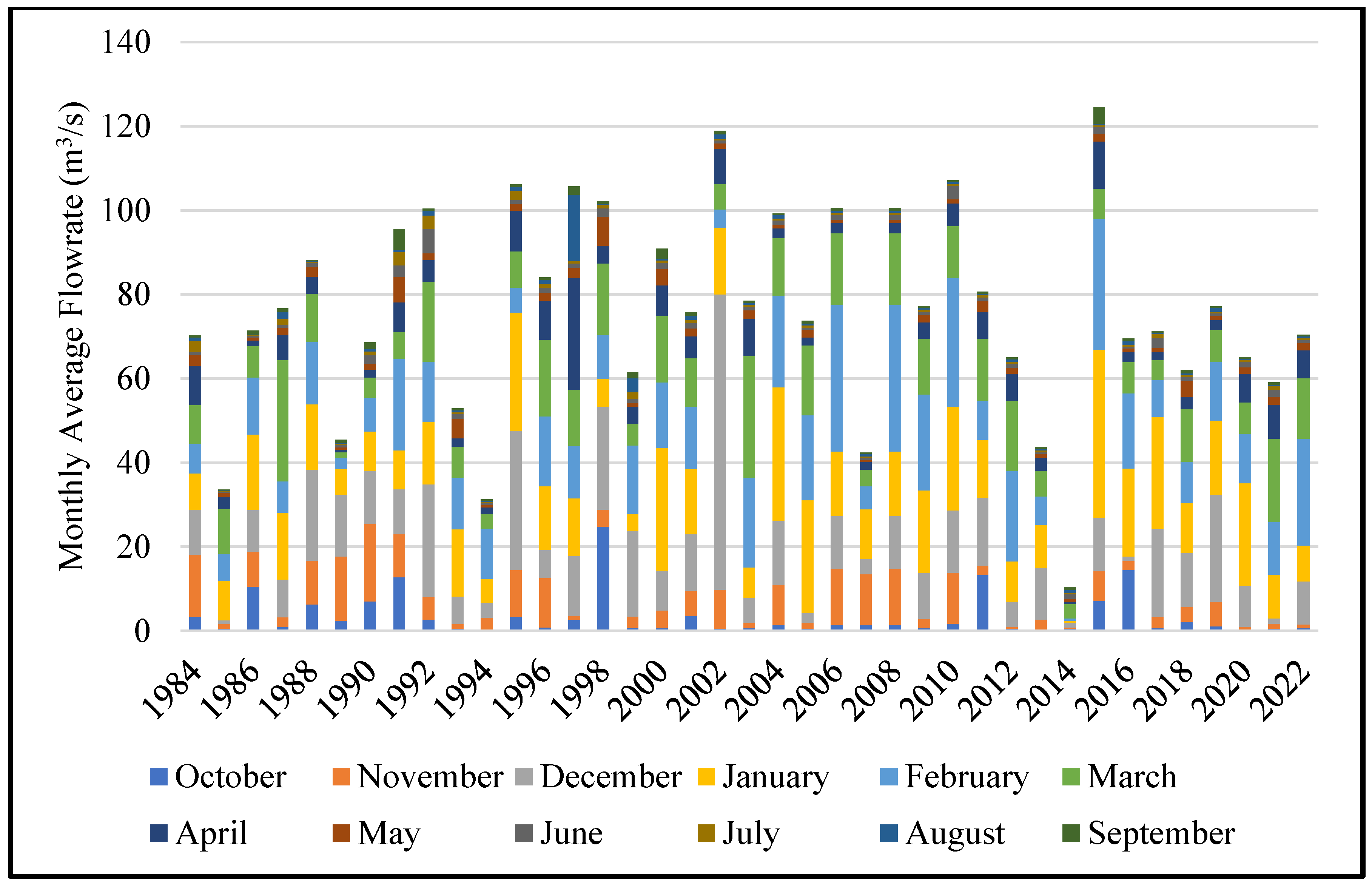
Figure 2 shows that monthly average flowrates of Göksu Stream between 1984 and 2022. Considering the highest and lowest averages, although 2014 was quite dry in terms of precipitation, the flow rate reached its highest level in the following year with the effect of precipitation. Although the Göksu Basin varies each year that receives the highest rainfall in the December-February period and the lowest rainfall in the June-August period. The amount of precipitation in the winter months is more intense than in the spring. Natural events and precipitation may not be consistent over the same period each year. As a result, various environmental challenges arise. Due to occasional flooding, especially the surrounding agricultural lands and biological ecosystems can be damaged. For these reasons, it is quite important to prevent flooding, mitigate its impacts and implement flood management strategies.

2.2. Machine Learning Methods

The machine learning models used in this study were selected based on their ability to handle the complexity of nonlinear dataset in hydrological systems affected by various environmental factors. Several different machine learning models were tested in the feasibility studies prior to the study. Considering the data structure, XGBoost, RF and SVM algorithms were selected in this study.

2.2.1. Extreme Gradient Boosting (XGBoost)

ANN finds use in various fields, especially classification, modeling and prediction processes. The XGBoost method, one of the improved algorithms of the artificial neural networks set, is an innovative machine learning algorithm whose article was first published by Chen and Guestrin (2016) [41]. The published article was met with interest by data scientists. The XGBoost algorithm is an optimized variant of the Gradient Boosting algorithm. The advantages it provides over previous versions are the most important reason for the widespread use of XGBoost. XGBoost uses the maximum depth value when building the tree. If the created tree shows excessive downward progress, pruning is performed. In this way, overlearning is prevented. While the Gradient Boosting algorithm uses a first-order function to calculate the loss function, XGBoost performs these calculations using second-order functions [41].

XGBoost operates within the boosting framework, an ensemble technique that combines weak learners sequentially to form a strong learner, typically using decision trees [42]. The core of the algorithm is the optimization of a regularized objective function that balances the model’s fidelity to the data against its complexity (Equation (1)) [41].

$$L(\mathit{\theta }) = {\sum }_{i=1}^n{l(Y}_i-{\mathit{ý}}_i)+{\sum }_{k=1}^K\mathit{\Omega } (f_k)$$

(1)

where, L (θ) is the total loss to be minimized, l represents a differentiable convex loss function measuring the discrepancy between the prediction ý_i and the actual target Y_i, f_k denotes the regularization term, defined as Ω, f_k = ƔT + ½ λ ||W||², with T representing the tree’s number of leaves, W is the scores on leaves, Ɣ is the complexity.

2.2.2. Random Forest (RF)

RF, proposed as a combination of decision trees, is used as an improved version of the bagging method by adding the randomness feature [43]. RF algorithm is an algorithm that helps solve regression problems within the decision tree. It also enables creating a subtree with randomly selected features within the created tree. There is no pruning process for the trees within the algorithm. The random tree algorithm can have a high accuracy rate in evaluations with the large number of random trees created [43,44]. One of the most important advantages of the algorithm is that it solves the overfitting problem in decision trees. The random tree method uses tree type classifier as follows (Equation (2)):

$$\begin{gathered} \{\mathcal{ℎ}(x, {\mathit{\theta }}_k)k=1, \dots \} \\ \sum \sum _{j \ne i}\left(f\right(Ci , T)/|T\left|\right)\left(f\right(Cj , T)/|T\left|\right) \end{gathered}$$

(2)

The input data is x and the random vector is represented by θ_k [44]. The random tree algorithm uses the GINI index given below to determine the best branch among the available branches [45]. T is the training data set, C_i is the class to which the data belongs, f (C_i, T)/|T|. It shows the probability that the selected data belongs to the C_i class [46,47]. The random tree algorithm provides better generalization and accurate prediction than other algorithms because it includes random sampling and an improved structure of ensemble algorithms techniques [47].

2.2.3. Support Vector Machine (SVM)

SVM is a machine learning algorithm based on statistical learning theory. This algorithm, which can classify and predict both linear and non-linear data, is frequently used in regression and classification problems. This method creates an optimal separating hyperplane that divides the data into two separate categories using support vectors and class intervals. The main purpose that is optimally separate the data points with a hyperplane. Then, the original training data is transformed using a non-linear mapping in a higher dimension. This transformation ensures that a hyperplane can always be used to separate data into two different classes [48,49]. Mathematically, the SVM decision function for binary classification can be expressed as follows:

$$f\left(x\right)=sign+\sum _{i=0}^{N}yi \mathit{\alpha }i K \left(x, xi\right)+ b$$

(3)

where, f(x) is the prediction of the example class, x is the example to be predicted, yi is the label of the i-th support vector, αi is the Lagrange multiplier of the i-th support vector, K (x,xi) is the Kernel function (a transformed version of the dot product between x and xi), b is the bias term of the decision function.

The kernel function used here allows SVM to operate in higher dimensional spaces with a technique called kernel trick.

2.3. Statistical Methods

The statistical methods used in this study are methods that aim to estimate the flowrate in a certain time period by using seasonality and time series for the analysis of flow data. These methods have been successfully applied in similar studies in the literature. Although there are many different statistical methods in the literature, it is possible to analyze seasonal and sudden changes in stream with time series. SES and ARIMA methods are preferred in this study thanks to the suitability of the available data structure.

2.3.1. Simple Exponential Smoothing (SES)

SES is a statistical method used to predict future values of a time series. This method aims to predict future values by making heavy use of historical data. SES method includes three basic components that form time series smoothing, smoothed forecasts and future forecasts. These are level, trend and seasonality. SES predicts future values using a combination of these three components. Essentially, the impact of historical data diminishes relative to the past. However, it allows important features such as level, trend and seasonality to be taken into account over time [50]. Here, the parameter values of SES are used as follows in the literature (Equation (4)) [51]:

$${\mathit{ý}}_t=\mathit{\alpha }· {\mathit{\gamma }}_{t-1} + (1-\mathit{\alpha })·{\mathit{ý}}_{t-1}$$

(4)

where, ý_t is the predicted value at time t, γ_t−1 is the actual value of the previous time, ý_t−1 is the predicted value of the previous time, α is the parameter used between values 0–1.

2.3.2. Autoregressive Integrated Moving Average Model (ARIMA)

ARIMA (p, d, q) Box Jenkins Model proposed by Box and Jenkins is one of the common methods used to create a univariate time series forecasting model [52]. An ARIMA process is a mathematical model used for prediction. Box-Jenkins modeling involves defining an appropriate ARIMA process, fitting it to the data, and then using the appropriate model for prediction. One of the attractive features of the Box Jenkins approach to forecasting is that ARIMA processes include a very rich class of models and generally provide adequate explanation of the data [53]. A non-seasonal ARIMA model is denoted by ARIMA (p, d, q), which is a combination of Autoregressive (AR) and Moving Average (MA) and the order of integration or divergence [54]. In general, the ARIMA model is as follows (Equation (5)):

Δd Zt = c + (Ø1 Δd Zt − 1 + … + Øp Δd Zt − p) − (θ1 et − 1 + … + θq et − q) + et
ΔZt = Zt − Zt − 1 Δ2 Zt − 1 = ΔZt − ΔZt − 1

(5)

where, c is the constant term, θq is the q-th moving average parameter, and et − k is the error term at time tk, Øp is the p-autoregressive parameter, and et is the error term at time t, Δ denotes the difference as shown below. Zt − 1 and Zt − p are the values of the past series with delays of 1 and p, respectively.

2.4. Model Performance Metrics

In this study, some performance criteria were used to show the goodness of fit of the models. These are the correlation coefficient (r), mean absolute error (MAE), root mean square error (RMSE), mean absolute percentage error (MAPE), coefficient of determination (R²), and Nash–Sutcliffe efficiency (NSE).

The correlation coefficient (r) quantifies the degree of closeness of points in a scatter plot to a linear regression line formed by those points (Equation (6)). It varies between −1 and +1. A value of −1 signifies a perfectly linear negative correlation (sloping downward), while a value of +1 signifies a perfectly linear positive correlation (sloping upward). The correlation coefficient, r, is directly related to the coefficient of determination R² in an obvious way (Equation (7)). The R² value is a measure of how well the regression line approximates the observed data, taking a value between 0 and 1. When R² = 1, it suggests a perfect fit. And, when R² = 0, it indicates no discernible relationship between the two variables.

$$r=\frac{n \left(\sum xy\right)-\left(\sum x\right)\left(\sum y\right)}{\sqrt{\left[n\sum x^2-{\left(\sum x\right)}^2\right]\left[n\sum y^2-{\left(\sum y\right)}^2\right]}}$$

(6)

where, n is the number of observations, ∑xy is the Sum of the products of x and y values, ∑x and ∑y are the sum of x and y values, ∑x² and ∑y² are the sum of the squares of x and y values.

$${\mathrm{R}}^2=1-\frac{\sum {\left({\mathrm{y}}_{\mathrm{i}}-{\mathbf{ý}}_{\mathrm{i}}\right)}^2}{\sum {\left({\mathrm{y}}_{\mathrm{i}}-\overline{\mathrm{y}}\right)}^2}$$

(7)

where, y_i is the actual y values, ý_i is the predicted y values (output of the regression equation), $\overline{y}$ is the mean of y values.

The MAE is the sum of the absolute value of the differences between the actual values and the predicted values in the data set divided by the number of samples (Equation (8)). The mean absolute error takes values between $0$ and $\infty$. The lower the value, the better the performance.

$$MAE=\frac{1}{n}=\sum _{i=1}^n\left|X_i-X\right|$$

(8)

The RMSE is the sum of the squares of the differences between the actual and predicted values in the data set, divided by the number of samples (Equation (9)). If there are outliers, the mean square error may be high. However, RMSE is calculated by taking the square root of the value found.

$$RMSE=\sqrt{\frac{1}{n}{\sum }_{i=1}^n{x}_t^2}$$

(9)

The MAPE is a statistical measure of the prediction accuracy of a prediction method (Equation (10)). It is also used as a loss function in machine learning problems. MAPE scales the size of the error as a percentage [55].

$$MAPE=\frac{1}{N}\sum _{t=1}^n\left|\frac{A_t-F_t}{A_t}\right|$$

(10)

where, $n$ is the number of fitted points, A_t is the actual value, F_t is the forecast value.

The model first proposed by Nash and Sutcliffe approached calibrations from a linear regression perspective. Particularly in hydrology, Nash–Sutcliffe efficiency (NSE) is one of the most important measurements used to perform model comparison and validation [56] (Equation (11)).

$$NSE=1-\frac{\sum _i{(O_i-S_i)}^2}{\sum _i{(O_i-{\overline{O}}_i)}^2}$$

(11)

where, S_i and O_i denote simulations and observations,${\overline{O}}_i$ is the observed mean.

3. Results

Forecasting of flowrates was conducted employing machine learning methods XGBoost, RF and SVM, and statistically ARIMA and SES methods, using streamflow data obtained from the Göksu Stream between 1984 and 2022. The dataset of this study was divided into 70% training and 30% testing. Then, the amount of data was divided equally by cross-validation method. Separate success percentages were calculated to determine the performance of each model used separately. The data used in this study was first trained with artificial neural networks and validated with 1984–2020 data. The dataset covering the years 1984 to 2020 was utilized as the training set, while the data from 2021 to 2022 served as the test set for evaluation purposes.

3.1. Machine Learning Methods Results

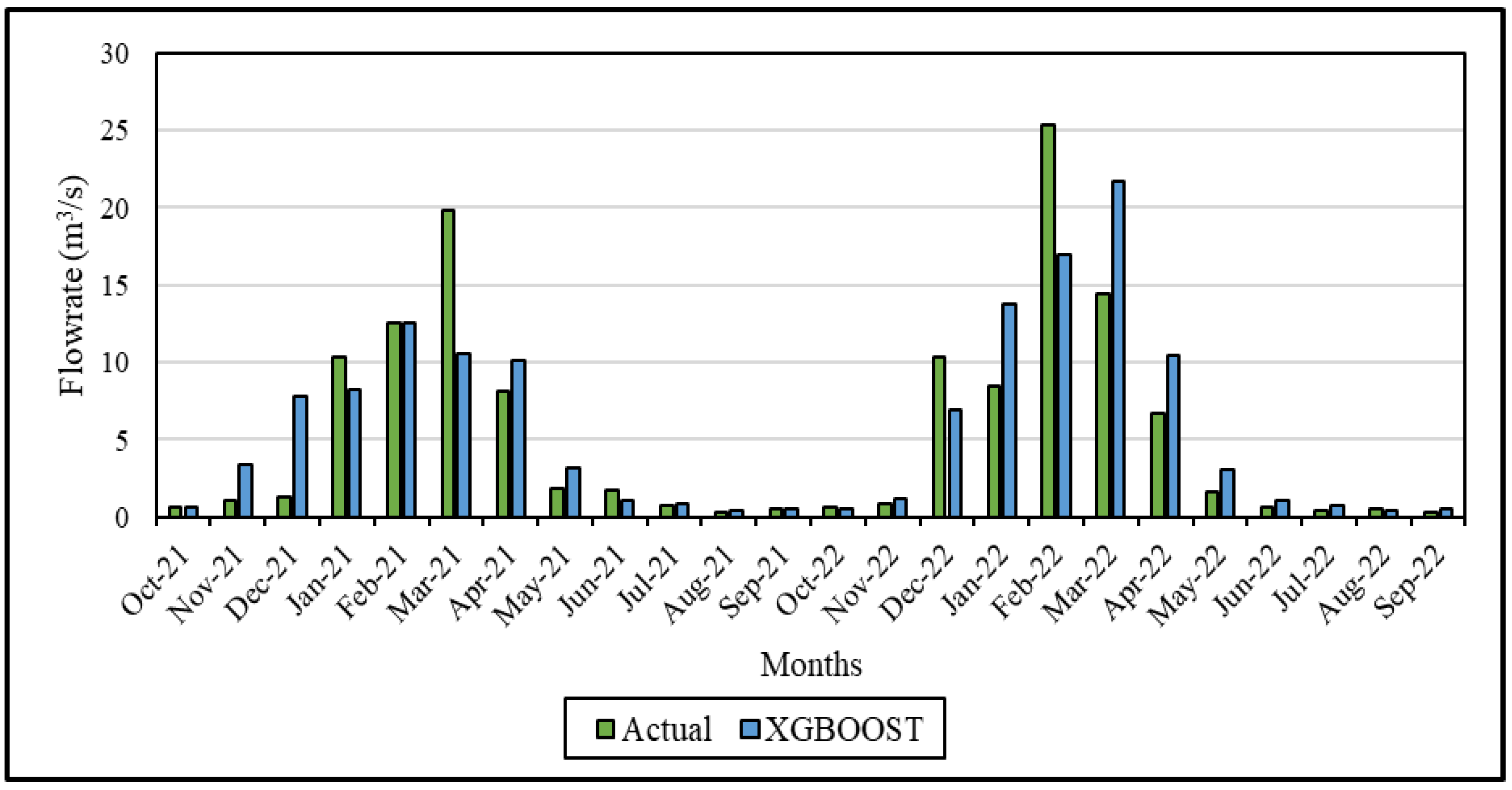
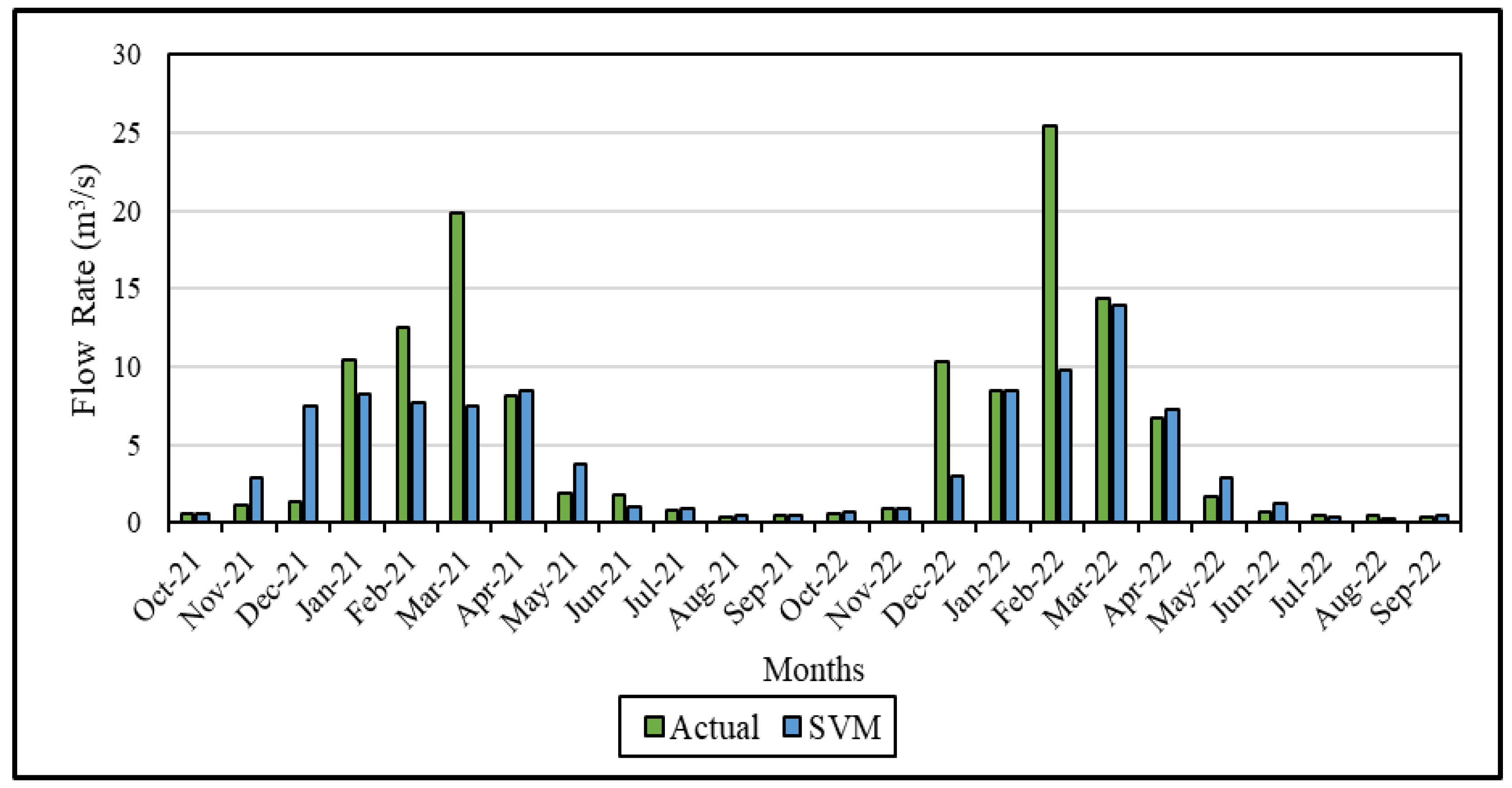
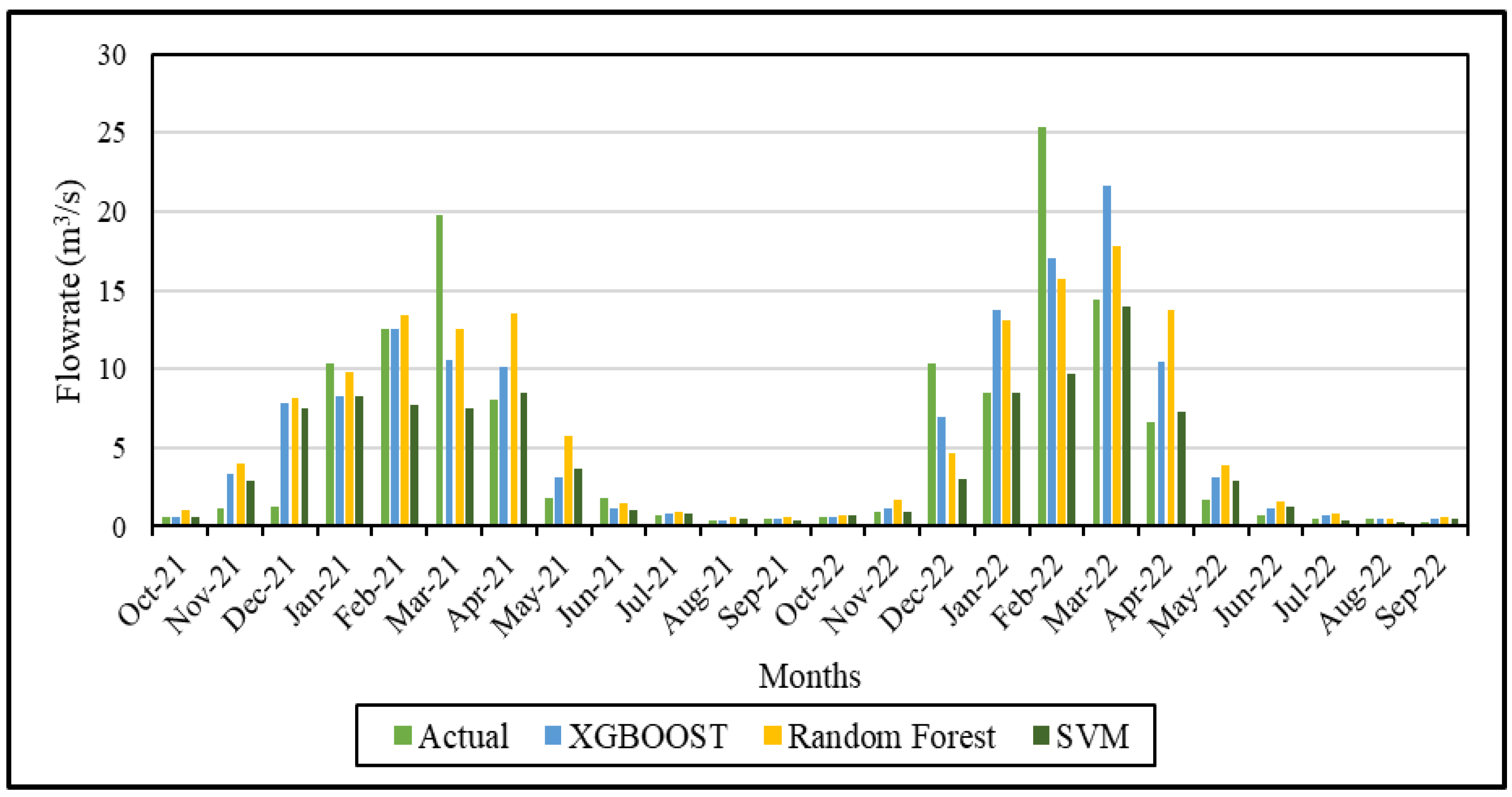
Figure 3, Figure 4 and Figure 5 depict the comparative analysis between actual and predicted data for XGBoost, RF and SVM modeling, respectively. Figure 6 illustrates a comparative graphic presenting all ANN model simulation results alongside the actual data.

In Figure 3, a notable observation is the highest percentage of error occurring between the actual and predicted values in February and March of 2022. In addition, since the expected precipitation in April is lower than in previous years, there is a difference between the predicted value and the actual value. Similarly, in 2021, the highest difference is again observed in March. The reason for this is that two years in a row, floods occurred in this region as a result of excessive rainfall. The sudden increase in water volume led to anomalies in the observations, a situation evident in the dataset. The difference between the actual and predicted values in November and December in the same year is due to the fact that the region receives rainfall below seasonal norms. The prediction model employed is unable to anticipate such abrupt fluctuations. However, a good agreement was observed between the actual and predicted values in January and February 2021. The margin of error appears to be negligible in this context. While there were substantial differences, particularly in December and March, close estimates were achieved with errors below 5% from June to November. It is noticeable that the calculated error is significantly lower, especially during the summer months or when rainfall amounts are diminished. Therefore, both the data set and the mathematical structure of the XGBoost algorithm directly affect the results.

Figure 4 shows that the RF model shows quite consistent results during the summer months within every two years. However, there is a difference between actual and predicted values due to sudden natural events in November–December and April–May 2021, April 2022. Unusual weather patterns not captured well by the model’s training data lead to inaccuracies in predictions. In summer seasons, the margin of error is calculated below 5%. According to the XGBoost model, it is seen that the predictions made in the summer months when precipitation is low and the data are consistent are closer to the reality.

Figure 5, shows that forecasts are far from the actual values in November-December-March 2021 and February 2022, when natural phenomena change rapidly. Like other machine learning algorithms, it is evident that the results obtained in periods with low precipitation are close to reality. Especially in the months with high flow rates, the predicted error rates increase. March-2021 and February-2022 are the months with the highest difference between actual and predicted values. Compared to the XGBoost algorithm, in these two machine learning algorithms, as the amount of streamflow increases, the difference between the actual and predicted values begins to increase. This allows us to observe the performance of each dataset across various models.

In Figure 6, the results of three machine learning models are provided alongside the actual values. For a more precise assessment of the model’s performance, it is advisable to utilize metrics such as the R² value or other performance indicators based on these test data. The R² values calculated for XGBoost, RF, and SVM are 0.72, 0.68, and 0.61, respectively. A R² value of 0.72 for XGBoost indicates that the model explains a substantial portion of the variance in the dependent variable. This implies that the model consistently responds to changes in the independent variables associated with the dependent variable, thereby showcasing its effectiveness as a predictive tool in real-world scenarios. R² value exceeding 60% signifies that the model effectively explains the independent variables associated with the dependent variable. When the R² value is above 60%, it generally implies that the model makes forecasts better than the mean value and that the flow rate forecasts are reliable.

The highest values for the correlation coefficients of the estimated data are 0.845, 0.825, and 0.778 for XGBOOST, RF, and SVM, respectively. The correlation coefficient seriously affects the accuracy of the forecasts. Therefore, the correlation scale is always taken into consideration in experimental studies that require measurement. Hence, the closer the forecasts of the model are to the actual data, the more reliable the model is for these data.

The highest MAPE percentage RF value found for the predicted 2021 and 2022 values is 87.08%. MAPE is used to determine the degree to which a model or forecast is correct or incorrect. It is used as an indicator of how accurately a model can predict future forecasts. It is therefore often used as a measure of accuracy. The results of other evaluation criteria are given in Table 1.

The performance metrics, as shown in Table 1, unequivocally demonstrate how well the XGBoost model outperforms rival forecasting models on a number of important fronts. The robust association between the predicted and actual values is demonstrated by the XGBoost model, which has a correlation coefficient of 0.845. It’s remarkable accuracy in forecasting values is demonstrated by its lowest MAE of 2.294 and lowest RMSE of 3.664. With a MAPE of 62.28%, the XGBOOST model likewise obtains the lowest, demonstrating its capacity to produce forecasts with little percentage difference from the actual data. Moreover, XGBoost has the maximum score of 0.711 for the NSE, which measures predictive capability.

3.2. Statistical Methods Result

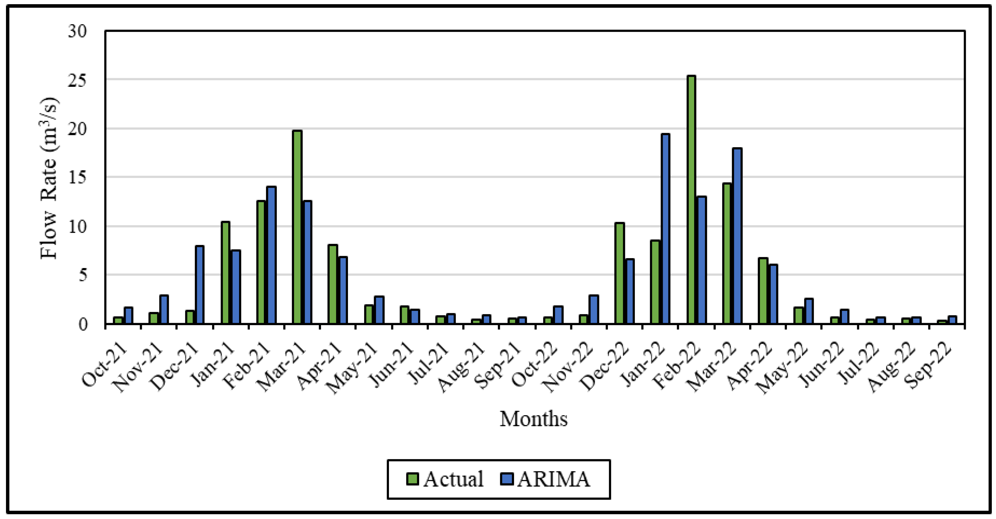
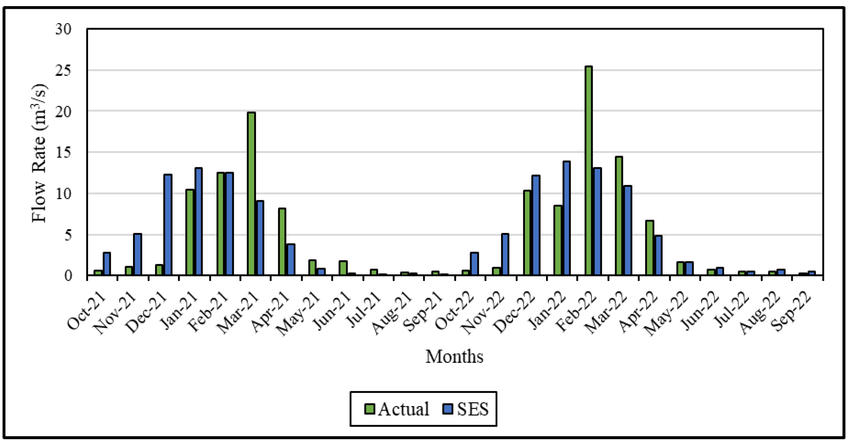
Figure 7 and Figure 8 show the data for the actual and predicted values for 2021–2022 generated by statistical methods. When Figure 7 is analyzed, it is evident that the largest disparity between the actual and predicted values occurs in March 2021 and February 2022. In November-December 2021 and January–February 2022, there is an inconsistency in the predicted values as a result of the anomaly caused by natural phenomena. The fact that the highest percentage of error is observed in the winter months in both years seems to be related to precipitation and thus the increase in the amount of data. Also, Figure 8 shows that the predicted and actual error percentages are quite low, especially in the summer months. Considering the performance metrics in Table 1, the SES model achieves the highest MAPE value. It shows that statistical methods used in time series analysis cannot make successful predictions in the case of sudden changes.

When analyzing Figure 7, similar to Figure 8, it can be observed that the error rates between actual and predicted values during the winter months across the two years. In the predictions made in October-December and March-April 2021, the predictions were made with much larger numbers compared to the ARIMA method. The highest error percentages are found in the SES method. The most significant disparity emerges in February 2022, where despite the actual flow rate being 25 m³/s, the model predicted a considerably lower value. This discrepancy resulted in an error percentage of 44%, marking the highest error rate in this study.

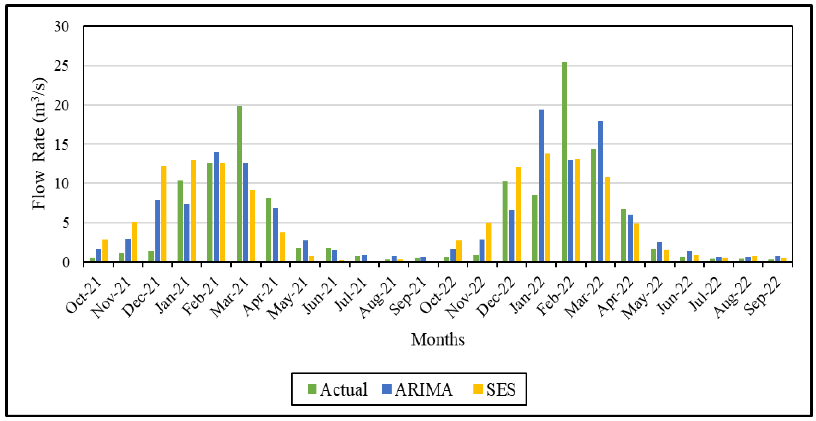
In Figure 9, the results of two statistical models are presented alongside the actual values. The R2 values calculated for ARIMA and SES are 0.63 and 0.55, respectively. The R² value of 0.55 suggests that the model insufficiently explains the relationship between independent variables and the dependent variable in the case of SES. However, it is seen that statistical forecasts except for the summer months have high error percentages and lower forecast performances compared to machine learning methods.

Figure 9. The comparison between actual and predicted data for ARIMA and SES in the modeling period (2021–2022).

Figure 9. The comparison between actual and predicted data for ARIMA and SES in the modeling period (2021–2022).

Table 1. Performance metrics for the simulations of machine learning and statistical methods.

	Machine Learning Methods			Statistical Methods
Performance Metrics	XGBOOST	RF	SVM	SES	ARIMA
R2	0.72	0.68	0.61	0.55	0.63
r	0.845	0.825	0.778	0.74	0.79
MAE	2.294	2.659	2.36	2.94	2.55
RMSE	3.664	3.919	4.683	4.59	4.19
MAPE	62.28%	87.08%	68.40%	133.40%	92.70%
NSE	0.711	0.669	0.528	0.546	0.622
Total Number of Instances	24	24	24	24	24

Table 1. Performance metrics for the simulations of machine learning and statistical methods.

	Machine Learning Methods			Statistical Methods
Performance Metrics	XGBOOST	RF	SVM	SES	ARIMA
R2	0.72	0.68	0.61	0.55	0.63
r	0.845	0.825	0.778	0.74	0.79
MAE	2.294	2.659	2.36	2.94	2.55
RMSE	3.664	3.919	4.683	4.59	4.19
MAPE	62.28%	87.08%	68.40%	133.40%	92.70%
NSE	0.711	0.669	0.528	0.546	0.622
Total Number of Instances	24	24	24	24	24

4. Discussion

The predictive performance of three different machine learning techniques and two statistical methods employed in this study was evaluated using various success metrics. The irregular behavior of some natural phenomena involved in hydrological studies requires some pre-processing to ensure these conditions before modeling. However, in modeling using artificial intelligence models, all natural phenomena can be modeled in a simple way without any pre-processing. In the evaluation made for the correlation coefficient depending on the amount of data in all models, it was observed that all models produced prediction data that converged to the targeted data in high correlation. As the general evaluation criterion, the correlation coefficients of the three different machine learning models were found to be at least 0.78. This shows the confidence rate of the model and the correct relationship between the data. Additionally, XGBoost model has the lowest error rate with MAE and RMSE ratios of 2.294 and 3.664, respectively. Examining the actual values from 2021 to 2022 alongside the forecasts generated by machine learning methods reveals that particularly during the summer months, the forecasts closely align with the actual values, resulting in very low error rates. When we look at the figure of three models, it is seen that all actual and predicted values are consistent except for March 2021 and February 2022. The reason for the inconsistencies for these two months is the flooding and inundation explained separately in the result section. As shown in Table 1, the consistency rate of the forecasts is high. According to the MAPE results, the XGBoost algorithm performed better than RF and SVM. One of the main reasons for this is that the algorithm is suitable for complex hydrological modeling tasks due to its ability to analyze non-linear relationships and high-dimensional data. Furthermore, the NSE, a commonly utilized metric in studies of hydrology and water resources management, is employed to assess the accuracy of model predictions. XGBoost model achieved the highest NSE accuracy rate of 0.711. Considering the results of machine learning models, XGBoost model suitable forecast models for hydrological studies.

Considering the outcomes derived from the two different statistical methods employed in the study, the performance metrics have reached lower success percentages compared to machine learning methods. Although the correlation coefficients of both methods are at acceptable levels of 0.74 and 0.79 for ARIMA and SES, respectively, MAPE values are well above the acceptance limits. Especially the MAPE value of the SES model is around 133% and the predicted values are significantly different from the actual values. Therefore, this is not acceptable as the percentage error between actual and predicted values is much higher than expected. The reason why the margin of error in statistical analysis using time series is considerably higher than in machine learning methods is that sudden changes (floods, storms, etc.) cannot be calculated statistically. As a result, all statistical data is based on historical data and attempts to draw meaningful inferences from it. In artificial intelligence algorithms, on the other hand, it is understandable that the data is divided into a test and training set, first trained and then tested with real data, resulting in realistic values and high accuracy percentages. Then, all the findings of our study are analyzed and brought together and the data set is taken into consideration, the analysis obviously indicates that the XGBoost model is the best choice for generating accurate forecasts.

5. Conclusions

In this study, it was aimed to forecast the monthly average streamflows measured on Göksu Stream with machine learning and statistical methods. The average monthly streamflow data obtained from DSI for the years 1984–2022 were processed and estimated by machine learning (XGBoost, RF and SVM) and statistical (SES and ARIMA) methods. The accuracy of the models was demonstrated by statistical comparison of actual (observed) and predicted values. Moreover, models were compared in terms of monthly streamflow forecast. Finally, various performance metrics such as correlation coefficient (r), mean absolute error (MAE), root mean square error (RMSE), mean absolute percentage error (MAPE), coefficient of determination (R²) and Nash–Sutcliffe efficiency (NSE) were calculated to assess model accuracy and examine error percentages. Therefore, the following conclusions have been reached based on the outcomes of this study:

• The study confirmed the effectiveness of selected machine learning and statistical methods in predicting streamflows, demonstrating their utility in hydrological studies.
• The findings indicated the potential of these methods to support decisions related to water resource systems.
• For a variety of hydrological and environmental applications, including flood flowrate estimation, hydroelectric generation, and water resource management, the study highlights the need of precise streamflow forecast.
• The prediction results calculated in the study coincide with the actual streamflow data. After analyzing all the findings from our study and considering the dataset, it is concluded that the XGBoost model is the best choice for making accurate forecasts.
• The study successfully demonstrates the effectiveness of machine learning and statistical methods in forecasting monthly average streamflows, highlighting their crucial role in hydrological studies and related applications.
• It underscores the importance of continuous innovation in modeling techniques and dataset diversification for improving flood predictions, essential for effective basin management and urban planning. Overall, the study contributes to advancing the field of hydrology and provides valuable insights for future research and application.

References

- Erdal, H.I.; Karakurt, O. Advancing monthly streamflow prediction accuracy of CART models using ensemble learning paradigms. J. Hydrol. 2013, 477, 119–128. [Google Scholar] [CrossRef]
- Ni, L.; Wang, D.; Singh, V.P.; Wu, J.; Wang, Y.; Tao, Y.; Zhang, J. Streamflow and rainfall forecasting by two long short-term memory-based models. J. Hydrol. 2020, 583, 124296. [Google Scholar] [CrossRef]
- Yaseen, Z.M.; El-Shafie, A.; Jaafar, O.; Afan, H.A.; Sayl, K.N. Artificial intelligence-based models for stream-flow forecasting: 2000–2015. J. Hydrol. 2015, 530, 829–844. [Google Scholar] [CrossRef]
- Fathian, F.; Mehdizadeh, S.; Sales, A.K.; Safari, M.J.S. Hybrid models to improve the monthly river flow prediction: Integrating artificial intelligence and non-linear time series models. J. Hydrol. 2019, 575, 1200–1213. [Google Scholar] [CrossRef]
- Tongal, H.; Booij, M.J. Simulation and forecasting of streamflows using machine learning models coupled with base flow separation. J. Hydrol. 2018, 564, 266–282. [Google Scholar] [CrossRef]
- Shafizadeh-Moghadam, H.; Valavi, R.; Shahabi, H.; Chapi, K.; Shirzadi, A. Novel forecasting approaches using combination of machine learning and statistical models for flood susceptibility mapping. J. Environ. Manag. 2018, 217, 1–11. [Google Scholar] [CrossRef]
- Dalkılıç, H.Y.; Yeşilyurt, S.N.; Samui, P. Daily flow modeling with random forest and k-nearest neighbor methods. Erzincan Univ. J. Sci. Technol. 2021, 14, 914–925. [Google Scholar]
- Nazimi, N.; Saplıoğlu, K. Monthly streamflow prediction using ANN, KNN and ANFIS models: Example of Gediz River Basin. Tek. Bilim. Derg. 2023, 13, 42–49. [Google Scholar] [CrossRef]
- Stakhiv, E.; Stewart, B. Needs for climate information in support of decision-making in the water sector. Procedia Environ. Sci. 2010, 1, 102–119. [Google Scholar] [CrossRef]
- Nourani, V.; Komasi, M. A geomorphology-based ANFIS model for multi-station modeling of rainfall–runoff process. J. Hydrol. 2013, 490, 41–55. [Google Scholar] [CrossRef]
- Xiao, Z.; Liang, Z.; Li, B.; Hou, B.; Hu, Y.; Wang, J. New flood early warning and forecasting method based on similarity theory. J. Hydrol. Eng. 2019, 24, 04019023. [Google Scholar] [CrossRef]
- Latifoğlu, L. A novel approach for prediction of daily streamflow discharge data using correlation-based feature selection and random forest method. Int. Adv. Res. Eng. J. 2022, 6, 1–7. [Google Scholar] [CrossRef]
- Kisi, O.; Latifoğlu, L.; Latifoğlu, F. Investigation of empirical mode decomposition in forecasting of hydrological time series. Water Resour. Manag. 2014, 28, 4045–4057. [Google Scholar] [CrossRef]
- Petty, T.R.; Dhingra, P. Streamflow hydrology estimate using machine learning (SHEM). J. Am. Water Resour. Assoc. 2018, 54, 55–68. [Google Scholar] [CrossRef]
- Lin, Y.; Wang, D.; Wang, G.; Qiu, J.; Long, K.; Du, Y.; Xie, H.; Wei, Z.; Shangguan, W.; Dai, Y. A hybrid deep learning algorithm and its application to streamflow prediction. J. Hydrol. 2021, 601, 126636. [Google Scholar] [CrossRef]
- Xiang, Z.; Demir, I. Distributed long-term hourly streamflow predictions using deep learning–A case study for State of Iowa. Environ. Model. Softw. 2020, 131, 104761. [Google Scholar] [CrossRef]
- Delaney, C.J.; Hartman, R.K.; Mendoza, J.; Dettinger, M.; Delle Monache, L.; Jasperse, J.; Martin Ralph, F.; Talbot, C.; Brown, J.; Reynolds, D.; et al. Forecast informed reservoir operations using ensemble streamflow predictions for a multipurpose reservoir in Northern California. Water Resour. Res. 2020, 56, e2019WR026604. [Google Scholar] [CrossRef]
- Malik, A.; Tikhamarine, Y.; Souag-Gamane, D.; Kisi, O.; Pham, Q.B. Support vector regression optimized by meta-heuristic algorithms for daily streamflow prediction. Stoch. Environ. Res. Risk Assess. 2020, 34, 1755–1773. [Google Scholar] [CrossRef]
- Asadi, H.; Shahedi, K.; Jarihani, B.; Sidle, R.C. Rainfall-runoff modelling using hydrological connectivity index and artificial neural network approach. Water 2019, 11, 212. [Google Scholar] [CrossRef]
- Snieder, E.; Shakir, R.; Khan, U.T. A comprehensive comparison of four input variable selection methods for artificial neural network flow forecasting models. J. Hydrol. 2020, 583, 124299. [Google Scholar] [CrossRef]
- Ikram, R.M.A.; Ewees, A.A.; Parmar, K.S.; Yaseen, Z.M.; Shahid, S.; Kisi, O. The viability of extended marine predators’ algorithm-based artificial neural networks for streamflow prediction. Appl. Soft Comput. 2022, 131, 109739. [Google Scholar] [CrossRef]
- Niu, W.J.; Feng, Z.K.; Chen, Y.B.; Zhang, H.R.; Cheng, C.T. Annual streamflow time series prediction using extreme learning machine based on gravitational search algorithm and variational mode decomposition. J. Hydrol. Eng. 2020, 25, 04020008. [Google Scholar] [CrossRef]
- Hussain, D.; Hussain, T.; Khan, A.A.; Naqvi, S.A.A.; Jamil, A. A deep learning approach for hydrological time-series prediction: A case study of Gilgit river basin. Earth Sci. Inform. 2020, 13, 915–927. [Google Scholar] [CrossRef]
- Adnan, R.M.; Yuan, X.; Kisi, O.; Yuan, Y. Streamflow forecasting using artificial neural network and support vector machine models. Am. Sci. Res. J. Eng. Technol. Sci. 2017, 29, 286–294. [Google Scholar]
- Le, X.H.; Nguyen, D.H.; Jung, S.; Yeon, M.; Lee, G. Comparison of deep learning techniques for river streamflow forecasting. IEEE Access 2021, 9, 71805–71820. [Google Scholar] [CrossRef]
- Saraiva, S.V.; de Oliveira Carvalho, F.; Santos, C.A.G.; Barreto, L.C.; Freire, P.K.D.M.M. Daily streamflow forecasting in Sobradinho Reservoir using machine learning models coupled with wavelet transform and bootstrapping. Appl. Soft Comput. 2021, 102, 107081. [Google Scholar] [CrossRef]
- Kagoda, P.A.; Ndiritu, J.; Ntuli, C.; Mwaka, B. Application of radial basis function neural networks to short-term streamflow forecasting. Phys. Chem. Earth 2010, 35, 571–581. [Google Scholar] [CrossRef]
- Yonaba, H.; Anctil, F.; Fortin, V. Comparing sigmoid transfer functions for neural network multistep ahead streamflow forecasting. J. Hydrol. Eng. 2010, 15, 275–283. [Google Scholar] [CrossRef]
- Zaini, N.; Malek, M.A.; Yusoff, M.; Mardi, N.H.; Norhisham, S. Daily River Flow Forecasting with Hybrid Support Vector Machine–Particle Swarm Optimization. IOP Conf. Ser. Earth Environ. Sci. 2018, 140, 012035. [Google Scholar] [CrossRef]
- Farias, C.A.; Santos, C.A.; Lourenço, A.M.; Carneiro, T.C. Kohonen neural networks for rainfall-runoff modeling: Case study of Piancó River Basin. J. Urban Environ. Eng. 2013, 7, 176–182. [Google Scholar] [CrossRef]
- Danandeh Mehr, A.; Kahya, E.; Şahin, A.; Nazemosadat, M.J. Successive-station monthly streamflow prediction using different artificial neural network algorithms. Int. J. Environ. Sci. Technol. 2015, 12, 2191–2200. [Google Scholar] [CrossRef]
- Adhikary, S.K.; Muttil, N.; Yilmaz, A.G. Improving streamflow forecast using optimal rain gauge network-based input to artificial neural network models. Hydrol. Res. 2018, 49, 1559–1577. [Google Scholar] [CrossRef]
- Prasad, R.; Deo, R.C.; Li, Y.; Maraseni, T. Input selection and performance optimization of ANN-based streamflow forecasts in the drought-prone Murray Darling Basin region using IIS and MODWT algorithm. Atmos. Res. 2017, 197, 42–63. [Google Scholar] [CrossRef]
- Alvisi, S.; Franchini, M. Fuzzy neural networks for water level and discharge forecasting with uncertainty. Environ. Model. Softw. 2011, 26, 523–537. [Google Scholar] [CrossRef]
- Aslan, M.F.; Sabanci, K.; Durdu, A. Different wheat species classifier application of ANN and ELM. J. Multidiscip. Eng. Sci. Technol. 2017, 4, 8194–8198. [Google Scholar]
- Dickey, D.A.; Fuller, W.A. Likelihood ratio statistics for autoregressive time series with a unit root. Econom. J. Econom. Soc. 1981, 49, 1057–1072. [Google Scholar] [CrossRef]
- Kazemi, M. A comparative study of singular spectrum analysis, neural network, ARIMA and exponential smoothing for monthly rainfall forecasting. J. Math. Model. 2023, 11, 783–803. [Google Scholar]
- Murat, M.; Malinowska, I.; Hoffmann, H.; Baranowski, P. Statistical modelling of agrometeorological time series by exponential smoothing. Int. Agrophys. 2016, 30, 57–65. [Google Scholar] [CrossRef]
- Fırat, A. Estimation of Average Flow and Maximum Precipitation by Artificial Neural Networks Case of Istanbul Göksu Stream. Master’s Thesis, Sakarya University, Serdivan, Türkiye, 2019. [Google Scholar]
- SYGM (General Directorate of Water Management, in Turkish: Su Yönetimi Genel Müdürlüğü). Marmara Basin Flood Management Plan; Republic of Türkiye Ministry of Agriculture and Forestry—General Directorate of Water Management: Ankara, Türkiye, 2023; pp. 1–1540. [Google Scholar]
- Chen, T.; Guestrin, C. Xgboost: A Scalable Tree Boosting System. In Proceedings of the 22nd ACM SIGKDD International Conference on Knowledge Discovery and Data Mining, San Francisco, CA, USA, 13–17 August 2016. [Google Scholar]
- Freund, Y.; Schapire, R.E. A decision-theoretic generalization of on-line learning and an application to boosting. J. Comput. Syst. Sci. 1997, 55, 119–139. [Google Scholar] [CrossRef]
- Breiman, L. Random forests. Mach. Learn. 2001, 45, 5–32. [Google Scholar] [CrossRef]
- Ali, J.; Khan, R.; Ahmad, N.; Maqsood, I. Random forests and decision trees. Int. J. Comput. Sci. Issues 2012, 9, 272. [Google Scholar]
- Pal, M. Random forest classifier for remote sensing classification. Int. J. Remote Sens. 2005, 26, 217–222. [Google Scholar] [CrossRef]
- Gislason, P.O.; Benediktsson, J.A.; Sveinsson, J.R. Random forests for land cover classification. Pattern Recognit. Lett. 2006, 27, 294–300. [Google Scholar] [CrossRef]
- Qi, Y. Random forest for bioinformatics. In Ensemble Machine Learning: Methods and Applications; Springer: New York, NY, USA, 2012; pp. 307–323. [Google Scholar]
- Atallah, R.; Al-Mousa, A. Heart Disease Detection Using Machine Learning Majority Voting Ensemble Method. In Proceedings of the 2nd International Conference on New Trends in Computing Sciences (ICTCS), Amman, Jordan, 9–11 October 2019. [Google Scholar]
- Shevade, S.K.; Keerthi, S.S.; Bhattacharyya, C.; Murthy, K.R.K. Improvements to the SMO algorithm for SVM regression. IEEE Trans. Neural Netw. 2000, 11, 1188–1193. [Google Scholar] [CrossRef] [PubMed]
- Billah, B.; King, M.L.; Snyder, R.D.; Koehler, A.B. Exponential smoothing model selection for forecasting. Int. J. Forecast. 2006, 22, 239–247. [Google Scholar] [CrossRef]
- Corberán-Vallet, A.; Bermúdez, J.D.; Segura, J.V.; Vercher, E. A forecasting support system based on exponential smoothing. In Handbook on Decision Making: Vol 1: Techniques and Applications; Springer: Berlin/Heidelberg, Germany, 2010; pp. 181–204. [Google Scholar]
- Mensah, E.K. Box-Jenkins Modelling and Forecasting of Brent Crude Oil Price; Munich Personal RePEc Archive; University Library of Munich: Munich, Germany, 2015; pp. 1–10. [Google Scholar]
- Hyndman, R.J. Box-Jenkins Modelling. In Regional Symposium on Environment and Natural Resources; John Wiley & Sons: San Francisco, CA, USA, 2001; pp. 10–11. [Google Scholar]
- Box, G.E.; Jenkins, G.M.; Reinsel, G.C.; Ljung, G.M. Time Series Analysis: Forecasting and Control; John Wiley & Sons: Hoboken, NJ, USA, 2015. [Google Scholar]
- Lewis, C.D. Industrial and Business Forecasting Methods; Butterworths Publishing: London, UK, 1982; ISBN 978-0408005593. [Google Scholar]
- Nash, J.; Sutcliffe, J.V. River flow forecasting through conceptual models’ part I—A discussion of principles. J. Hydrol. 1970, 10, 282–290. [Google Scholar] [CrossRef]
Figure 1.
The location, elevation, stream network, and streamflow observation stations within the Göksu Basin.
Figure 2.
The monthly average flowrate between 1984–2022 obtained from General Directorate of State Hydraulic Works (DSI).
Figure 3.
Comparative flow rate graph between actual and predicted data for XGBoost in the modeling period (2021–2022).
Figure 4.
Comparative flow rate analysis between actual and predicted data for RF in the modeling period (2021–2022).
Figure 5.
Comparative flow rate graph between actual and predicted data for SVM in the modeling period (2021–2022).
Figure 6.
The comparison between actual and predicted data for XGBOOST, RF, SVM in the modeling period (2021–2022).
Figure 7.
Comparative flow rate graph between actual and predicted data for ARIMA in the modeling period (2021–2022).
Figure 8.
Comparative flow rate graph between actual and predicted data for SES in the modeling period (2021–2022).
Disclaimer/Publisher’s Note: The statements, opinions and data contained in all publications are solely those of the individual author(s) and contributor(s) and not of MDPI and/or the editor(s). MDPI and/or the editor(s) disclaim responsibility for any injury to people or property resulting from any ideas, methods, instructions or products referred to in the content. |
© 2024 by the authors. Licensee MDPI, Basel, Switzerland. This article is an open access article distributed under the terms and conditions of the Creative Commons Attribution (CC BY) license (https://creativecommons.org/licenses/by/4.0/).
Share and Cite
MDPI and ACS Style
Ciner, M.N.; Güler, M.; Namlı, E.; Samastı, M.; Ulu, M.; Peker, İ.B.; Gülbaz, S. The Forecast of Streamflow through Göksu Stream Using Machine Learning and Statistical Methods. Water 2024, 16, 1125. https://doi.org/10.3390/w16081125
AMA Style
Ciner MN, Güler M, Namlı E, Samastı M, Ulu M, Peker İB, Gülbaz S. The Forecast of Streamflow through Göksu Stream Using Machine Learning and Statistical Methods. Water. 2024; 16(8):1125. https://doi.org/10.3390/w16081125
Chicago/Turabian StyleCiner, Mirac Nur, Mustafa Güler, Ersin Namlı, Mesut Samastı, Mesut Ulu, İsmail Bilal Peker, and Sezar Gülbaz. 2024. "The Forecast of Streamflow through Göksu Stream Using Machine Learning and Statistical Methods" Water 16, no. 8: 1125. https://doi.org/10.3390/w16081125
Note that from the first issue of 2016, this journal uses article numbers instead of page numbers. See further details here.