Decoupling Agricultural Grey Water Footprint from Economic Growth in the Yellow River Basin

Abstract

Decoupling agricultural economic growth from agricultural water pollution is of great importance to regional sustainable development. It is necessary to further explore the decoupling state and key driving factors connecting agricultural water pollution and agricultural economic growth on the basis of accurate measurement of agricultural water pollution. Accordingly, taking the Yellow River Basin (YRB) as the research object, this study combined the water footprint theory, the Logarithmic Mean Divisia Index (LMDI) model and the Tapio decoupling model (TDM) to conduct an in-depth decoupling analysis of the connection between the agricultural grey water footprint (AGWF) and agricultural economic growth in the YRB. Specifically, this study first calculated the AGWF of the YRB during 2016–2021 and objectively evaluated the water resource utilization in this region based on the AGWF. Then, the LMDI model was used to explore the driving factors of the AGWF in the YRB. Finally, the decoupling states between the AGWF and its driving factors with agricultural GDP (AGDP) were studied using the TDM. The main results are as follows: (1) The overall AGWF in the YRB showed a decreasing trend and a slow increase, decreasing by 5.39% in 2021 compared to 2016. (2) The primary promoting factor and inhibiting factor of AGWF reduction are the efficiency effect and agricultural economic effect, respectively. (3) The decoupling states of the AGWF and AGDP presented strong decoupling (SD) and then weak decoupling (WD) in the YRB during the research period. The decoupling states between the agricultural grey water footprint intensity (AGWFI) and AGDP changed from expansive negative decoupling (END) to SD. The decoupling state of population and AGDP remained SD. This study will contribute to alleviating agricultural water pollution in the YRB and help policymakers in water-stressed countries to formulate agricultural water management policies.

1. Introduction

Rapid economic growth, dramatic population expansion, and climate change have led to an exponential increase in water demand [1,2,3]. Globally, 1.5 billion people face severe and increasing water scarcity problems [4]. It is projected that this number will increase to 3.9 billion by 2050 [5]. Agricultural water occupies the highest proportion (70%) of freshwater resource utilization [6]. The leading cause of water pollution is agricultural non-point source pollution, which generates 75% of nitrogen-related global warming potential and 38% of phosphorus-related global warming potential [7,8,9]. More than 50% of nitrogen and phosphorus flows into water bodies due to inefficient use of fertilizers and pesticides [10]. The ineffective management of agricultural water pollution will result in a massive waste of resources and environmental damage. However, current studies have given little consideration to controlling pollutants produced by agricultural production [6,11]. With only 8% of the world’s arable land and a quarter of the global average per capita water supply, China needs to feed about 20% of the world’s population, which is also a considerable challenge [12]. Meanwhile, China’s agriculture has not fully realized large-scale operation, with low production efficiency and slow progress in adopting agricultural technology [13]. In this context, China can only continue to overuse fertilizers and pesticides to provide more food, becoming the fastest-growing country in the world for agrochemicals [14]. At the same time, animal husbandry aggravates agricultural grey water in China [15].

To quantitatively analyze water pollution, scholars put forward the grey water footprint, defined as the amount of polluted water diluted and managed to standard water quality according to natural concentration and current environmental water quality standards [16]. Researchers have recognized the need to manage and evaluate water resources by measuring the grey water footprint [17,18]. Regarding the measurement of agricultural water pollution, scholars either set up macroscopic hydrological models to conduct overall measurement analysis of agricultural grey water [7,11] or select only a few indicators to analyze the changing trend of water pollution [10,19,20]. In most of the published studies, the grey water footprint has been ignored or only partially considered because of the complexity of its calculation and the difficulty of its estimation due to the lack of data [21]. Although some studies can grasp the changes in agricultural grey water footprint, few of them have made accurate measurements of agricultural grey water footprint. In terms of driving factors of the agricultural grey water footprint (AGWF), scholars generally use the formula in the Water Footprint Assessment Manual [16] to calculate the AGWF more accurately from the two aspects of planting and breeding [15,18,22]. Still, more in-depth analyses of the specific factors that significantly impact the AGWF are needed. Therefore, some researchers introduced the Logarithmic Mean Divisia Index (LMDI) model to conduct in-depth studies of agricultural GDP (AGDP) driving factors [23,24]. Using the LMDI model for factor decomposition can avoid the impact of residual and zero values on the results, and it is a universally adaptable research method [25]. The LMDI model has been widely used in water resources and the environment. Zhang et al. utilized the LMDI model to explore the factor of AGWF decomposition in the midstream of the Heihe River from 1991 to 2015 only from the perspective of the planting industry [26]. Through the LMDI model, it was discovered that agricultural economic effect became the most critical factor in enhancing the AGWF efficiency [27]. In addition, it was found that AGDP and the intensity of the AGWF exerted the most significant promoting and inhibiting effects upon AGWF change in China, respectively [6]. According to the Sustainable Development Goals (SDGs), decoupling resources and environmental pressures from economic growth is integral. Although the LMDI model can identify the driving factors affecting the change in water resources, it cannot quantitatively measure the decoupling state between economic growth and water consumption.

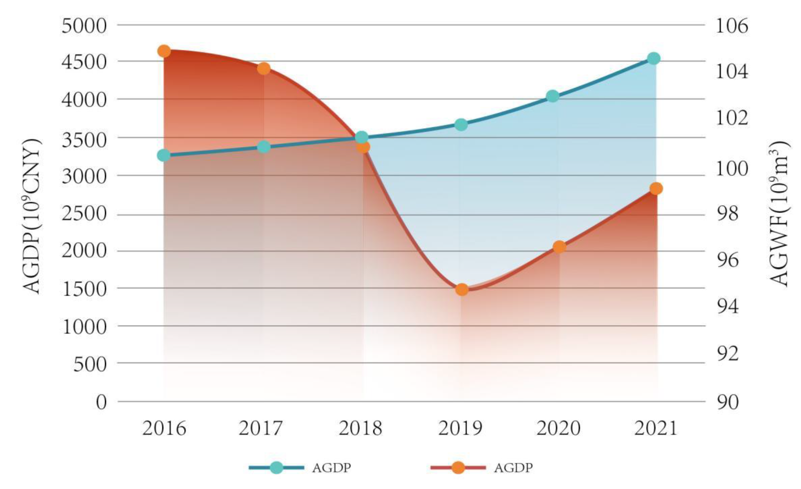
China’s rapid agricultural modernization has been accompanied by continued growth in economic output, water resource use and environmental pressures, and water resources and economic growth are quite related [28]. There are some existing studies that applied the Gini coefficient method, the imbalance index method, and other methods to research the relationship between water resources and the economy [28]. For example, Peng et al. applied the water footprint calculation model VAR and co-integration models in their study to find the correlation between water resources and economic growth [29]. Since water pollution and scarcity significantly impact agricultural economic growth, which can cause environmental damage, it is critical to decouple the agricultural grey water footprint from economic growth [30]. Decoupling theory is a related theory applied to physics to illustrate that the mutual correlation between two or more physical quantities decreases or no longer exists. In 2005, Tapio analyzed the relationship between the transportation sector and GDP from 1970 to 2001, and decoupling elasticity was proposed [31]. The Organization for Economic Co-operation and Development (OECD) first used the decoupling theory to discuss the correlation between environmental quality and economic development [32]. It defined “decoupling” as the rupture of the coupling relationship between ecological quality change and economic progress. It believed that decoupling broke the connection between environmental pressure and financial performance and put forward the conceptions of relative and absolute decoupling. Gradually, scholars began to use Tapio decoupling analysis to discuss the decoupling relationships between water resources, ecological environment and economic progress [1,33,34]. Tao adopted the decoupling theory to study the relationship between water resource utilization and economic development in Beijing [35]. Wang et al. also conducted the decoupling theory to study a decomposition analysis of decoupling from water use and economic growth in 31 regions of China [36]. In addition, the Tapio decoupling model (TDM) was adopted to detect the correlation between carbon emissions and agricultural economic progress [37]. Subsequently, the LMDI method was combined with the TDM to study the relationships between resource reserves, energy and carbon emissions [38,39,40,41]. Few scholars have combined the LMDI and the TDM to conduct in-depth research on the AGWF in the YRB. Kong et al. employed LMDI and TDM to review changes in the water footprint within three provinces of China (Beijing, Tianjin and Hebei) [1]. However, a vast area is covered by the Yellow River Basin (YRB), and the basin faces additional intricate influencing factors.

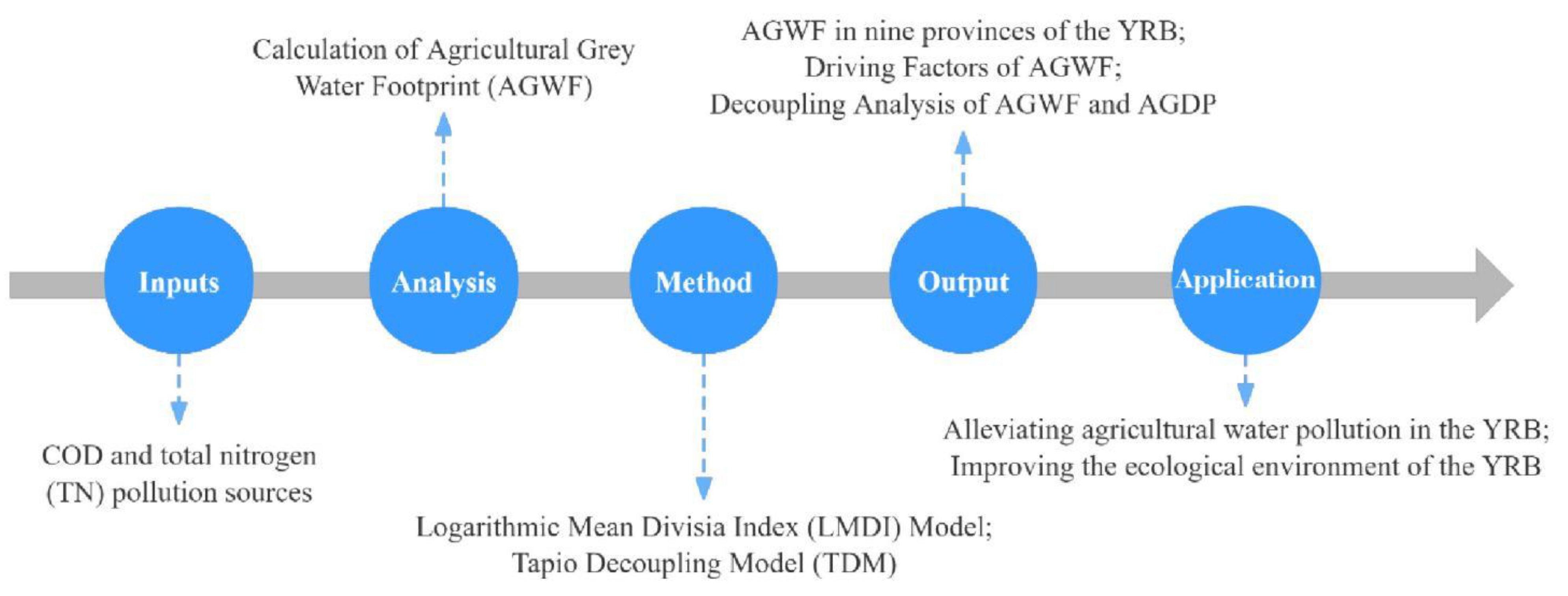
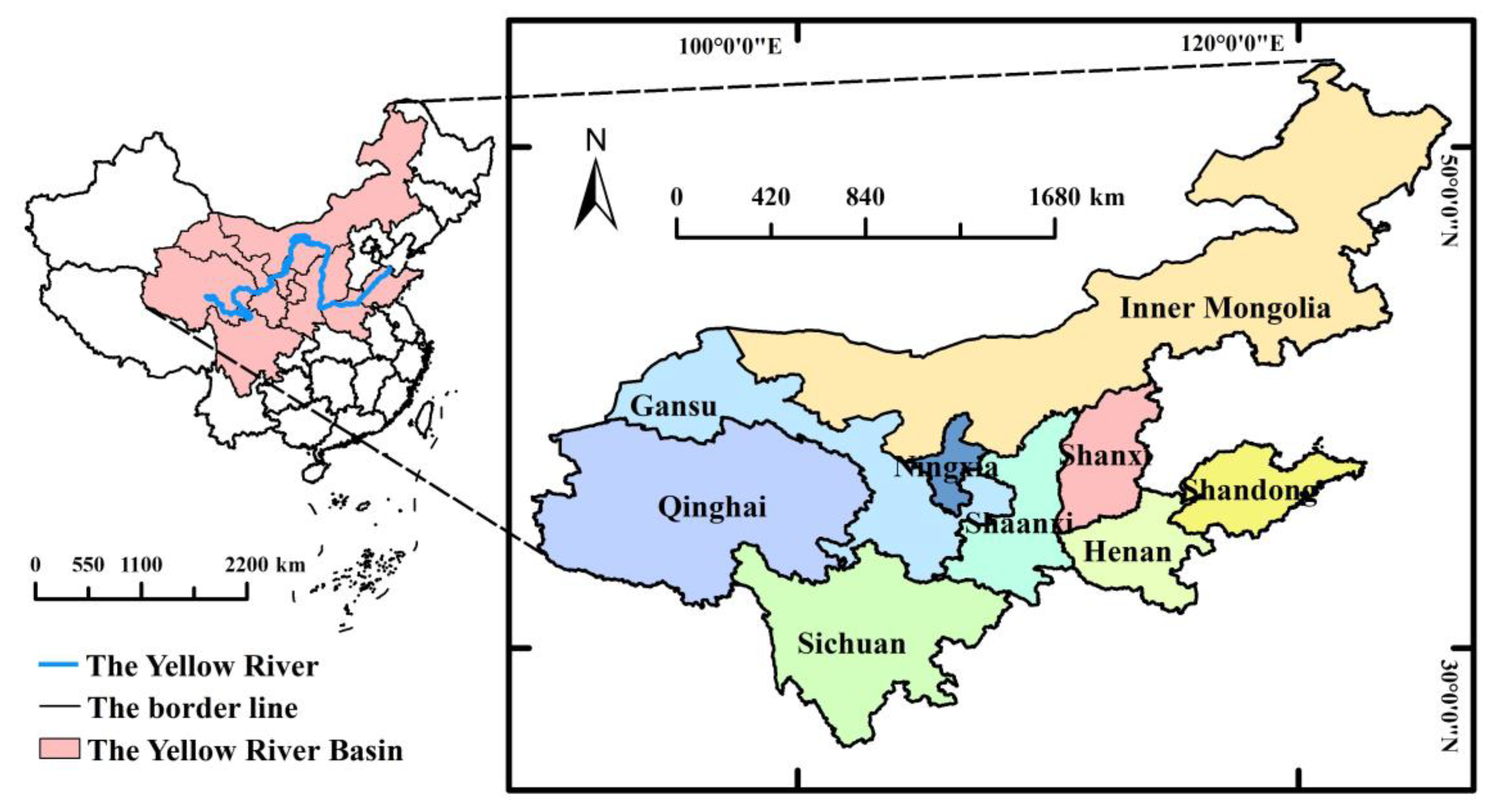
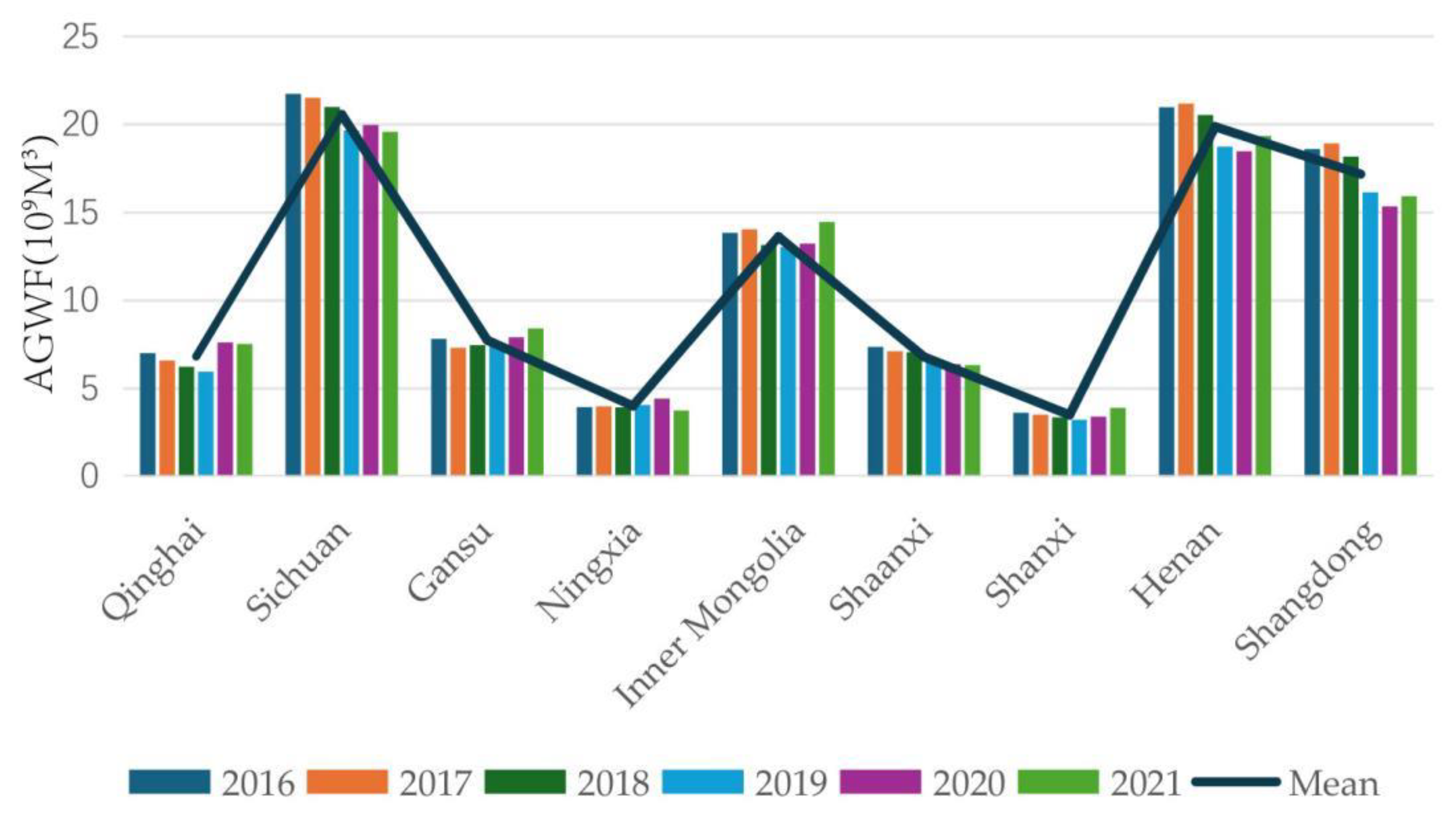
To fill in the research gaps mentioned above, this paper takes the YRB as the research objective and combines the LMDI and TDM to conduct AGWF research in seven provinces and two regions in the YRB. The key contributions of our research include the following points: (1) The AGWF in the YRB during 2016–2021 was accurately estimated via crop farming and animal husbandry, and the trend of the AGWF was evaluated as a whole. (2) The LMDI model was adopted to quantitatively decompose and analyze the driving factors of the AGWF. (3) The TDM was introduced to dissect the decoupling state between the AGWF and AGDP in the YRB, and the decoupling relationship between AGWF driving factors and AGDP was discussed. The rest of this paper is organized as follows: Section 2 introduces the research areas, research approaches and data origins. Section 3 depicts the fundamental discoveries. A deep analysis and discussion regarding essential results are offered in Section 4. Conclusions are shown in Section 5, including main discoveries, suggestions and limitations.

2. Materials and Methods

The overall technical route flowchart of this paper is shown in Figure 1.

2.1. Study Area

The Yellow River is China’s second longest river. It has a length of 5646 km and a drainage area of 79.5 billion m³, occupying roughly 8% of China’s total drainage regions. The YRB spans several provinces, most of which are arid regions and semi-arid regions. The mean annual precipitation of YRB ranges from 123 mm to 1021 mm with an increase from the northwest to the southeast [42]. The Yellow River flows through the following seven provinces and two regions: Qinghai, Sichuan, Gansu, Ningxia Hui Autonomous Region (referred to as Ningxia in the later text), Inner Mongolia Autonomous Region (Referred to as Inner Mongolia in the later text), Shaanxi, Shanxi, Henan and Shandong. The YRB has developed agriculture and flows through several grain production bases, crucial to ensuring China’s food security. In 2021, the agricultural output value reached 2584.8 billion Chinese Yuan (CNY), contributing 33% of China’s AGDP. However, the severe drought problem in the YRB is serious, and water resources have become scarce. Total water resources in the YRB account for roughly 2% of China’s total water resources, and per capita water resources merely obtain 25% of the average. With limited water resources, the YRB irrigates 15% of Chinese cultivated land and feeds 8% of China’s population [43]. Accordingly, agricultural progress in the YRB is over-reliant upon water resources. Additionally, agricultural water use efficiency is low [20]. In 2021, the total quantity of agricultural water within the YRB reached 11,588.4 m³, occupying 66.26% of the total water, and 90% of the agricultural water was utilized to irrigate farmland. Still, only 39% of the farmland was effectively irrigated. At the same time, livestock production and the overuse of fertilizers and pesticides have caused the destruction of water resources in the research area, and low agricultural water use efficiency becomes the norm. In 2022, the productivity coefficients of farmland irrigation water in Shanxi, Sichuan, Qinghai, Inner Mongolia, and Ningxia were 0.543, 0.473, 0.499, 0.543 and 0.535, respectively. Additionally, the coefficients for these provinces and regions were lower than the national average amount of 0.554 [18]. There is a sense of urgency to enhance agricultural water use efficiency and decrease the agricultural grey water footprint of the YRB [44]. A map of the YRB is displayed in Figure 2.

2.2. Methods

2.2.1. Agricultural Grey Water Footprint (AGWF)

To calculate the AGWF, the AGWF generated by farming and breeding should be considered [16,45]. Nitrogen fertilizer used in agriculture is the most critical factor of water pollution. Chemical Oxygen Demand (COD) is a major water pollutant in industrial discharges monitored by the Chinese government, according to publicly available discharge data [46]. The urine and feces produced by sheep, pigs, cattle and poultry include significant quantities of COD and total nitrogen (TN), constituting the primary origin of water pollution from breeding. This paper only considered the TN and COD produced by farming and breeding in the calculation of the AGWF to simplify the calculation process. Likewise, it was assumed that the rearing cycle for pigs and poultry is less than one year and the rearing cycle for cattle and sheep was greater than one year; hence, the year-end slaughter quantity was adopted for pigs and poultry, and the year-end stock quantity was adopted for cattle and sheep. The river flow, utilization patterns, precipitation levels, and climate change in the YRB were variable between the years 2016 and 2021; however, these variables were not employed in the model of the paper and were, therefore, not considered. In this paper, the calculation formulas of the AGWF are referred to as defined in Kong et al. [6].

The specific formulas are listed below:

$$AGW{F}_{pla}=\frac{\mathsf{\partial }\times Appl}{C_{TN,max}-C_{TN,nat}}$$

(1)

$$AGW{F}_{bre}=max(AGW{F}_{bre(COD)},AGW{F}_{bre(TN)})$$

(2)

$$AGW{F}_{bre(i)}=\frac{E{M}_{bre(i)}}{C_{i,max}-C_{i,nat}}$$

(3)

$$E{M}_{bre(i)}={\displaystyle \sum _{a=1}^4{N}_a\times D_a\times (f_a\times p_{af}\times {\beta }_{af}+u_a\times p_{au}\times {\beta }_{au})}$$

(4)

$$AGWF=max[(AGW{F}_{pla}+AGW{F}_{bre(TN)}),AGW{F}_{bre(COD)}]$$

(5)

In Formulas (1)–(5), $AGW{F}_{pla}$ represents the grey water footprint of planting based on TN. $\mathsf{\partial }$ represents the leaching rate of nitrogen fertilizer. $Appl$ represents the application amount of nitrogen fertilizer. $C_{i,max}$ represents the water quality standard concentration of Class $i$ pollutants, and $C_{i,nat}$ represents the natural background concentration of Class $i$ pollutants, which is assumed to be zero. $C_{i,nat}$ for water pollutants is extremely small and non-significant compared to $C_{i,\max }$ [47]. $AGW{F}_{bre}$ represents the grey water footprint of the livestock industry. $AGW{F}_{bre(i)}$ represents the grey water footprint of Class $i$ pollutants (COD, TN). $E{M}_{bre(i)}$ represents the emission of Class $i$ pollutants; $a$ represents pigs, poultry, cattle and sheep; and $N_a$ represents the number of species $a$. $D_a$ represents the feeding period of $a$. $f_a$ and $u_a$ represent the daily excretion and urine volume of $a$. $p_{af}$ represents the content of fecal pollutants per unit of $a$. $p_{au}$ represents the pollutant content in urine per unit of $a$. ${\beta }_{af}$ represents the rate of pollutant loss per unit of feces of $a$. ${\beta }_{au}$ represents the rate of pollutant loss per unit of urine of $a$. $AGWF$ represents the agricultural grey water footprint. Please refer to Appendix A for the specific values of each parameter.

2.2.2. Logarithmic Mean Divisia Index (LMDI) Model

To explore the driving factors of the AGWF, the LMDI model was employed to divide the AGWF into three parts: the AGWF intensity (AGWFI), the agricultural economic development and the population [1]. The formulas of LMDI model are referred to as defined as Kong et al. [1], and they are listed below:

$$AGW{F}_t={\displaystyle \sum _{j}AGW}{F}_{j,t}={\displaystyle \sum _j\frac{AGW{F}_{j,t}}{AGD{P}_{j,t}}}\cdot \frac{AGD{P}_{j,t}}{P_{j,t}}\cdot P_{j,t}={\displaystyle \sum _{j}A}GWF{I}_{j,t}\cdot AE{D}_{j,t}\cdot P_{j,t}$$

(6)

In Equation (6), $AGW{F}_t$ means the AGWF of the YRB during the year $t$. $AGW{F}_{j,t}$ means the AGWF of $j$ province during the year t. $P_{j,t}$ means the permanent population of $j$ province during the year of t. $AGWF{I}_{j,t}$ means the AGWF intensity of $j$ province during the year $t$, indicating the AGWF produced by a unit of AGDP. The agricultural water resource efficiency will be higher if the index is smaller. $AE{D}_{j,t}$ means the per capita AGDP of $j$ province during the year $t$, which denotes the developmental level of the agricultural economy. If the index becomes greater, the influence of agricultural economic development level upon the AGWF will be more significant. $P_{j,t}$ means the population size of $j$ province during the year $t$. According to Equations (7)–(10), the total effect ($\Delta A$) of the AGWF is decomposed into three effects, namely the efficiency effect ($\Delta AGWFI$), agricultural economic effect ($\Delta AED$) and population effect ($\Delta P$).

$$\Delta A=\Delta AGWFI+\Delta AED+\Delta P$$

(7)

$$\Delta AGWFI={\displaystyle \sum _j\frac{AGW{F}_{j,t}-AGW{F}_{j,0}}{\ln AGW{F}_{j,t}-\ln AGW{F}_{j,0}}}\ln \frac{AGWF{I}_{j,t}}{AGWF{I}_{j,0}}$$

(8)

$$\Delta AED={\displaystyle \sum _j\frac{AGW{F}_{j,t}-AGW{F}_{j,0}}{\ln AGW{F}_{j,t}-\ln AGW{F}_{j,0}}}\ln \frac{AE{D}_{j,t}}{AE{D}_{j,0}}$$

(9)

$$\Delta P={\displaystyle \sum _j\frac{AGW{F}_{j,t}-AGW{F}_{j,0}}{\ln AGW{F}_{j,t}-\ln AGW{F}_{j,0}}}\ln \frac{P_{j,t}}{P_{j,0}}$$

(10)

2.2.3. Tapio Decoupling Model (TDM)

The TDM was adopted to measure the degree of decoupling between two variables [31]. The specific formula of TDM is referred to as defined in He et al. [15]:

$$\phi =\frac{G_{t_1}-G_{t_0}}{G_{t_0}}/\frac{E_{t_1}-E_{t_0}}{E_{t_0}}$$

(11)

In Equation (11), $\phi$ represents the decoupling elastic coefficient, $G_t$ represents the AGWF and its driving factors and $E_t$ represents AGDP. The decoupling state can be decomposed into eight categories in

Table 1. Decoupling status classification.

Decoupling State	$\mathit{\phi }$	$\mathbf{\Delta }\mathit{G}$	$\mathbf{\Delta }\mathit{E}$
Strong decoupling (SD)	(−∞, 0)	<0	>0
Weak decoupling (WD)	(0, 0.8)	>0	>0
Recessive decoupling (RD)	(1.2, +∞)	<0	<0
Expansive coupling (EC)	(0.8, 1.2)	>0	>0
Recessive coupling (RC)	(0.8, 1.2)	<0	<0
Expansive negative decoupling (END)	(1.2, +∞)	>0	>0
Weak negative decoupling (WND)	(0, 0.8)	<0	<0
Strong negative decoupling (SND)	(−∞, 0)	>0	<0

in light of the calculated value [48]. Notably, the strong decoupling (SD) is a perfect state, and this indicates that when the AGDP increases, the AGWF decreases. Meanwhile, the strong negative decoupling (SND) is the worst state; additionally, this shows that the agricultural grey water footprint still rises when an economic recession occurs.

2.3. Data Sources

The relevant AGDP information, resident population, fertilizer, pesticide application, livestock, poultry feeding, etc., involved in this research were supplied by the “Statistical Yearbook of China”, the “China Rural Statistical Yearbook”, and the “Water Resources Bulletin”. All of the AGDP data used in this paper were converted, with 2016 taken as the base period. With data from the livestock rearing cycle, pollutant content in defecation and the fecal loss rates of livestock and poultry were supplied by the Technical Report on Pollution Survey and Countermeasures of Large-Scale Livestock and Poultry Farming in China [49]. COD, nitrogen, ammonia emission standards, nitrogen leaching rate, natural background concentration, and other parameters were taken from He et al. [15].

3. Results

3.1. Spatial–Temporal Characteristics of the AGWF in the YRB

The AGWF of the YRB and its seven provinces and two regions for the period 2016–2021 was calculated, as shown in Figure 3, Figure 4 and Figure 5 and

Table 2. The AGWF in the YRB and nine provincial regions from 2016 to 2021 (Unit: 10⁹ m³).

Region	2016	2017	2018	2019	2020	2021	Mean
Qinghai	7.006	6.591	6.226	5.955	7.612	7.528	6.820
Sichuan	21.732	21.507	20.989	19.654	19.967	19.571	20.570
Gansu	7.817	7.303	7.456	7.580	7.900	8.416	7.745
Ningxia	3.931	3.982	3.918	4.066	4.425	3.745	4.011
Inner Mongolia	13.831	14.042	13.147	13.023	13.225	14.463	13.622
Shaanxi	7.359	7.111	7.059	6.570	6.383	6.319	6.800
Shanxi	3.622	3.510	3.358	3.222	3.399	3.897	3.501
Henan	20.969	21.179	20.525	18.742	18.467	19.348	19.872
Shangdong	18.592	18.908	18.166	16.141	15.340	15.923	17.178
YRB	104.858	104.134	100.844	94.953	96.717	99.209	100.119

and

Table 3. The mean ranking of the AGWF of breeding, AGWF of planting and AGWF.

Region	AGWFbre	AGWFpla	AGWF
Qinghai	5	9	6
Sichuan	1	3	1
Gansu	6	7	5
Ningxia	9	6	8
Inner Mongolia	4	4	4
Shaanxi	7	5	7
Shanxi	8	8	9
Henan	3	1	2
Shangdong	2	2	3

(below). The AGWF in the YRB first decreased and then slowly increased during 2016–2021 (Figure 3). In 2016–2019, the AGWF in YRB reduced yearly, reaching its lowest level in 2019, when it decreased by 9.45%. During 2019–2021, the AGWF in the YRB showed a gradual increase of 4.48% compared with 2019. Overall, the AGWF in the YRB cumulatively decreased by 5.649 billion m³ in six years, with a reduction of 5.39%. From the perspective of the changing trend of the AGWF in the planting and breeding sectors during 2016–2021, the AGWF of the planting industry decreased by 9.093 billion m³, which represented a decrease of 23.96%. The AGWF of the breeding industry cumulatively increased by 3.444 billion m³, an increase of 5.15%. Furthermore, the AGWF of plantation was lower than the AGWF of breeding. In 2016, the AGWF in the breeding sector grew to 1.76 times that of the planting sector. By 2021, the ratio between the two rose to 2.44 times. The gap is gradually widening, as can be seen by comparing these two results.

From Table 2 and Figure 4, it can be seen that the AGWFs in five of the seven provinces and two regions in the YRB showed a downward trend during 2016–2021. Among them, Shandong experienced the largest decrease, with a decrease of 14.36% to 2.669 billion m³, and Ningxia experienced the smallest decrease, with a decrease of 4.73% to 0.186 billion m³. The AGWFs of the other four provinces showed an upward trend, among which Gansu had the largest increase of 7.67% and Inner Mongolia had the smallest increase of 4.57%. The difference may be due to the fact that these four provinces are located in the central and western regions of China, where ecological and economic development is slow, agricultural technology is relatively backward, and a high-resource-consuming agricultural development model is preferred.

According to the average AGWF ranking, the top three provinces are Sichuan, Henan and Shandong (Table 3 and Figure 5). The last three on the list are Shaanxi, Shanxi and Ningxia. Combined with the rankings of the breeding AGWF and planting AGWF, Sichuan’s total AGWF and breeding AGWF both ranked first, and its planting AGWF ranked third. Henan’s planting AGWF ranked first. The total amount of AGWF in Shanxi ranked ninth, and the breeding and planting of AGWF ranked eighth. This shows that the AGWF of the breeding industry significantly impacts the total AGWF ranking.

3.2. Analysis of Driving Factors of AGWF

In this study, the LMDI approach was adopted to decompose the AGWF in the YRB into three parts: efficiency effect, agricultural economic effect and population effect. According to Equations (6)–(10), the results are as exhibited in Figure 6 and Figure 7 and

Table 4. The LMDI analysis of AGWF change in the YRB (Unit: 10⁹ m³).

Year	Efficiency Effect	Agriculture Economic Effect	Population Effect	Total Effect
2016–2017	−3.486	2.371	0.465	−0.650
2017–2018	−7.184	3.587	0.235	−3.362
2018–2019	−11.514	5.395	0.228	−5.891
2019–2020	−8.635	10.206	0.193	1.764
2020–2021	−8.570	11.192	−0.131	2.492
Sum	−39.389	32.752	0.990	−5.646

,

Table 5. The LMDI analysis of AGWF change in Qinghai, Sichuan and Gansu (Unit: 10⁹ m³).

Period	Qinghai				Sichuan				Gansu
	Efficiency Effect	Agriculture Economic Effect	Population Effect	Total Effect	Efficiency Effect	Agriculture Economic Effect	Population Effect	Total Effect	Efficiency Effect	Agriculture Economic Effect	Population Effect	Total Effect
2016–2017	−0.736	0.275	0.047	−0.414	−0.660	0.336	0.099	−0.225	−0.899	0.379	0.006	−0.514
2017–2018	−0.809	0.433	0.011	−0.365	−1.239	0.639	0.082	−0.518	−0.311	0.485	−0.021	0.153
2018–2019	−0.939	0.637	0.031	−0.271	−3.205	1.797	0.073	−1.336	−0.496	0.638	−0.018	0.124
2019–2020	0.895	0.728	0.034	1.657	−2.766	3.033	0.047	0.314	−0.633	0.978	−0.025	0.320
2020–2021	−0.902	0.805	0.013	−0.084	−0.751	0.352	0.002	−0.396	−0.823	1.375	−0.036	0.517
Sum	−2.491	2.878	0.136	0.522	−8.622	6.157	0.304	−2.161	−3.163	3.855	−0.093	0.600

,

Table 6. The LMDI analysis of AGWF change in Ningxia, Inner Mongolia and Shaanxi (Unit: 10⁹ m³).

Period	Ningxia				Inner Mongolia				Shaanxi
	Efficiency Effect	Agriculture Economic Effect	Population Effect	Total Effect	Efficiency Effect	Agriculture Economic Effect	Population Effect	Total Effect	Efficiency Effect	Agriculture Economic Effect	Population Effect	Total Effect
2016–2017	−0.114	0.109	0.057	0.052	0.116	0.113	−0.017	0.212	−0.573	0.270	0.056	−0.248
2017–2018	−0.486	0.394	0.028	−0.064	−1.701	0.867	−0.062	−0.895	−0.157	0.056	0.049	−0.053
2018–2019	0.085	0.023	0.039	0.148	−0.936	0.849	−0.038	−0.124	−0.904	0.393	0.022	−0.489
2019–2020	−0.422	0.758	0.024	0.359	−0.968	1.235	−0.065	0.202	−0.705	0.500	0.018	−0.188
2020–2021	−0.996	0.294	0.023	−0.679	−0.064	1.319	−0.017	1.238	−1.122	1.060	−0.002	−0.064
Sum	−1.932	1.577	0.170	−0.185	−3.553	4.384	−0.199	0.632	−3.463	2.278	0.144	−1.041

and

Table 7. The LMDI analysis of AGWF change in Shanxi, Henan and Shandong (Unit: 10⁹ m³).

Period	Shanxi				Henan				Shandong
	Efficiency Effect	Agriculture Economic Effect	Population Effect	Total Effect	Efficiency Effect	Agriculture Economic Effect	Population Effect	Total Effect	Efficiency Effect	Agriculture Economic Effect	Population Effect	Total Effect
2016–2017	−0.084	0.051	−0.004	−0.038	−0.717	0.818	0.110	0.210	0.183	0.021	0.112	0.316
2017–2018	−0.252	0.037	−0.008	−0.223	−0.971	0.244	0.074	−0.654	−1.256	0.433	0.081	−0.742
2018–2019	−0.489	0.358	−0.005	−0.136	−2.113	0.256	0.073	−1.783	−2.518	0.444	0.049	−2.025
2019–2020	−0.399	0.583	−0.007	0.177	−2.011	1.661	0.075	−0.275	−1.624	0.731	0.092	−0.802
2020–2021	0.142	0.365	−0.010	0.497	−2.792	3.783	−0.111	0.881	−1.262	1.838	0.008	0.583
Sum	−1.083	1.394	−0.034	0.277	−8.605	6.762	0.222	−1.621	−6.478	3.466	0.342	−2.669

. According to Table 4, during 2016–2021, the total effect of the AGWF first showed a sharp decline and, subsequently, a slow rise, cumulatively decreasing by 5.647 billion m³ during the six years. The total effect of the AGWF declined yearly from 2016 to 2019, and the maximum reduction was 5.891 billion m³ from 2018 to 2019. The total effect of the AGWF rose slowly year by year in 2019–2021. Additionally, the maximum increase was 2.492 billion m³ during 2020–2021.

From the decomposition effect of the AGWF (Figure 6), the efficiency effect was always negative, and its absolute value first increased and then decreased. This showed that agricultural water use efficiency became the main factor when the AGWF was reduced. A maximum of 11.514 billion m³ reduced the efficiency effect in 2018–2019. The agricultural economic effect was always positive, and the effect increased year by year. The population effect was positive in most years and decreased year by year. The AGWF increase results from a mixture of the agricultural economic effect and the population effect. As the agricultural economic level gradually improves and the population continues to grow, the problem of rural water pollution will continue to rise. However, the cumulative impact of the agricultural economic effect on AGWF growth over the six years 2016–2021 was about 30 times greater than the cumulative impact of the population effect, indicating that the progress of the agricultural economy dominated the AGWF increase.

From the related provinces (Table 5, Table 6 and Table 7 and Figure 7), during the time period of 2016 to 2021, the total effects of the AGWF in Sichuan, Ningxia, Henan and Shandong all decreased, while the full effects of the AGWF in Qinghai, Gansu, Inner Mongolia and Shanxi increased. Among them, the total reduction effects for the AGWF in Shandong, Sichuan and Henan ranked among the top three, with 2.669 billion m³, 2.161 billion m³ and 1.621 billion m³, respectively, contributing significantly to the decrease in the AGWF from 2016 to 2021. The total AGWF effect of Inner Mongolia increased the most, and it was 0.632 billion m³. Via the decomposition effect, the cumulative contribution of the efficiency effect in the seven provinces and two regions was negative, and the incremental contribution from the agricultural economic effect was positive, while the cumulative contribution of the population effect was negative only in Shanxi, Inner Mongolia and Gansu, and the other provinces were positive. The increase or decrease in the AGWF in the seven provinces and two regions was mainly caused by agricultural economic effects or efficiency effects, which were similar to the results in Table 4. It is noteworthy that the cumulative contribution from agricultural economic effects to the AGWF increase in Shandong, Sichuan and Henan ranked fifth, second, and first, respectively. However, the cumulative reduction in the AGWF caused by efficiency effects ranked third, first, and second, respectively, much higher than the cumulative reductions in the AGWF caused by efficiency effects in other provinces. It shows that the agricultural water-saving technology and irrigation technology within three provinces have been prominently enhanced compared to the other six provinces, thus strengthening the agricultural water use efficiency and alleviating the problem of agricultural water pollution.

3.3. Decoupling Analysis of AGWF and AGDP

The changing trend of AGDP and the AGWF in the YRB during 2016–2021 is exhibited in Figure 8. The decoupling state of the AGWF and its decomposition factors from AGDP are displayed in

Table 8. Decoupling status of AGWF and its driving factors and AGDP.

Year	Decoupling Elasticity of AGWF and AGDP	Decoupling Status	Decoupling Elasticity of AGWFI and AGDP	Decoupling Status	Decoupling Elasticity of P and AGDP	Decoupling Status
2017–2018	−1.002195098	SD	33.6473	END	−0.495061127	SD
2018–2019	−1.094079494	SD	11.29061	END	−0.029251404	SD
2019–2020	0.173306378	WD	−2.33237	SD	−0.152678292	SD
2020–2021	0.208439086	WD	−0.06081	SD	−1.675894151	SD

Notes: Green represents strong decoupling; light green indicates weak decoupling; and red indicates expansion negative decoupling.

. The AGDP showed a stable growing trend, while the AGWF showed a changing trend of, firstly, a sharp decline and then a slow rise (Figure 8). According to the data in Table 8, the decoupling states of the AGWF and AGDP were manifested as SD in 2017–2019 and WD in 2019–2021, which conforms to the changing trend in Figure 8. In light of the decoupling relationship between the decomposition factors of the AGWF and AGDP, the decoupling between them was not considered since AGDP and agricultural economic development belong to the economic category. In addition, the AGWFI and AGDP showed END in 2017–2019, followed by SD in 2019–2021. Furthermore, the decoupling state always presented SD between the population effect and AGDP.

Separately, (1) although the decoupling state between the AGWF and AGDP was SD in 2017–2019, from a numerical point of view, the decoupling state of 2018–2019 was higher than that of 2017–2018, while the decoupling state was WD after 2019. The decoupling state gradually became weaker over time, indicating that from 2017 to 2019, with the continuous increase in AGDP, continuous decrease in the AGWF, and the reduction speed becoming faster and faster, the agricultural water pollution problem in the YRB was effectively controlled. From 2019 to 2021, with the continuous increase in AGDP, the AGWF increased. Still, the growth rate of the AGWF was significantly slower than that of AGDP, indicating that the control of agricultural grey water footprint in the YRB was relaxed. (2) The decoupling state between the AGWFI and AGDP showed END in 2017–2019, but the value of 2018–2019 was much lower than that of 2017–2018, indicating that although both were in the END state, the END state gradually decreased with the increase in time. Although the AGWFI increased with the increase in AGDP, and the growth rate of the AGWFI was much higher than that of AGDP, the growth rate of the AGWFI slowed down, indicating that the agricultural water use efficiency in the YRB was not greatly improved, but decision-makers have paid the issue of improving agricultural water use efficiency attention. Although the decoupling state between the AGWFI and AGDP was in SD from 2019 to 2021, the value of 2019–2020 is lower than that of 2020–2021, indicating that the SD state was unstable. This indicates that although the AGWFI decreased with the growth of AGDP during 2019–2021, the rate of AGWFI decline slowed down, that is, agricultural water use efficiency was yet to be steadily improved. (3) The decoupling state between P and AGDP showed SD during 2017–2021, illustrating that with the AGDP increase, the population in the YRB decreased to some degree, that is, the AGDP increase did not depend on population growth. However, the decoupling strength of different stages was different, as the SD state was strongest during 2018–2019 and weakest during 2020–2021.

4. Discussion

4.1. Discussion of AGWF

This paper first calculated and evaluated the 2016–2019 AGWF in the YRB. Subsequently, the LMDI approach was adopted to decompose the AGWF drivers. Next, the decoupling relations were detected among the AGWF, its driving factors, and AGDP growth through the Tapio decoupling model.

This study confirms that the overall AGWF decreased in the YRB, with a downward trend in 2016–2019 and an upward trend in 2019–2021 (Figure 3). Kong et al. also found that China’s AGWF showed a downward trend from 2015 to 2019 [6]. Xu et al. further found that the AGWF of prefecture-level cities in the YRB continued to decline from 2015 to 2019 [50]. The research conclusions of this paper are consistent with those of Kong et al. and Xu et al. [6,50]. The reason why the AGWF in the YRB decreased at first and then rose slowly during 2016–2021 may be that the implementation of the high-quality development strategy in the YRB had a strong promotion effect on reducing the agricultural grey water footprint and improving agricultural water use efficiency in the region in 2016 and for the following three years. However, there was an increase in the AGWF in the YRB between 2019 and 2021, which COVID-19 may have influenced. The impact of COVID-19 may have led to a loosening of controls on agricultural pollutants. This result is consistent with that of Kuttippurath et al., who found that agricultural activities and the use of nitrogen fertilizer increased during the COVID-19 period due to lack of restrictions [51]. To ensure national agricultural security, China’s National Development and Reform Commission put agricultural output in first place in 2020 and temporarily weakened agricultural pollution controls.

This paper found that the AGWF in Qinghai, Shanxi, Gansu and Inner Mongolia increased from 2016 to 2021, mainly due to the severe shortage of water resources in the above four provinces. Wei et al. pointed out that water resource endowment plays a decisive role in alleviating the problem of the agricultural grey water footprint [52]. To promote the rapid development of the agricultural economy, the four provinces mentioned above often used sewage for agricultural irrigation while applying fertilizer in large quantities for a long time. Although sewage irrigation can provide land with a stable water source and bring phosphorus, nitrogen and other chemical elements needed for crops, it inevitably aggravates the problem of agricultural non-point source pollution. In addition, Qinghai, Gansu and Inner Mongolia are major provinces of animal husbandry, and the rapid development of animal husbandry has increased the loads of resources and the environment. This finding is supported by the study of Wen et al., who suggest that the high concentrations of pollutants in the soil have led to the worsening of agricultural water pollution in northern China [53].

The AGWF in the YRB reached its lowest level in 2019, a significant decrease compared with 2016. The reasons may be as follows: On the one hand, the research data in this paper show that the AGWF was greatly affected by $AGW{F}_{bre}$, and the $AGW{F}_{bre}$ in the YRB reached its lowest level in 2019, reaching 63.112 billion m³, while $AGW{F}_{pla}$ decreased year by year. On the other hand, implementing the new development concept in the YRB continued to promote the green transformation of agricultural development. China promulgated the National Water Saving Action Plan and subsequently brought forward a nationwide strategy for the ecological protection and high-quality progress of the YRB in 2019. During the same year, the related provinces responded to the nation’s call and actively launched water-saving action implementation plans aligned with other provinces. With the promotion of various policies, the problem of agricultural water pollution in the YRB has been controlled.

4.2. Discussion of Driving Factors of AGWF

In our study, the driving factors of the AGWF are split into the efficiency effect, agricultural economic effect and population effect by the LMDI model, and the contribution degree of the three decomposition effects to the AGWF are discussed. From 2016 to 2021, the agricultural economic effect was the primary factor driving AGWF increase in the YRB, while the population effect contributed little to the rise in the AGWF, and the efficiency effect was an essential reason for the decrease in the AGWF. The same conclusion can be reached from the relevant provinces. Similarly, it was concluded that the increase or decrease in the grey water footprint was mainly caused by economic or technological effects through the LMDI approach [27]. Moreover, the Generalized Divisia Index Method (GDIM) was adopted to dissect the driving factors of the AGWF in China and Hubei Province, respectively. It was found that agricultural economic growth inhibited the decline of the AGWF, while the AGWFI promoted the AGWF’s decrease [6,15]. Chen et al. analyzed the water resource carrying capacity (WRCC) in the YRB during 2009–2018 through LMDI decomposition and concluded that wastewater treatment technology promoted the WRCC. However, the WRCC was inhibited by the economic effect [54]. The above studies demonstrate that the reduction in the AGWF is mainly promoted by the efficiency effect and inhibited by the agricultural economic effect. The efficiency effect in our research area on AGWF reduction in 2021 increased by 1.5 times compared with that in 2016, suggesting that the planting technology was enhanced, as well as agricultural sewage treatment technology; animal husbandry was transformed into a green development model; and the AGWF was, thus, reduced. This finding is supported by the study of He et al., who suggest that agricultural science and technology improvement could lead to AGWF reduction [15]. The degree of agricultural development in southern China is higher than that in northern China; therefore, it can be inferred that the AGWF in southern China is higher than that in northern China. This is consistent with the research conclusion of Kong et al. [6]. However, Wen et al. found that the upward trend of the AGWF in southern China was significantly lower than that in northern China, possibly due to the higher total water resources and better water quality in southern China, as well as higher agricultural resource utilization efficiency compared with northern China [53].

4.3. Discussion of Decoupling States of AGWF with AGDP

In addition, the TDM was adopted in this study to explore the decoupling relationships between the AGWF, its driving factors, and AGDP during 2016–2021. It is shown that the decoupling states of the AGWF and AGDP presented SD in 2017–2019 and WD in 2019–2021. These two decoupling states indicate that in the AGDP growth process, the AGWF first decreased and then rose slowly, thus achieving sustainable agricultural development to a certain extent [6]. Simultaneously, the AGWFI and AGDP showed END during 2017–2019 and SD during 2019–2021. It is highlighted that agricultural water use efficiency was dramatically improved as agricultural irrigation technology and water-saving technology developed, and the ideal state of the AGWFI decreasing with the AGDP increasing was finally realized. Therefore, when dealing with agricultural grey water, it is imperative to properly handle the correlations between the economy, ecology, and resources based upon the water environment carrying capability, focus upon the influences of AGDP and AGWF intensity upon agricultural water use, and improve agricultural water use efficiency through continuously improving agrarian technology [44,54].

5. Conclusions

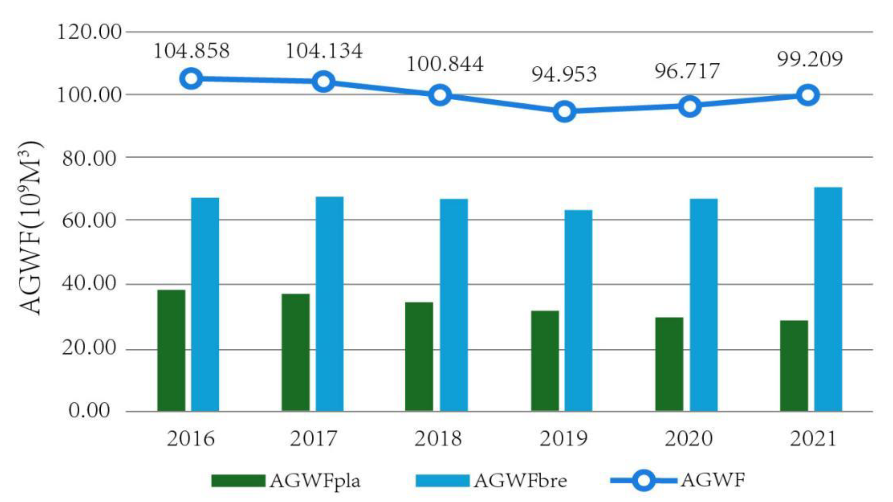
With the sustained and rapid growth of the agricultural economy, the massive application of chemical fertilizers and pesticides and the arbitrary discharge of livestock and poultry manure have aggravated the water pollution of China’s agriculture, seriously restricting the green development of China’s agricultural economy. As an important agricultural region in China, the YRB has a broad plain and fertile soil, which provides unique conditions for China’s agricultural development. This paper provides a method to accurately calculate the AGWF in the YRB during 2016–2021, which can be applied in similar cases in further studies. The LMDI approach was employed to decompose the driving factors that impacted the AGWF. Next, the TDM was adopted to explore the decoupling relationships between the AGWF, its driving factors, and AGDP. The following conclusions were reached:

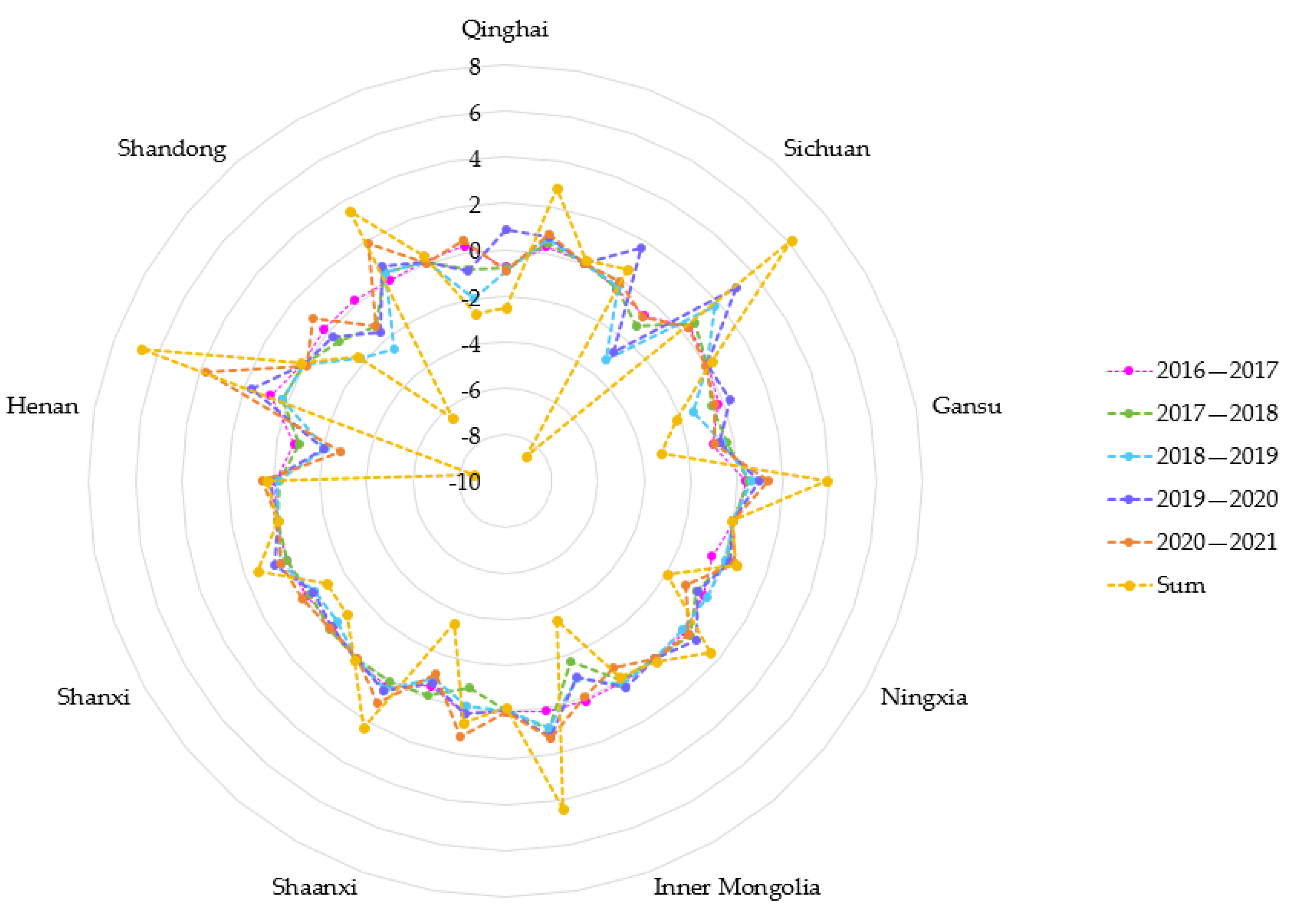
(1) In 2016–2021, the AGWF in the YRB decreased by 5.39%. The AGWF in the research area varied greatly.

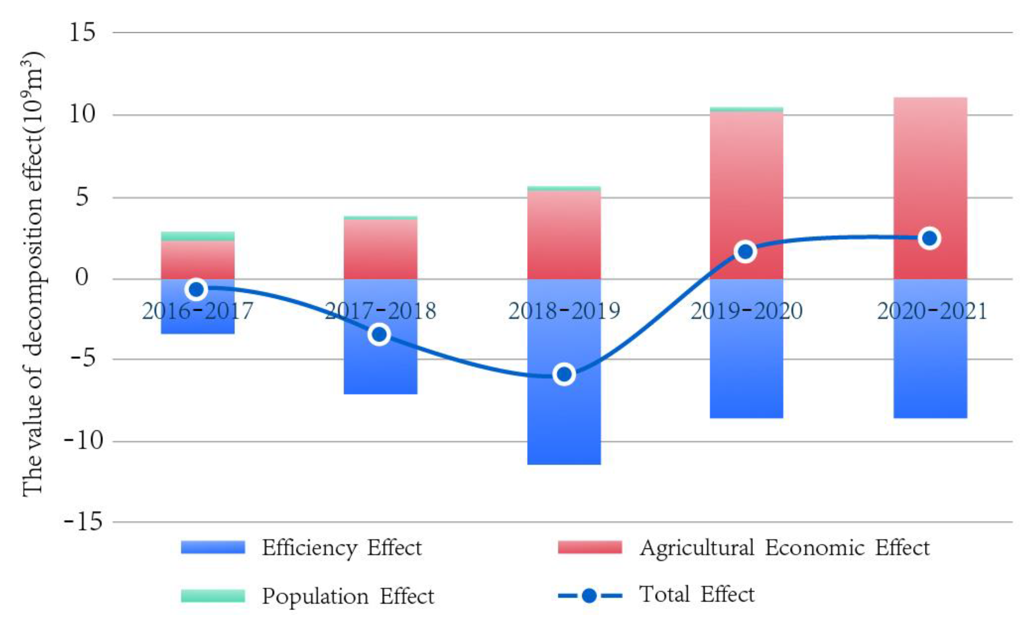
(2) The primary promoting and inhibiting factors of AGWF reduction were the efficiency effect and agricultural economic effect; however, the population effect had a weak inhibiting effect upon AGWF reduction.

(3) Regarding the decoupling states between the AGWF and AGDP, SD and WD were presented first. Moreover, the decoupling state between the AGWFI and AGDP shifted from END to SD. The decoupling between the population and AGDP was in SD. This indicates that agriculture in the research area realized the sustainable development pattern step by step.

Based on the above research conclusions, this paper puts forward the following policy recommendations: (1) Agricultural grey water in different provinces varies greatly; therefore, agricultural water management policies should be formulated according to local conditions, rational allocation of resources and coordinated regional development. (2) It is also vital to constantly improve various infrastructure, accelerate the diversified development of the agricultural economy, cultivate and expand characteristic industries and achieve sustained progress in the agricultural economy. (3) Finally, policymakers should strengthen the protection and scientific and rational use of water resources, further promote the application of water-saving technologies, accelerate the development of green agricultural technologies, consolidate and improve coordination between the agricultural economy and agricultural water use, and achieve the high-quality development of green agriculture.

Although the AGWF in the YRB was measured and analyzed, as were its driving factors, some areas are still worth improving. The generalization of these results is subject to certain limitations. For instance, (1) on account of the challenges of attaining some information related to agricultural grey water, only COD and TN pollution sources were considered in the calculation of the AGWF in this paper, and there may be specific differences between the calculation results of the AGWF and the actual situation of agricultural water pollution. (2) The dynamic evolutionary path between the AGWF and its drivers and AGDP is worth further exploration. (3) Due to time constraints, this paper did not study how the COVID-19 pandemic influenced agricultural pollutants, and this could be further explored.

References

1. Kong, Y.; He, W.; Yuan, L.; Shen, J.; An, M.; Degefu, D.M.; Gao, X.; Zhang, Z.; Sun, F.; Wan, Z. Decoupling analysis of water footprint and economic growth: A case study of Beijing–Tianjin–Hebei Region from 2004 to 2017. Int. J. Environ. Res. Public Health 2019, 16, 4873. [Google Scholar] [CrossRef] [PubMed]
2. Bilge Ozturk, G.; Ozenen Kavlak, M.; Cabuk, S.N.; Cabuk, A.; Cetin, M. Estimation of the water footprint of kiwifruit: In the areas transferred from hazelnut to kiwi. Environ. Sci. Pollut. Res. 2022, 29, 73171–73180. [Google Scholar] [CrossRef] [PubMed]
3. Peng, Q.; He, W.; Kong, Y.; Yuan, L.; Degefu, D.M.; An, M.; Zeng, Y. Identifying the decoupling pathways of water resource liability and economic growth: A case study of the Yangtze River Economic Belt, China. Environ. Sci. Pollut. Res. 2022, 29, 55775–55789. [Google Scholar] [CrossRef] [PubMed]
4. Gosling, S.N.; Arnell, N.W. A global assessment of the impact of climate change on water scarcity. Clim. Chang. 2016, 134, 371–385. [Google Scholar] [CrossRef]
5. Zhang, P.; Yang, D.; Zhang, Y.; Li, Y.; Liu, Y.; Cen, Y.; Zhang, W.; Geng, W.; Rong, T.; Liu, Y. Re-examining the drive forces of China’s industrial wastewater pollution based on GWR model at provincial level. J. Clean. Prod. 2020, 262, 121309. [Google Scholar] [CrossRef]
6. Kong, Y.; He, W.; Zhang, Z.; Shen, J.; Yuan, L.; Gao, X.; An, M.; Ramsey, T.S. Spatial-temporal variation and driving factors decomposition of agricultural grey water footprint in China. J. Environ. Manag. 2022, 318, 115601. [Google Scholar] [CrossRef] [PubMed]
7. Baccour, S.; Albiac, J.; Kahil, T.; Esteban, E.; Crespo, D.; Dinar, A. Hydroeconomic modeling for assessing water scarcity and agricultural pollution abatement policies in the Ebro River Basin, Spain. J. Clean. Prod. 2021, 327, 129459. [Google Scholar] [CrossRef]
8. Mekonnen, M.M.; Hoekstra, A.Y. Global gray water footprint and water pollution levels related to anthropogenic nitrogen loads to fresh water. Environ. Sci. Technol. 2015, 49, 12860–12868. [Google Scholar] [CrossRef]
9. Mekonnen, M.M.; Hoekstra, A.Y. Global anthropogenic phosphorus loads to freshwater and associated grey water footprints and water pollution levels: A high-resolution global study. Water Resour. Res. 2018, 54, 345–358. [Google Scholar] [CrossRef]
10. Xu, R.; Cai, Y.; Wang, X.; Li, C.; Liu, Q.; Yang, Z. Agricultural nitrogen flow in a reservoir watershed and its implications for water pollution mitigation. J. Clean. Prod. 2020, 267, 122034. [Google Scholar] [CrossRef]
11. Xiao, L.; Liu, J.; Ge, J. Dynamic game in agriculture and industry cross-sectoral water pollution governance in developing countries. Agric. Water Manag. 2021, 243, 106417. [Google Scholar] [CrossRef]
12. Huang, J.; Yang, G. Understanding recent challenges and new food policy in China. Glob. Food Secur. 2017, 12, 119–126. [Google Scholar] [CrossRef]
13. Evans, A.E.; Mateo-Sagasta, J.; Qadir, M.; Boelee, E.; Ippolito, A. Agricultural water pollution: Key knowledge gaps and research needs. Curr. Opin. Environ. Sustain. 2019, 36, 20–27. [Google Scholar] [CrossRef]
14. West, P.C.; Gerber, J.S.; Engstrom, P.M.; Mueller, N.D.; Brauman, K.A.; Carlson, K.M.; Cassidy, E.S.; Johnston, M.; MacDonald, G.K.; Ray, D.K. Leverage points for improving global food security and the environment. Science 2014, 345, 325–328. [Google Scholar] [CrossRef] [PubMed]
15. He, W.; Zhang, K.; Kong, Y.; Yuan, L.; Peng, Q.; Degefu, D.M.; Ramsey, T.S.; Meng, X. Reduction pathways identification of agricultural water pollution in Hubei Province, China. Ecol. Indic. 2023, 153, 110464. [Google Scholar] [CrossRef]
16. Hoekstra, A.Y. The Water Footprint Assessment Manual: Setting the Global Standard; Routledge: London, UK, 2011. [Google Scholar]
17. Çankaya, S. Evaluation of the impact of water reclamation on blue and grey water footprint in a municipal wastewater treatment plant. Sci. Total Environ. 2023, 903, 166196. [Google Scholar] [CrossRef] [PubMed]
18. Cheng, P.; Sun, M. Calculation of seasonal agricultural grey water footprint in monsoon region based on river reference conditions. Ecol. Indic. 2022, 145, 109638. [Google Scholar] [CrossRef]
19. Wang, C.; Zhang, H.; Xin, X.; Li, J.; Jia, H.; Wen, L.; Yin, W. Water level–driven agricultural nonpoint source pollution dominated the ammonia variation in China’s second largest reservoir. Environ. Res. 2022, 215, 114367. [Google Scholar] [CrossRef] [PubMed]
20. Zhang, C.; Qiao, H.; Ma, Y.; Wu, C.; Wang, Y.; Huang, B.; Guo, F. Promoting Integrated Management of Water Resources to Ensure High-level Protection and High-quality Developmen. Bull. Chin. Acad. Sci. 2021, 36, 1307–1315. [Google Scholar] [CrossRef]
21. De Girolamo, A.M.; Miscioscia, P.; Politi, T.; Barca, E. Improving grey water footprint assessment: Accounting for uncertainty. Ecol. Indic. 2019, 102, 822–833. [Google Scholar] [CrossRef]
22. Rong, Q.; Wu, H.; Otkur, A.; Yue, W.; Su, M. A novel uncertainty analysis method to improve the accuracy of agricultural grey water footprint evaluation considering the influence of production conditions. Ecol. Indic. 2023, 154, 110641. [Google Scholar] [CrossRef]
23. Hu, J.; Chi, L.; Xing, L.; Meng, H.; Zhu, M.; Zhang, J.; Wu, J. Decomposing the decoupling relationship between energy consumption and economic growth in China’s agricultural sector. Sci. Total Environ. 2023, 873, 162323. [Google Scholar] [CrossRef] [PubMed]
24. Pıša, V.; Bruha, J. The Decomposition Model of the World Agricultural Production and Consumption. 2011. Available online: https://www2.humusoft.cz/www/papers/tcp11/095_pisa.pdf (accessed on 19 January 2024).
25. Gao, Z.; Wang, Y. The decomposition analysis of change of energy consumption for production in China. Stat. Res. 2007, 4, 52–57. [Google Scholar]
26. Zhang, S.; Su, X.; Singh, V.P.; Ayantobo, O.O.; Xie, J. Logarithmic Mean Divisia Index (LMDI) decomposition analysis of changes in agricultural water use: A case study of the middle reaches of the Heihe River basin, China. Agric. Water Manag. 2018, 208, 422–430. [Google Scholar] [CrossRef]
27. Chen, J.; Gao, Y.; Qian, H.; Jia, H.; Zhang, Q. Insights into water sustainability from a grey water footprint perspective in an irrigated region of the Yellow River Basin. J. Clean. Prod. 2021, 316, 128329. [Google Scholar] [CrossRef]
28. Shi, J. Study on the Decoupling Relationship and Rebound Effect between Agricultural Economic Growth and Water Footprint: A Case of Yangling Agricultural Demonstration Zone, China. Water 2022, 14, 991. [Google Scholar] [CrossRef]
29. Peng, W.; Tian, Y. Empirical research on environmental pollution and economic growth in Hunan Province—Based on impulse response function of VAR model. J. Xiangtan Univ. Philos. Soc. Sci 2011, 35, 31–35. [Google Scholar]
30. Yang, Y.; Liu, Y. Spatio-temporal analysis of urbanization and land and water resources efficiency of oasis cities in Tarim River Basin. J. Geogr. Sci. 2014, 24, 509–525. [Google Scholar] [CrossRef]
31. Tapio, P. Towards a theory of decoupling: Degrees of decoupling in the EU and the case of road traffic in Finland between 1970 and 2001. Transp. Policy 2005, 12, 137–151. [Google Scholar] [CrossRef]
32. Linster, M. OECD Environmental Indicators: Development, Measurement and Use. 2003. Available online: https://www.oecd.org/environment/indicators-modelling-outlooks/24993546.pdf (accessed on 20 January 2024).
33. Duan, T.; Feng, J.; Zhou, Y.; Chang, X.; Li, Y. Systematic evaluation of management measure effects on the water environment based on the DPSIR-Tapio decoupling model: A case study in the Chaohu Lake watershed, China. Sci. Total Environ. 2021, 801, 149528. [Google Scholar] [CrossRef]
34. Qin, X.; Hu, X.; Xia, W. Investigating the dynamic decoupling relationship between regional social economy and lake water environment: The application of DPSIR-Extended Tapio decoupling model. J. Environ. Manag. 2023, 345, 118926. [Google Scholar] [CrossRef]
35. Tao, A. Study on the relationship between water resources utilization and economic development based on decoupling theory in Beijing. IOP Conf. Ser. Earth Environ. Sci. 2021, 687, 012207. [Google Scholar] [CrossRef]
36. Wang, Q.; Wang, X. Moving to economic growth without water demand growth—A decomposition analysis of decoupling from economic growth and water use in 31 provinces of China. Sci. Total Environ. 2020, 726, 138362. [Google Scholar] [CrossRef] [PubMed]
37. Wei, Z.; Wei, K.; Liu, J.; Zhou, Y. The relationship between agricultural and animal husbandry economic development and carbon emissions in Henan Province, the analysis of factors affecting carbon emissions, and carbon emissions prediction. Mar. Pollut. Bull. 2023, 193, 115134. [Google Scholar] [CrossRef]
38. Bianco, V.; Cascetta, F.; Nardini, S. Analysis of the carbon emissions trend in European Union. A decomposition and decoupling approach. Sci. Total Environ. 2024, 909, 168528. [Google Scholar] [CrossRef]
39. Dai, T.; Yue, Z. The evolution and decoupling of in-use stocks in Beijing. Ecol. Econ. 2023, 203, 107606. [Google Scholar] [CrossRef]
40. Horoshko, O.-I.; Horoshko, A.; Bilyuga, S.; Horoshko, V. Theoretical and methodological bases of the study of the impact of digital economy on world policy in 21 century. Technol. Forecast. Soc. Chang. 2021, 166, 120640. [Google Scholar] [CrossRef]
41. Yue, X.; Byrne, J. Identifying the determinants of carbon emissions of individual airlines around the world. J. Air Transp. Manag. 2024, 115, 102521. [Google Scholar] [CrossRef]
42. Omer, A.; Zhuguo, M.; Zheng, Z.; Saleem, F. Natural and anthropogenic influences on the recent droughts in Yellow River Basin, China. Sci. Total Environ. 2020, 704, 135428. [Google Scholar] [CrossRef]
43. Jia, S.; Liang, Y. Suggestions for strategic allocation of the Yellow River water resources under the new situation. Resour. Sci 2020, 42, 29–36. [Google Scholar] [CrossRef]
44. Lu, C.; Ji, W.; Hou, M.; Ma, T.; Mao, J. Evaluation of efficiency and resilience of agricultural water resources system in the Yellow River Basin, China. Agric. Water Manag. 2022, 266, 107605. [Google Scholar] [CrossRef]
45. Han, Q.; Sun, C.; Zou, W. Grey water footprint efficiency measure and its driving pattern analysis on provincial scale in China from 1998 to 2012. Resour. Sci 2016, 38, 1179–1191. [Google Scholar] [CrossRef]
46. Liu, A.; Han, A.; Chai, L. Life cycle blue and grey water in the supply chain of china’s apparel manufacturing. Processes 2021, 9, 1212. [Google Scholar] [CrossRef]
47. Su, Y.; Liang, Y.; Chai, L.; Han, Z.; Ma, S.; Lyu, J.; Li, Z.; Yang, L. Water degradation by China’s fossil fuels production: A life cycle assessment based on an input–output model. Sustainability 2019, 11, 4130. [Google Scholar] [CrossRef]
48. Kong, Y.; He, W.; Yuan, L.; Zhang, Z.; Gao, X.; Degefu, D.M. Decoupling economic growth from water consumption in the Yangtze River Economic Belt, China. Ecol. Indic. 2021, 123, 107344. [Google Scholar] [CrossRef]
49. CEPA. Investigation and Countermeasures on Pollution of Large-Scale Livestock and Poultry Industry in China; China Environmental Science Press: Beijing, China, 2002. [Google Scholar]
50. Xu, R.; Shi, J.; Hao, D.; Ding, Y.; Gao, J. Research on Temporal and Spatial Differentiation and Impact Paths of Agricultural Grey Water Footprints in the Yellow River Basin. Water 2022, 14, 2759. [Google Scholar] [CrossRef]
51. Kuttippurath, J.; Patel, V.; Kashyap, R.; Singh, A.; Clerbaux, C. Anomalous increase in global atmospheric ammonia during COVID-19 lockdown: Need for policies to curb agricultural emissions. J. Clean. Prod. 2023, 434, 140424. [Google Scholar] [CrossRef]
52. Wei, J.; Lei, Y.; Yao, H.; Ge, J.; Wu, S.; Liu, L. Estimation and influencing factors of agricultural water efficiency in the Yellow River basin, China. J. Clean. Prod. 2021, 308, 127249. [Google Scholar] [CrossRef]
53. Wen, L.; Lei, M.; Zhang, B.; Kong, X.; Liao, Y.; Chen, W. Significant increase in gray water footprint enhanced the degradation risk of cropland system in China since 1990. J. Clean. Prod. 2023, 423, 138715. [Google Scholar] [CrossRef]
54. Chen, Q.; Zhu, M.; Zhang, C.; Zhou, Q. The driving effect of spatial-temporal difference of water resources carrying capacity in the Yellow River Basin. J. Clean. Prod. 2023, 388, 135709. [Google Scholar] [CrossRef]
Figure 1. Technical route flowchart.
Water 16 01129 g001
Figure 2. Map of the Yellow River Basin (YRB).
Water 16 01129 g002
Figure 3. AGWF, AGWF of planting and AGWF of breeding in YRB.
Water 16 01129 g003
Figure 4. The AGWF of the nine provinces and regions in the YRB from 2016 to 2021.
Water 16 01129 g004
Figure 5. The mean rankings of the AGWF of breeding, AGWF of planting and AGWF.
Water 16 01129 g005
Figure 6. The changing trend of the AGWF of the YRB LMDI decomposition effect.
Water 16 01129 g006
Figure 7. The LMDI analysis of AGWF change in seven provinces and two regions in the YRB.
Water 16 01129 g007
Figure 8. The changing trend of the AGWF and AGDP in the YRB (2016–2021).
Water 16 01129 g008