Research on Permeability Characteristics and Gradation of Rockfill Material Based on Machine Learning

Abstract

The density of rockfill material is an important index to evaluate the quality of rockfill dams. It is of great significance to accurately obtain the densities and permeability coefficients of rockfill material dams quickly and accurately by scientific means. However, it takes a long time to measure the permeability coefficient of rockfill material in practice, which means that such measurements cannot fully reflect all the relevant properties. In this paper, using a convolutional neural network (CNN), a machine learning model was established to predict the permeability coefficient of rockfill material with the full scale (d₁₀~d₁₀₀), pore ratio, Cu, and Cc as the inputs and the permeability coefficient as the output. Through collecting the permeability coefficient and related data in the literature, the set samples were sorted for model training. The prediction results of the trained CNN model are compared with those of the back propagation (BP) model to verify the accuracy of the CNN model. Laboratory constant head penetration experiments were designed to verify the generalization performance of the model. The results show that compared with the BP model, the CNN model has better applicability to the prediction of the permeability coefficient of rockfill material and that the CNN can obtain better accuracy and meet the requirements of the rough estimation of rockfill materials’ permeability in engineering.

1. Introduction

As an important part of the national infrastructure, the water conservancy project is vital to the sustainable development of agricultural production, urban water supply, ecological environment protection, and other fields. The water conservancy dam is a crucial structure in water conservancy projects, and its safety is directly related to the national economic construction, improvements in the lives of the people, and the protection of the ecological environment. In recent years, with the rapid development of national water conservancies, higher requirements have been put forward for dam quality monitoring. In rockfill material dam projects, the construction quality of the rockfill material for dam building is the most important aspect of the overall dam quality control. The quality of the rockfill material in dams directly affects the safety of the construction and operation of the project, and it is crucial to the long-term development of water conservancy. The main factor affecting the quality of rockfill material dams is the compaction quality, and the main control index of compaction quality is the density of the rockfill material. Therefore, an appropriate scientific method to study and control the density of rockfill material is needed. For rockfill material dams, the main indicators of dam construction quality include density, particle gradation, and permeability characteristics. The focus in the current construction is to monitor these data quickly and accurately by developing effective methods. It is crucial to monitor these data to control the compaction quality and the safety of the dam. Therefore, in the field of water conservancy engineering, the continuous improvement of the methods for monitoring the quality of dam construction, effective control, and the monitoring of dam quality indicators through scientific methods are important ensure the safe operation of water conservancy projects.

In the past, permeability characteristic and permeability coefficient studies of dams were mainly carried out in laboratories or in the field. The field tests mainly included the trail pit seepage test and drilling grouting test, while the laboratory tests mainly included the constant head permeability test and the model seepage test. However, field tests have some disadvantages, such as their time-consuming processes, small monitoring range, and low monitoring efficiency. For their part, laboratory tests also have certain limitations. The actual working conditions may not be accurately reflected and the permeability coefficient data might not be obtained promptly [1]. Some scholars have proposed empirical formulae for estimating the permeability coefficient, including the Terzaghi [2] formula:

$$K=2d_{10}^2{e}^2$$

(1)

and Kozeny’s formula:

$$K_{18}=780\frac{n^3}{{\left(1-n\right)}^2}{d}_9^2$$

(2)

where e is the pore ratio, n is the porosity, and d_m is the effective particle size of each corresponding formula.

However, the use of empirical formulae to estimate the permeability coefficients of rockfill materials is often inconsistent with the actual situation because these empirical formulae cannot comprehensively take into account the influence of various factors. , Thus, empirical formulae have a limited scope of application [3]. The coefficient of permeability of coarse-grained soil is affected by many factors, such as the dry density [4], particle shape [5,6], fine content [7,8], coefficient of uniformity [9,10], and pore ratio [11,12]. Chapuis [13] proposed a new equation to predict the saturated hydraulic conductivity of sand and gravel using the effective diameter and void ratio, finding that the new equation predictions were usually between 0.5 and 2.0 times the measured value for the considered data using the values of d₁₀ and e. Koohmishi [14] conducted a laboratory test on a coarse aggregate to evaluate the effect of gradation and compaction on permeability and found that gradation is the property that most affects permeability. Dolzyk et al. [15] proposed a relationship between the void ratio, the coefficient of uniformity, and the effective size and the coefficient of permeability.

Due to the development of artificial intelligence, some scholars began to use artificial neural network methods to predict the permeability coefficient [16,17,18,19]. Yilmaz et al. [20] predicted the permeability coefficients of coarse-grained soils by using neural networks and compared and analyzed different prediction models, which provided a new methodology and approach for obtaining the permeability coefficients of soils. Zhang et al. [21] developed a predictive equation of the permeability characteristics of soil using gene expression programming (GEP) and conducted a sensitivity analysis, including the effective size (d₁₀), mean grain size (d₅₀), and void ratio (e). Al Khalifah et al. [22] used two machine learning techniques to predict the permeability of carbonate rock and compared them with seven conventional methods, finding that machine learning performed better than all the conventional empirical methods, especially neural networks.

The factors influencing the permeability coefficient are complex in rockfill material. The neural network model has more input parameters, and less research has been conducted on predicting permeability coefficients with convolutional neural network (CNN) models. In recent years, with the development of machine learning technology, CNNs have gradually received increasing attention. With their special architecture and powerful feature analysis and processing ability, CNNs can more easily handle multi-dimensional data, such as the particle gradation and permeability coefficient, in the field of rockfill materials, and they extract the features of these materials for fitting predictions to improve the accuracy. Therefore, in this paper, a CNN was used to build a machine learning model, and a BP neural network was also built to make contrastive analysis. In addition, the applicability of the CNN in the prediction of the permeability coefficient of rockfill material was verified through a laboratory permeability test.

2. CNN Predictive Models

CNNs are well known for their excellent feature extraction capabilities in image processing, but they are equally suitable for processing other types of data, including one-dimensional data. Even though our data are one-dimensional, there are still local correlations and structural features. CNNs are able to capture these features efficiently and are effective tools for working with one-dimensional sequential data. CNNs are able to extract important local patterns and global structure from the data, which makes the model’s representation of the data more efficient and accurate.

2.1. Basic Principle of Convolutional Neural Network

The CNN is a kind of deep feed-forward neural network with local connection, weight sharing, and other characteristics. As one of the representative algorithms of machine learning, it is good at dealing with images, especially image recognition and other related machine learning problems, and it can also be used in data regression prediction. CNNs have representational learning capabilities and are able to classify input information according to its hierarchical structure in a translation-invariant way, allowing both supervised and unsupervised learning [23]. Compared with traditional neural networks, CNNs have the following advantages. They can automatically learn the features in the data instead of designing the features manually, which makes them more efficient and flexible in dealing with large-scale data. In addition, CNNs can capture local features in data and extract more abstract and important features through pooling operations. Moreover, CNNs can construct deep networks by stacking multiple convolutional and fully connected layers to further improve performance.

2.2. CNN-Model Structure

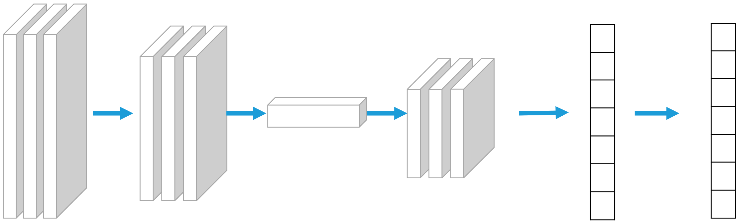
The CNN is divided into a 3-layer structure: input layer, hidden layer, and output layer. The input layer is responsible for importing data. The hidden layer includes convolutional layer, pooling layer, and fully connected layer. The convolutional layer uses convolutional operations to extract features from the input data. It consists of multiple convolution kernels and each convolution kernel detects features of the input data, such as edges and texture. The convolution operation is computed on the input data by sliding filters to generate a feature map as input to the next layer. The pooling layer is responsible for down-sampling the feature map output from the convolutional layer to reduce the computation by retaining the maximum and average values in the region. The pooling layer helps to reduce the size of the feature map while retaining the key features. The fully connected layer is usually located at the end of the network and its nodes are connected to all the nodes in the previous layer. The fully connected layer transforms the features extracted from the pooling layer into the final output by combining and learning the features and producing the final output. The output layer is responsible for receiving signals from the fully connected layer and generating the output predicted by the model [24]. Therefore, to make the model fit the dataset better and improve the prediction accuracy, the convolutional layer–pooling layer–convolutional layer structure is designed so that the model is convolved once, pooled, and then convolved again to make the model obtain more features for fitting learning. The structure is shown in Figure 1.

2.3. Model Construction

For the permeability-coefficient-prediction task, the input data are a one-dimensional array containing permeability-related features, including gradation, inhomogeneity coefficients, pore ratios, and curvature coefficients, as well as the permeability coefficient. In this paper, MATLAB-R2022a is used to construct a CNN [25]. The specific steps are as follows:

(1) Data input. The dataset was imported in the form of an Excel table and divided into the training set and test set.

(2) Data preprocessing. To ensure that the dataset allows the model to identify and learn features, it is necessary to preprocess the input data, and the specific steps include normalization and data tiling. Normalization is used to change all the data to the (0, 1) interval, using the function mapminmax. Data tiling is used because the CNN is mainly used for image processing; the images are generally in three dimensions, and they need to be converted to one dimension to ensure that the dimensionality of the data and the dimensionality of the input layer of the model are consistent. The following is the mapminmax function:

$$y=\frac{(y_{\max }-y_{\min })\times (x-x_{\min })}{x_{\max }-x_{\min }}+y_{\min }$$

(3)

where $x$ is the original data, $x_{\min }$ and $x_{\max }$ are the minimum and maximum values of the original data, respectively, $y_{\min }$ and $y_{\max }$ are the minimum and maximum values of the target range, respectively, and $y$ is the normalized data.

(3) The network structure construction, building convolutional, pooling, and fully connected layers. First, the neural network’s input layer is created using the imageInputLayer function, and the input-data dimension is set to [13, 1, 1], which corresponds to d₁₀~d₁₀₀, e, C_u, and C_c, respectively. Next, the convolution layer is constructed using the Convolution2D function, and the size of the convolution kernel is 3 × 1. The pooling layer is constructed by the MaxPooling2D function, setting the pooling window to [2, 1] and the step size to [1, 1]. After the pooling layer, the same convolutional layer with the same convolutional kernel is set, and the size of feature map is adjusted to 32. The Dropout function is used to introduce the regularization technique, and the parameter size of the L2Regularization function is set to 0.01, in order to reduce the risk of overfitting and the effect of multicollinearity of the input features. Finally, the fullyConnectedLayer and Regression functions are used to construct the fully connected layer and the regression layer, respectively. The Activation function between layers uses the ReLU function to improve the nonlinear fitting ability of the model in the following form:

$$f(x)=\max (0,x)$$

(4)

(4) Model training hyperparameter settings. Suitable parameters would allow better model fitting, less training time, and better prediction accuracy. The maximum number of model training is set to 1200. The number of samples per training is 30. The initial learning rate is 0.01, and the learning rate’s decrease factor is 0.5. The SGDM function is chosen as the optimization function, which serves to minimize the loss function by calculating the gradient of each parameter and updating the parameters using momentum, which can help the neural network to converge to the optimal solution more quickly while reducing the oscillations when the parameters are updated. Its expression function is as follows:

$$v_{\mathrm{t}+1}=\beta v_{\mathrm{t}}+(1-\beta )\nabla J({\theta }_{\mathrm{t}})$$

(5)

$${\theta }_{\mathrm{t}+1}={\theta }_{\mathrm{t}}-\alpha v_{\mathrm{t}+1}$$

(6)

where ${\theta }_{\mathrm{t}+1}$ and ${\theta }_{\mathrm{t}}$ are the model parameters before and after updating, respectively, $\nabla J({\theta }_{\mathrm{t}})$ is the parameter gradient, $\alpha$ is the learning rate, $v_{\mathrm{t}}$ and $v_{\mathrm{t}+1}$ are the momentum before and after updating, respectively, and $\beta$ is the momentum parameter, which takes a value between 0 and 1.

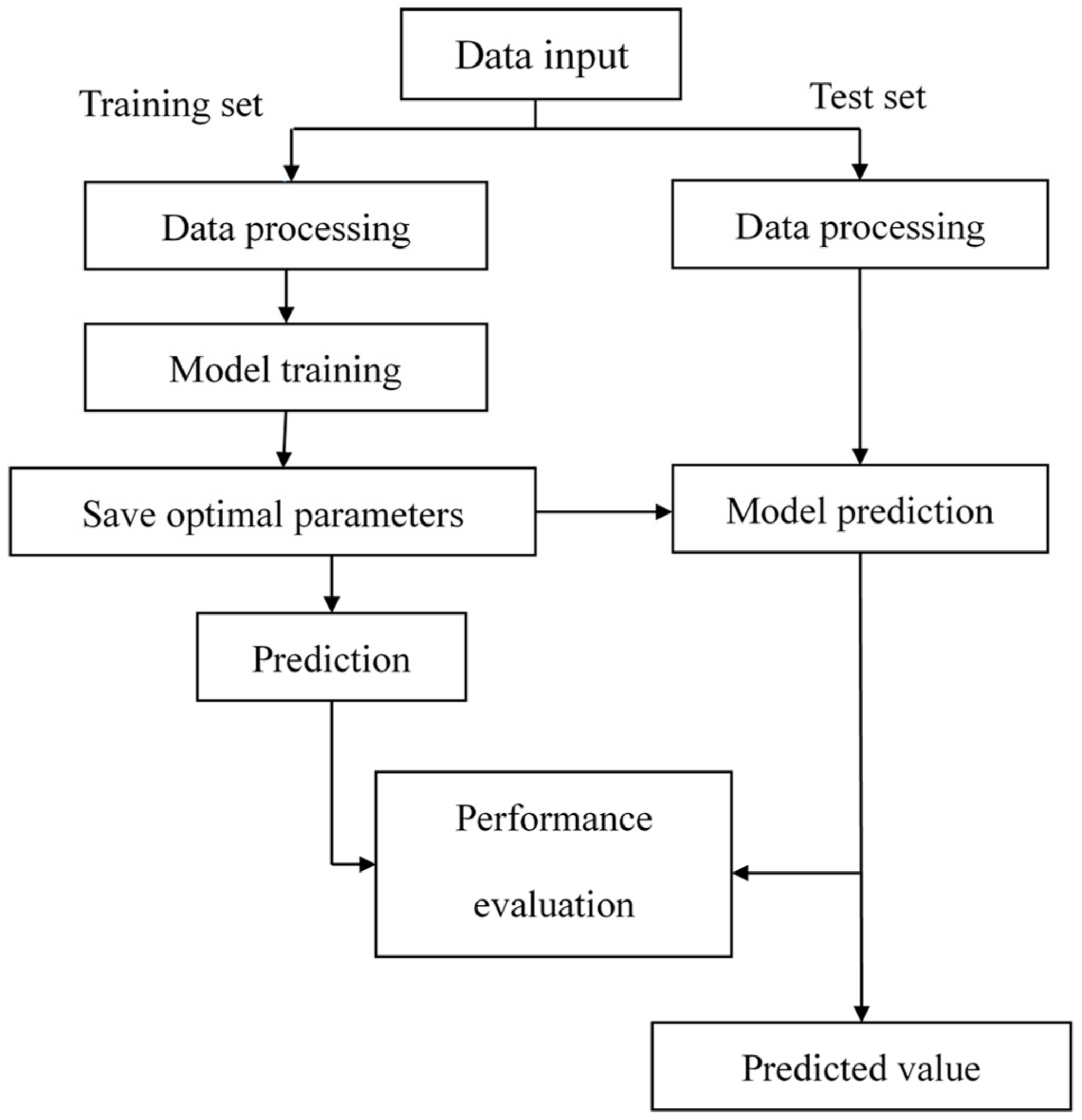
(5) Data output. In the permeability coefficient prediction task, the output is a continuous value that represents the predicted result of the permeability coefficient. Since the permeability coefficient of the input dataset is a value that has already been processed in the data preprocessing, the output can be directly used for the estimation of the permeability coefficient. In the subsequent prediction process, we only need to input the relevant parameters to obtain the predicted value of the permeability coefficient.

The CNN prediction model flowchart is shown in Figure 2.

3. Data Acquisition and Processing

There are some factors that affect the permeability coefficient significantly, including the gradation, pore ratio, coefficient of uniformity, and coefficient of curvature. For rockfill material, the size and distribution of particles may directly affect the velocity of the permeability of water. Gradation reflects the particle distribution of the rockfill material. The coefficient of uniformity measures the degree of dispersion in the particle size of the rockfill material. The highly inhomogeneous stones create larger penetration paths, which affect permeability. The coefficient of curvature characterizes the shapes of the particles. The pore ratio reflects the volume of pores in the soil, which relates to the water-flow area of the rockfill material and also affects permeability.

Some scholars, through experimental research, put forward their own empirical formulae to predict the coefficient of permeability of soil, such as Hazen’s formula, $K=d_{10}^2$, and Sauerbrey’s [26] formula, $K_{18}=\frac{c{n}^3{d}_{17}^2}{{(1-n)}^2}$, as well as Terzaghi’s formula and Kozeny’s formula, mentioned above, through which it can be concluded that the coefficient of permeability is a function of the parameters of the particle gradation, porosity, pore ratio, and so on, and it is possible to estimate the coefficient of permeability from these parameters. It can be concluded that the above parameters have a greater influence on the permeability coefficient and play a major controlling role in the prediction of the permeability coefficient. At the same time, the above parameters are easy to measure and obtain, which satisfies the purpose of the non-destructive and rapid measurement of the permeability coefficients of heap stone materials proposed in this paper.

Therefore, the neural network CNN model mainly learns the dataset, refines and analyzes the features between each datum and establishes a fitting relationship, so as to achieve the purpose of prediction. In this paper, by using the full feature particle size, Cc, Cu, and e as the input parameters and the permeability coefficient as the output parameter, a fitting relationship is established for the prediction of the permeability coefficient of heap rock material.

3.1. Data Acquisition and Processing

The determination process of the permeability coefficient of rockfill material samples using laboratory tests is cumbersome and the data format is difficult to unify. The data on the permeability coefficients of rockfill material and coarse-grained soil samples were obtained from the literature, scientific journals, academic papers, or research reports in relevant fields. The permeability coefficients of the samples were selected to be in the range of 10⁻³~10⁻¹ cm/s to ensure the applicability of the dataset to the rockfill materials due to the large permeability coefficients of rockfill materials. The particle-size range of the selected samples was between 5 mm and 60 mm, which is a typical range for large particle sizes. The permeability characteristics of the selected samples were similar to those of the rockfill material, which met the requirements of model training.

The original data for the dataset were provided by Ding et al. [27]. Based on the original data, the samples with permeability coefficients on the order of 10⁻⁴ cm/s were removed. The coefficient of uniformity C_u and the coefficient of curvature C_c were added to the dataset. The gradation, the pore ratio, the C_u, and the C_c were taken as the input features of the model and the permeability coefficients were taken as the output features. The collated dataset is shown in

Table 1. Sample data sets.

Sample	Characteristic Particle Size/mm										e	Cu	Cc	K20/ (cm·s−1)
	d10	d20	d30	d40	d50	d60	d70	d80	d90	d100
1	1.30	6.04	7.49	8.90	11.52	16.34	23.19	33.52	46.13	60.00	0.27	12.57	2.64	0.050
2	1.45	6.06	7.57	9.19	12.36	17.86	25.52	36.01	47.84	60.00	0.27	12.32	2.21	0.050
3	2.10	6.15	7.84	9.88	13.86	19.91	28.42	39.86	49.65	60.00	0.27	9.48	1.47	0.040
4	2.94	6.18	8.12	10.80	15.15	21.37	30.88	41.80	50.84	60.00	0.27	7.27	1.05	0.030
5	3.14	6.29	8.52	11.60	15.98	22.68	33.96	44.62	52.06	60.00	0.27	7.22	1.02	0.021
6	3.30	6.37	8.88	12.46	17.47	25.69	37.56	46.51	52.99	60.00	0.27	7.78	0.93	0.021
7	3.46	6.48	9.48	13.45	18.76	28.76	40.57	48.19	53.95	60.00	0.27	8.31	0.90	0.020
8	3.46	6.56	9.88	14.03	19.91	32.19	43.05	49.65	54.27	60.00	0.27	9.30	0.88	0.010
9	2.36	6.52	9.15	12.83	17.68	24.65	34.36	44.09	51.75	60.00	0.28	10.44	1.44	0.011
10	2.36	6.52	9.15	12.83	17.68	24.65	34.36	44.09	51.75	60.00	0.27	10.44	1.44	0.010
11	2.36	6.52	9.15	12.83	17.68	24.65	34.36	44.09	51.75	60.00	0.24	10.44	1.44	0.008
12	2.36	6.52	9.15	12.83	17.68	24.65	34.36	44.09	51.75	60.00	0.22	10.44	1.44	0.007
13	0.25	0.50	1.00	1.61	2.54	4.06	6.03	8.38	12.42	20.00	0.35	16.24	0.99	0.008
14	0.25	0.50	1.00	1.61	2.54	4.06	6.03	8.38	12.42	20.00	0.37	16.24	0.99	0.022
15	0.25	0.50	1.00	1.61	2.54	4.06	6.03	8.38	12.42	20.00	0.44	16.24	0.99	0.033
16	0.25	0.50	1.00	1.61	2.54	4.06	6.03	8.38	12.42	20.00	0.46	16.24	0.99	0.038
17	0.25	0.50	1.00	1.61	2.54	4.06	6.03	8.38	12.42	20.00	0.51	16.24	0.99	0.072
18	0.25	0.50	1.00	1.61	2.54	4.06	6.03	8.38	12.42	20.00	0.53	16.24	0.99	0.087
19	0.25	0.50	1.00	1.61	2.54	4.06	6.03	8.38	12.42	20.00	0.56	16.24	0.99	0.094
20	0.25	0.94	2.32	4.69	7.70	10.45	12.73	14.95	17.26	20.00	0.45	41.80	2.06	0.067
21	0.25	0.87	2.11	4.04	6.44	9.05	11.57	14.09	16.75	20.00	0.45	36.20	1.97	0.045
22	0.25	0.75	1.69	2.74	3.94	5.89	9.22	12.42	15.87	20.00	0.45	23.56	1.94	0.024
23	0.25	0.72	1.48	2.40	3.28	4.42	6.29	9.44	13.84	20.00	0.45	17.68	1.98	0.023
24	0.25	0.69	1.31	2.13	2.77	3.44	4.42	7.26	13.11	20.00	0.45	13.76	2.00	0.021
25	0.25	0.73	1.09	1.41	1.79	2.49	3.67	5.92	11.43	20.00	0.45	9.96	1.91	0.019
26	0.25	0.63	0.91	1.15	1.36	1.60	2.11	4.02	10.32	20.00	0.45	6.40	2.07	0.010
27	0.25	0.56	0.66	0.74	0.83	0.97	1.25	1.94	7.21	20.00	0.45	3.88	1.80	0.010
28	0.25	0.53	0.61	0.67	0.71	0.77	0.84	0.97	1.78	20.00	0.45	3.08	1.93	0.009
29	0.25	0.32	0.38	0.45	0.76	5.00	6.71	7.94	10.00	20.00	0.39	20.00	0.12	0.003
30	0.25	0.38	0.57	1.03	2.52	5.00	6.56	7.84	10.00	20.00	0.39	20.00	0.26	0.006
31	0.25	0.38	0.78	1.67	3.05	5.00	6.48	7.80	10.00	20.00	0.39	20.00	0.49	0.006
32	0.25	0.39	0.97	2.11	3.44	5.00	6.40	7.75	10.00	20.00	0.39	20.00	0.75	0.007
33	0.25	0.42	1.16	2.29	3.54	5.00	6.40	7.70	10.00	20.00	0.39	20.00	1.08	0.007
34	0.25	0.46	1.37	2.39	3.59	5.00	6.36	7.70	10.00	20.00	0.39	20.00	1.50	0.013
35	0.25	0.54	1.56	2.57	3.69	5.00	6.32	7.66	10.00	20.00	0.39	20.00	1.95	0.012
36	0.25	0.94	1.98	2.86	3.83	5.00	6.29	7.66	10.00	20.00	0.39	20.00	3.14	0.016
37	0.25	1.28	2.24	3.03	3.92	5.00	6.25	7.61	10.00	20.00	0.39	20.00	4.01	0.016
38	0.25	1.63	2.45	3.18	3.99	5.00	6.21	7.61	10.00	20.00	0.39	20.00	4.80	0.024
39	0.25	0.33	0.40	0.50	0.71	1.00	1.25	1.51	2.00	5.00	0.55	4.00	0.64	0.022
40	0.25	0.37	0.50	0.71	1.00	1.42	2.00	2.73	3.70	5.00	0.55	5.68	0.70	0.055
41	0.25	0.39	0.56	0.82	1.28	2.00	2.61	3.27	4.03	5.00	0.55	8.00	0.63	0.056
42	0.25	0.40	0.63	1.00	2.00	2.53	3.07	3.60	4.23	5.00	0.55	10.12	0.63	0.060
43	0.25	0.36	0.50	0.79	1.29	2.00	2.61	3.27	4.03	5.00	0.71	8.00	0.50	0.014
44	0.25	0.43	0.68	1.00	1.46	2.00	2.57	3.23	4.02	5.00	0.71	8.00	0.92	0.020
45	0.25	0.50	1.00	1.32	1.63	2.00	2.52	3.17	3.99	5.00	0.71	8.00	2.00	0.034
46	0.25	0.78	1.15	1.41	1.67	2.00	2.50	3.14	3.97	5.00	0.71	8.00	2.65	0.041
47	0.25	1.00	1.26	1.47	1.69	2.00	2.48	3.12	3.96	5.00	0.71	8.00	3.18	0.055
48	0.82	2.66	5.91	10.28	13.23	16.55	19.97	23.55	27.60	31.50	0.22	20.18	2.57	0.794
49	0.60	2.26	5.32	9.81	12.85	16.26	19.74	23.41	27.43	31.50	0.20	27.10	2.90	0.789
50	0.17	1.26	3.81	8.12	11.98	15.42	19.17	22.86	27.27	31.50	0.09	90.71	5.54	0.070
51	5.00	7.36	9.50	12.99	17.84	26.00	35.84	45.05	52.46	60.00	0.27	5.20	0.69	0.354
52	5.00	7.36	9.50	12.99	17.84	26.00	35.84	45.05	52.46	60.00	0.22	5.20	0.69	0.290
53	2.40	5.00	7.50	10.22	15.58	22.00	30.41	39.59	49.48	60.00	0.27	9.17	1.07	0.101
54	2.40	5.00	7.50	10.22	15.58	22.00	30.41	39.59	49.48	60.00	0.25	9.17	1.07	0.090
55	1.00	2.13	5.00	7.58	11.03	16.00	24.91	32.63	43.23	60.00	0.27	16.00	1.56	0.010
56	1.00	2.13	5.00	7.58	11.03	16.00	24.91	32.63	43.23	60.00	0.22	16.00	1.56	0.008
57	0.48	1.08	2.00	5.00	7.94	12.00	17.12	25.06	37.34	60.00	0.27	25.00	0.69	0.008
58	0.48	1.08	2.00	5.00	7.94	12.00	17.12	25.06	37.34	60.00	0.25	25.00	0.69	0.004
59	0.48	1.08	2.00	5.00	7.94	12.00	17.12	25.06	37.34	60.00	0.22	25.00	0.69	0.005
60	0.20	1.51	2.50	3.71	5.00	6.50	6.96	8.03	10.00	40.00	0.44	32.50	4.81	0.016
61	0.20	1.22	2.30	3.56	5.00	6.70	7.55	9.42	14.24	40.00	0.44	33.50	3.95	0.023
62	0.20	0.87	2.00	3.41	5.00	6.90	7.88	10.33	17.56	40.00	0.44	34.50	2.90	0.037
63	0.20	0.51	1.80	3.21	5.00	7.10	8.33	11.85	21.11	40.00	0.44	35.50	2.28	0.046
64	0.20	0.41	1.40	2.94	5.00	7.30	8.99	14.21	24.48	40.00	0.44	36.50	1.34	0.059
65	0.20	0.36	1.00	2.64	5.00	7.50	10.00	17.20	26.93	40.00	0.44	37.50	0.67	0.080
66	0.20	0.34	0.60	2.23	5.00	7.60	11.63	20.00	28.79	40.00	0.44	38.00	0.24	0.100
67	0.20	0.32	0.50	1.74	5.00	8.20	14.04	22.34	30.18	40.00	0.44	41.00	0.15	0.121
68	0.20	0.30	0.43	1.14	5.00	9.50	16.89	24.31	31.32	40.00	0.44	47.50	0.10	0.202
69	0.20	0.30	0.40	0.75	5.00	11.50	19.27	25.90	32.16	40.00	0.44	57.50	0.07	0.266
70	0.20	0.29	0.38	0.56	5.00	15.50	21.19	26.87	32.84	40.00	0.44	77.50	0.05	0.291
71	2.50	6.50	12.78	20.86	25.07	30.14	36.54	43.53	50.52	60.00	0.26	12.06	2.17	0.950
72	2.50	5.70	9.32	13.83	19.97	25.07	31.76	40.59	49.21	60.00	0.26	10.03	1.39	0.730
73	0.60	1.60	3.18	5.47	7.89	10.92	14.70	21.05	31.48	50.00	0.26	18.20	1.54	0.066
74	0.10	0.35	0.95	1.87	3.67	6.70	12.22	21.43	29.30	40.00	0.33	67.00	1.35	0.007
75	0.10	0.35	0.95	1.87	3.67	6.70	12.22	21.43	29.30	40.00	0.24	67.00	1.35	0.001
76	0.18	0.80	1.55	2.44	3.97	6.75	12.32	21.60	29.30	40.00	0.32	37.50	1.98	0.012
C1	0.25	0.70	1.77	2.71	3.76	5.00	6.32	7.70	10.00	20.00	0.39	20.00	2.51	0.010
C2	0.25	0.80	1.95	3.32	5.10	7.43	10.14	12.96	16.16	20.00	0.45	29.72	2.05	0.028
C3	2.36	6.52	9.15	12.83	17.68	24.65	34.36	44.09	51.75	60.00	0.25	10.44	1.44	0.009
C4	0.25	0.50	1.00	1.61	2.54	4.06	6.03	8.38	12.42	20.00	0.41	16.24	0.99	0.023
C5	5.00	7.36	9.50	12.99	17.84	26.00	35.84	45.05	52.46	60.00	0.25	5.20	0.69	0.305
C6	1.00	2.13	5.00	7.58	11.03	16.00	24.91	32.63	43.23	60.00	0.25	16.00	1.56	0.009

.

3.2. Model Performance Evaluation

In this paper, the root mean square error (RMSE), coefficient of determination (R²), and mean absolute error (MAE) are used as the evaluation indexes to assess the performance of the model. The RMSE is an index to assess the difference between predicted values and test values. A smaller RMSE indicates that the difference between the predictions and the observations is smaller, meaning a better model performance. Its expression is as follows:

$$RMSE=\sqrt{\frac{1}{m}{\displaystyle \sum _{i=1}^m{(y_i-\widehat{y_i})}^2}}$$

(7)

R² is used to measure how well the model explains the total variance. It represents the proportion of the total variance explained by the model and takes a value between 0 and 1. A larger R² indicates that the model explains the variability of the test data better and that the model fit is better. Its expression is as follows:

$$R^2=1-\frac{{\displaystyle \sum _i{(\widehat{y_i}-y_i)}^2}}{{\displaystyle \sum _i{({\overline{y}}_i-y_i)}^2}}$$

(8)

The MAE is the average of the absolute errors between the predicted and the test values. A smaller MAE value indicates a smaller absolute error in the model prediction, meaning better model performance. Its expression is:

$$MAE=\frac{1}{m}{\displaystyle \sum _{i=1}^m|(}{y}_i-\widehat{y_i})|$$

(9)

where $y_i$ and $\widehat{y_i}$ are the test and predicted values of the permeability coefficient, respectively, m is the total number of samples, and $\overline{y_i}$ is the mean of the test values.

4. Model Training and Results Analysis

Building the BP neural network model and the random forest model and comparing them with the CNN model allows us to assess the performance of the CNN model with respect to the BP model in the permeability coefficient prediction task. This comparison helps us to understand the advantages of the CNN model.

4.1. Construction of the BP Model

The full name of the BP neural network is the backpropagation neural network, which is a multilayer feed-forward network trained according to the error-backpropagation algorithm. The BP neural network model is a classical neural network model that has been widely used in a variety of prediction and classification tasks. It has a multilayer structure and a backpropagation algorithm to model and learn complex nonlinear relationships. It consists of input, hidden, and output layers. The construction of the BP neural network can be achieved by the self-contained toolbox in MATLAB-R2022a [28]. The specific construction steps are as follows:

(1) Data normalization and sample division.

(2) Define input, hidden, and output layers. The number of hidden layers is determined by the empirical formula $J=\sqrt{m+n}+a$ (where $J$ is the number of neurons in the hidden layer, m is the number of neurons in the input layer, n is the number of neurons in the output layer, and a is a constant between 0 and 10).

(3) Define the network training function and parameter settings. The activation function is a sigmoid function, the number of iterations is set to 1000, the learning rate is 0.01, and the error threshold is 1 × 10⁻⁶.

(4) Training model and performance evaluation.

The BP model’s hyperparameter settings are shown in

Table 2. BP model hyperparameters.

Parameters	Value
Number of iterations	1000
Error threshold	1 × 10−6
Learning rate	0.01

.

4.2. Analysis of Training Results

The collected dataset was used in the model training. During the training process, the hyperparameters needed to be adjusted according to the training effect to improve the prediction accuracy. Furthermore, to verify the prediction performance of the model, the CNN model was compared to the traditional BP model and the error of each model was calculated. The training effect is shown in Figure 3 and Figure 4, and the evaluation index of each model is shown in

Table 3. Model-evaluation indexes.

Index	Training Set		Testing Set
	CNN	BP	CNN	BP
RMSE	0.043	0.125	0.147	0.364
R2	0.902	0.742	0.808	0.659
MAE	0.027	0.042	0.105	0.148

.

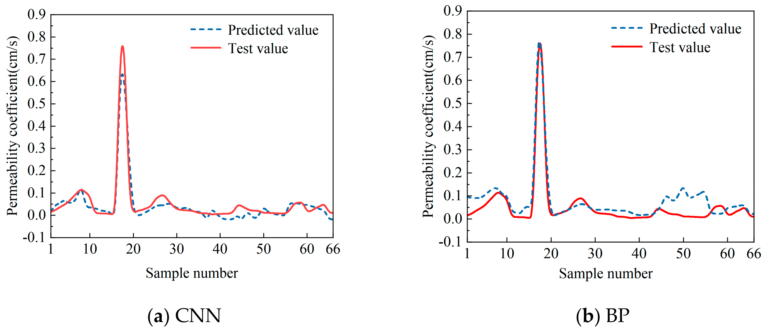
As can be seen in Figure 3, the CNN model and the BP model both perform well on the training set. However, the predicted values of the BP model fluctuate greatly, and the predicted values of some samples deviate from the test values significantly. On the other hand, the predicted values of the CNN model are closer to the test values, and the trends are also consistent with the test values. Therefore, the CNN model fits the dataset better.

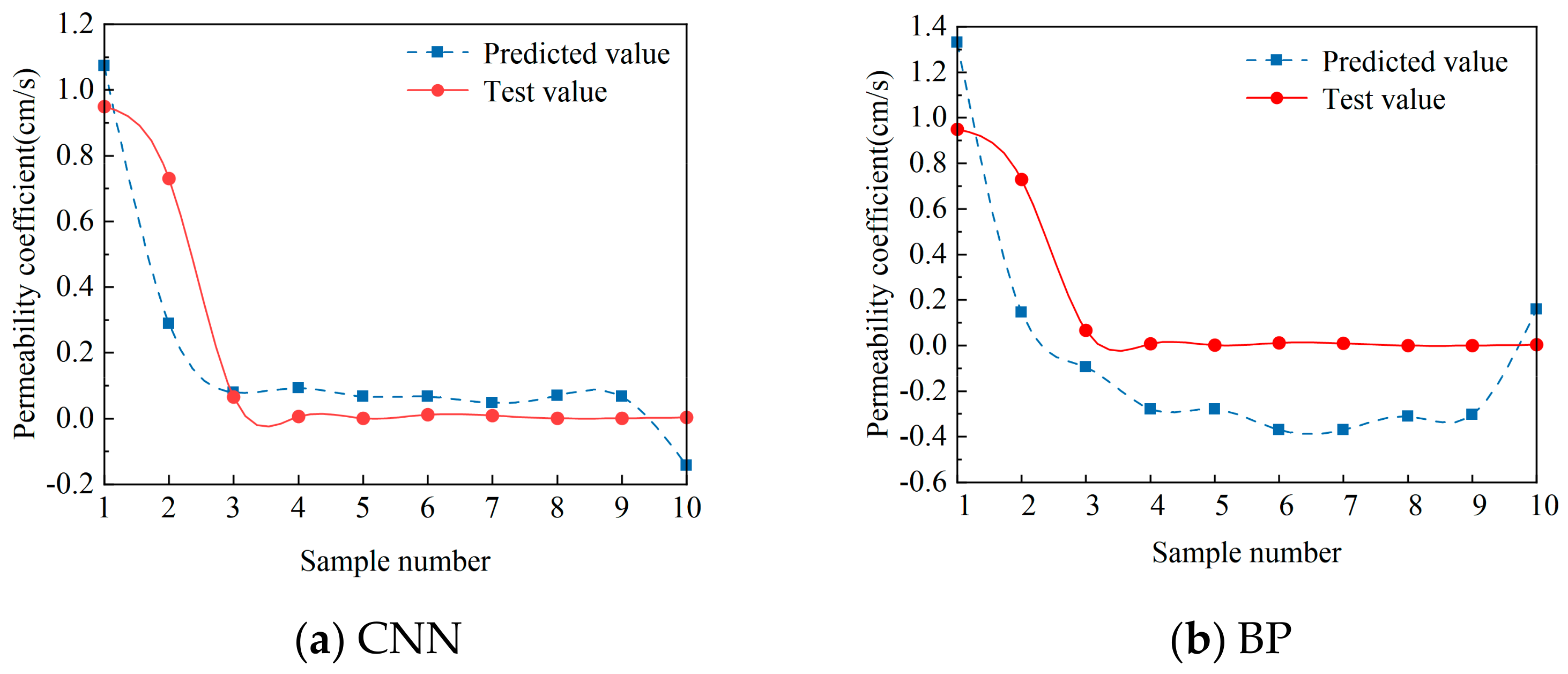
As can be seen in Figure 4, the predicted values of the CNN model are closer to the test values than those of the BP model, with less fluctuation in the curve and a more stable trend, indicating that the CNN model has higher prediction accuracy and better model performance. In addition, the CNN model has a better prediction effect when the test value of the sample permeability coefficient is about 0.1 cm/s or less, but the prediction accuracy is lower when the permeability coefficient is larger. The main reason for this is the small number of datasets (76 groups). The permeability coefficients of the dataset samples are concentrated around the order of 1 × 10⁻² cm/s. The number of samples above 0.1 cm/s is small, providing insufficient data for the CNN model. Even on the dataset with only 76 sets of samples, the CNN model has good results, showing the powerful learning and fitting ability of the CNN, which also performs well in regression problems.

In Table 3, the evaluation indexes of the CNN model and BP model are compared and analyzed. For RMSE, the CNN model’s training set decreases by 65.6% and the testing set decreases by 59.62% compared with the BP model. For R², the CNN model improves the training set by 21.56% and the testing set by 22.61% compared with the BP model. For MAE, the CNN model decreases the training set by 35.71% and the testing set by 29.05% compared with the BP model. Thus, it seems that the convolutional and pooling layers in the CNN model contribute to improving the ability to extract the feature information of the data, which significantly improves the prediction performance and verifies the model’s applicability in the prediction of the permeability coefficients of rockfill materials.

The model’s prediction accuracy was tested using non-participating training data. The comparison of the predicted values and test values is shown in

Table 4. Comparison of predicted and test values of the CNN model.

Number	Test Value/(cm·s−1)	Predicted Value/(cm·s−1)	Relative Error/%
C1	1.00 × 10−2	1.07 × 10−2	7.00
C2	2.80 × 10−2	2.85 × 10−2	1.78
C3	9.00 × 10−3	8.83 × 10−3	1.89
C4	2.30 × 10−2	2.12 × 10−2	7.83
C5	3.05 × 10−1	3.23 × 10−1	5.90
C6	9.00 × 10−3	9.38 × 10−3	4.22

. It can be seen that the maximum relative error between the CNN model’s predicted values and the test values is 7.83% and that the average relative error is 4.77%, indicating that the predicted values are closer to the test values.

4.3. Model Effectiveness Evaluation

To validate the performance of the CNN model and the BP model, the mainstream machine learning evaluation method of K-fold cross-validation is used. The steps of K-fold cross-validation are as follows: first, the original dataset is divided into K subsets of similar size, and next, K iterations are performed. In each iteration, one of the subsets is used as the test set and the remaining K-1 subsets are used as the training set. Next, the training set is used to train the model and the performance of the model is evaluated on the corresponding test set. The performance-evaluation results obtained from K iterations are averaged as the final performance-evaluation results.

In this study, the dataset was divided into seven subsets, one subset was used as the test set each time, and the results of the seven subsets were obtained as shown in

Table 5. MAE values for each subset of the CNN model and BP model.

Number	Training Set		Testing Set
	CNN	BP	CNN	BP
1	0.035	0.069	0.098	0.216
2	0.027	0.023	0.173	0.252
3	0.035	0.063	0.093	0.137
4	0.028	0.048	0.095	0.190
5	0.033	0.018	0.102	0.183
6	0.032	0.031	0.026	0.053
7	0.024	0.027	0.159	0.277
average	0.031	0.039	0.106	0.187

, which shows that the CNN model performs well on each validation subset and that the model is sufficiently reliable.

5. Validation of Permeability Test

To validate the generalization performance of the CNN model, a constant head permeability test was conducted to verify the prediction accuracy of the model [29]. In the normal head infiltration test, since the infiltration head remains stable, the pore structure of the soil body is more uniform after it is compacted by equal compaction work, and no turbulence occurs during the test; the soil body can be described as having laminar flow, and its infiltration coefficient can be calculated by applying Darcy’s formula.

5.1. Permeability Test Design

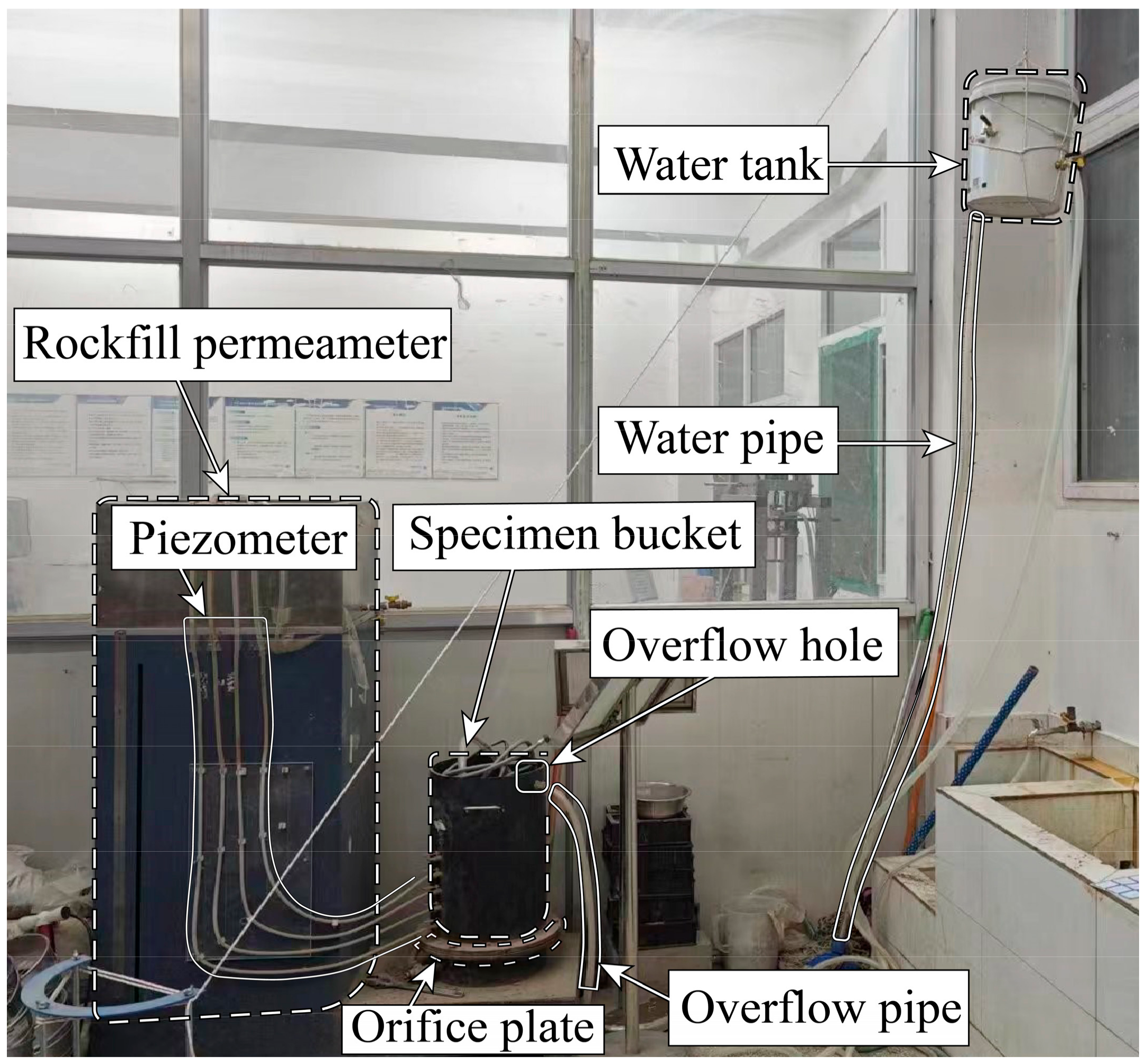
The permeameter sample gradation adopted the reduced scale of the field gradation of the rockfill dam. The samples were formulated to ensure good gradation, which is controlled by the coefficient of uniformity and the coefficient of curvature. Furthermore, the large particles greater than 60 mm in size were excluded, and the particle-size range was 2–60 mm. The rockfill permeameter was used in the test as shown in Figure 5. The diameter of the specimen bucket was 300 mm. The test was conducted with a water temperature of 20 °C as the standard temperature, and the permeability coefficient was measured at this standard temperature.

The specific steps of the permeability test are as follows:

(1) Instrument installation. The water pipe was connected and the water was filled from the bottom of the instrument until the water level was slightly above the orifice plate and the water supply was stopped. Samples were taken and the air-dried water contents of the samples were measured. The temperature (T) during the test was recorded.

(2) The samples were filled into the specimen buckets in layers and lightly tamped with a wooden hammer. After filling, the height from the top of the specimen to the top of the bucket was measured and the net height of the specimen was calculated. The mass of the filled samples was calculated by measuring the mass of the remaining samples. A buffer layer of gravel approximately 2 cm thick was placed over the top of the specimen. The water supply was slightly opened until the water level rose to the overflow hole, and then the water supply was stopped.

(3) After a few minutes, the water level in each piezometer was checked to ensure that it was flush with the overflow hole. The water supply was started to allow water to be injected into the specimen bucket. During the test, the water supply should be adjusted to allow the supply water slightly more than the overflow water. The overflow pipe should always have water overflow to maintain a constant water level.

(4) After the water level of the piezometer tube has been stabilized, the water level of the piezometer tube should be recorded and the difference in water level between each piezometer tube should be calculated. The volume of infiltration water in a certain period (t) was taken with a graduated cylinder, and the measurement should be repeated according to the regulations.

The permeability coefficient of the constant head permeability test should be calculated according to the following formula:

$$K_{\mathrm{T}}=\frac{2QL}{At\left(H_1+H_2\right)}$$

(10)

$$K_{20}=K_{\mathrm{T}}\frac{{\eta }_{ \mathrm{T}}}{{\eta }_{ 20}}$$

(11)

where K_T is the permeability coefficient of the specimen at the target water temperature (T) (cm/s), Q is the volume of infiltration water in a certain period (t), in seconds (cm³), L is the seepage diameter (cm), the height between the centers of the two pressure holes, A is the cross-sectional area of the specimen (cm²), t is the time (s), H₁, H₂ is the difference between the water levels (cm), K₂₀ is the permeability coefficient of the specimen at the standard water temperature (20 °C) (cm/s), ${\eta }_{\mathrm{T}}$ is the coefficient of the dynamic viscosity of the water at the target water temperature (T) (1 × 10⁻⁶ kPa·s), and ${\eta }_{20}$ is the coefficient of the dynamic viscosity of water under the standard water temperature (20 °C) (1 × 10⁻⁶ kPa·s).

5.2. Permeability Test Results

The permeability test results of the samples are shown in

Table 6. Test results of samples.

Sample	Characteristic Particle Size/mm										e	Cu	Cc	K20 (cm/s)
	d10	d20	d30	d40	d50	d60	d70	d80	d90	d100
1	0.39	1.34	3.52	7.19	11.63	17.36	24.25	32.13	40.04	60.00	0.540	44.30	1.82	0.1349
2	0.30	1.02	2.32	4.20	7.12	11.32	17.31	26.31	37.76	60.00	0.452	37.80	1.59	0.0933
3	0.24	0.44	1.31	2.82	4.98	8.93	14.17	19.89	33.90	60.00	0.184	37.83	0.81	0.0812

.

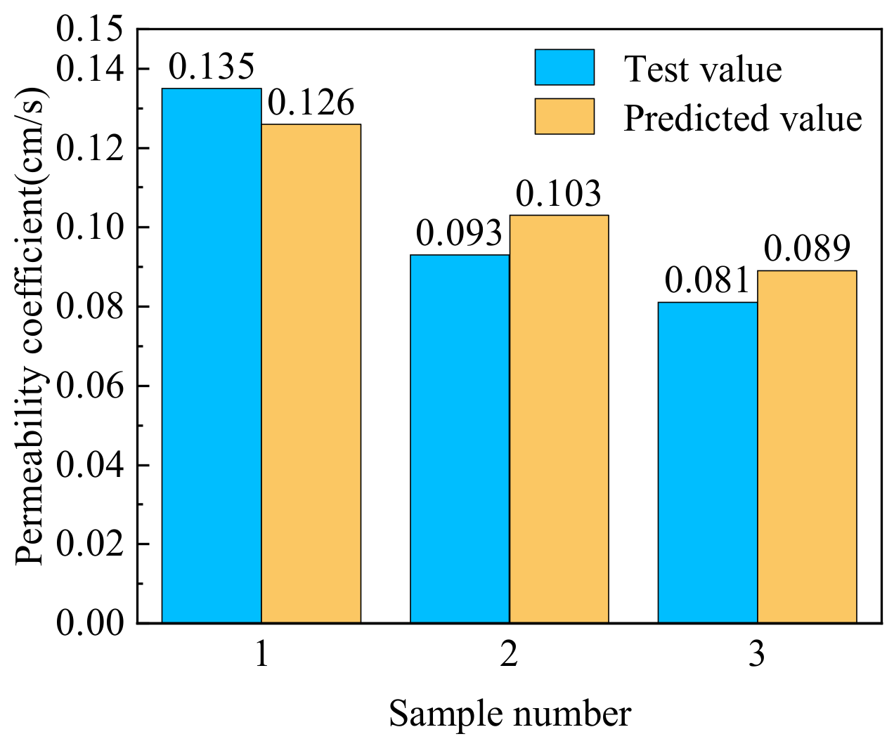
The comparison of the test values and the predicted values is shown in

Table 7. Predicted values and relative errors of the samples.

Sample	Permeability Coefficient (cm/s)
	Test Value	Predicted Value	Relative Error
1	0.135	0.126	6.67%
2	0.093	0.103	10.75%
3	0.081	0.089	9.87%

and Figure 6. The complexity of the infiltration path of the rockfill material is related to many factors, such as the compactness, gradation, pore ratio, coefficient of uniformity, etc. Therefore, some error exists between the predicted permeability coefficient obtained with the CNN model and the test values. From Table 7 and Figure 6, it can be seen that the difference between the predicted values of the CNN model and the test values of the permeability test is not large and that the relative error is small, which meets the general needs of rough estimation in engineering. Therefore, the CNN model is applicable when evaluate the permeability coefficient of rockfill material.

6. Conclusions

With the popularization of machine learning technology, the application of neural networks in engineering practice has received increasing attention. In this paper, the CNN was used to establish a machine learning model to predict the permeability coefficient of rockfill material, and the following conclusions were obtained:

(1) Compared with the traditional BP neural network, CNNs can learn to obtain more data features through their special convolution and pooling structures. Therefore, they have higher accuracy in regression prediction.

(2) For the prediction of the permeability coefficient of rockfill material, the gradation, coefficient of uniformity, coefficient of curvature, and pore ratio were used as the input features and the permeability coefficient was used as the output feature to build a dataset, which achieved better results.

(3) The laboratory permeability test was conducted to demonstrate that the CNN model has good generalization performance.

References

- Eggleston, J.; Rojstaczer, S. The value of grain-size hydraulic conductivity estimates: Comparison with high resolution in-situ field hydraulic conductivity. Geophys. Res. Lett. 2001, 28, 4255–4258. [Google Scholar] [CrossRef]
- Zhu, C.H.; Liu, J.M.; Wang, Z.H. Study on the influence of particle level matching on permeability coefficient of coarse-grained soil. People’s Yellow River 2005, 12, 79–81. (In Chinese) [Google Scholar]
- Chapuis, R.P. Predicting the saturated hydraulic conductivity of soils: A review. Bull. Eng. Geol. Environ. 2012, 71, 401–434. [Google Scholar] [CrossRef]
- Zhou, W.H.; Yuen, K.V.; Tan, F. Estimation of soil–water characteristic curve and relative permeability for granular soils with different initial dry densities. Eng. Geol. 2014, 179, 1–9. [Google Scholar] [CrossRef]
- Göktepe, A.B.; Sezer, A. Effect of particle shape on density and permeability of sands. Proc. Inst. Civ. Eng. Geotech. Eng. 2010, 163, 307–320. [Google Scholar] [CrossRef]
- Ghabchi, R.; Zaman, M.; Kazmee, H.; Singh, D. Effect of shape parameters and gradation on laboratory-measured permeability of aggregate bases. Int. J. Geomech. 2015, 15, 04014070. [Google Scholar] [CrossRef]
- Seghir, A.; Benamar, A.; Wang, H. Effects of fine particles on the suffusion of cohesionless soils. Exp. Model. Transp. Porous Media 2014, 103, 233–247. [Google Scholar] [CrossRef]
- Sato, M.; Kuwano, R. Suffusion and clogging by one-dimensional seepage tests on cohesive soil. Soils Found. 2015, 55, 1427–1440. [Google Scholar] [CrossRef]
- Tillmann, A.; Englert, A.; Nyari, Z.; Fejes, I.; Vanderborght, J.; Vereecken, H. Characterization of subsoil heterogeneity, estimation of grain size distribution and hydraulic conductivity at the Krauthausen test site using cone penetration test. J. Contam. Hydrol. 2008, 95, 57–75. [Google Scholar] [CrossRef]
- Wang, J.J.; Qiu, Z.F. Anisotropic hydraulic conductivity and critical hydraulic gradient of a crushed sandstone–mudstone particle mixture. Mar. Georesour. Geotechnol. 2017, 35, 89–97. [Google Scholar] [CrossRef]
- Neithalath, N.; Sumanasooriya, M.S.; Deo, O. Characterizing pore volume, sizes, and connectivity in pervious concretes for permeability prediction. Mater. Charact. 2010, 61, 802–813. [Google Scholar] [CrossRef]
- Koohmishi, M.; Azarhoosh, A. Assessment of permeability of granular drainage layer considering particle size and air void distribution. Constr. Build. Mater. 2021, 270, 121373. [Google Scholar] [CrossRef]
- Chapuis, R.P. Predicting the saturated hydraulic conductivity of sand and gravel using effective diameter and void ratio. Can. Geotech. J. 2004, 41, 787–795. [Google Scholar] [CrossRef]
- Koohmishi, M. Hydraulic conductivity and water level in the reservoir layer of porous pavement considering gradation of aggregate and compaction level. Constr. Build. Mater. 2019, 203, 27–44. [Google Scholar] [CrossRef]
- Dolzyk, K.; Chmielewska, I. Predicting the coefficient of permeability of non-plastic soils. Soil Mech. Found. Eng. 2014, 51, 213–218. [Google Scholar] [CrossRef]
- Wrzesiński, G.; Markiewicz, A. Prediction of permeability coefficient k in sandy soils using ANN. Sustainability 2022, 14, 6736. [Google Scholar] [CrossRef]
- Pham, B.T.; Ly, H.B.; Al-Ansari, N.; Ho, L.S. A comparison of Gaussian process and M5P for prediction of soil permeability coefficient. Sci. Program. 2021, 2021, 3625289. [Google Scholar] [CrossRef]
- Tran, V.Q. Predicting and investigating the permeability coefficient of soil with aided single machine learning algorithm. Complexity 2022, 2022, 8089428. [Google Scholar] [CrossRef]
- Ahmad, M.; Keawsawasvong, S.; Bin Ibrahim, M.R.; Waseem, M.; Kashyzadeh, K.R.; Sabri, M.M.S. Novel approach to predicting soil permeability coefficient using Gaussian process regression. Sustainability 2022, 14, 8781. [Google Scholar] [CrossRef]
- Yilmaz, I.; Marschalko, M.; Bednarik, M.; Kaynar, O.; Fojtova, L. Neural computing models for prediction of permeability coefficient of coarse-grained soils. Neural Comput. Appl. 2012, 21, 957–968. [Google Scholar] [CrossRef]
- Zhang, R.; Zhang, S. Coefficient of permeability prediction of soils using gene expression programming. Eng. Appl. Artif. Intell. 2024, 128, 107504. [Google Scholar] [CrossRef]
- Al Khalifah, H.; Glover, P.W.J.; Lorinczi, P. Permeability prediction and diagenesis in tight carbonates using machine learning techniques. Mar. Pet. Geol. 2020, 112, 104096. [Google Scholar] [CrossRef]
- Dongare, A.D.; Kharde, R.R.; Kachare, A.D. Introduction to artificial neural network. Int. J. Eng. Innov. Technol. IJEIT 2012, 2, 189–194. [Google Scholar]
- Li, Z.; Liu, F.; Yang, W.; Peng, S.; Zhou, J. A Survey of Convolutional Neural Networks: Analysis, Applications, and Prospects. IEEE Trans. Neural Netw. Learn. Syst. 2022, 33, 6999–7019. [Google Scholar] [CrossRef] [PubMed]
- Vedaldi, A.; Lenc, K. Matconvnet: Convolutional neural networks for MATLAB. In Proceedings of the 23rd ACM International Conference on Multimedia, ACM, New York, NY, USA, 29 October–3 November 2015; pp. 689–692. [Google Scholar]
- Sauerbrey, I.I. On the problem and determination of the permeability coefficient. Proc. VNIIG 1932, 3–5, 115–145. (In Russian) [Google Scholar]
- Ding, Y.; Rao, Y.K.; Ni, Q.; Xu, W.N.; Liu, D.X.; Zhang, H. Effect of particle composition and pore ratio on permeability coefficient of coarse-grained soil. Hydrogeol. Eng. Geol. 2019, 46, 108–116. (In Chinese) [Google Scholar]
- Liu, L.; Chen, J.; Xu, L. Realization and application research of BP neural network based on MATLAB. In Proceedings of the 2008 International Seminar on Future BioMedical Information Engineering, Wuhan, China, 18 December 2008; pp. 130–133. [Google Scholar]
- Sandoval, G.F.; Galobardes, I.; Teixeira, R.S.; Toralles, B.M. Comparison between the falling head and the constant head permeability tests to assess the permeability coefficient of sustainable pervious concretes. Case Stud. Constr. Mater. 2017, 7, 317–328. [Google Scholar] [CrossRef]