
Evaluation Method of Severe Convective Precipitation Based on Dual-Polarization Radar Data

 ,
,
Abstract
:1. Introduction
2. Dataset and Experimental Design
2.1. NJU-CPOL Dataset
2.2. Experimental Design
2.3. Evaluating Indicator
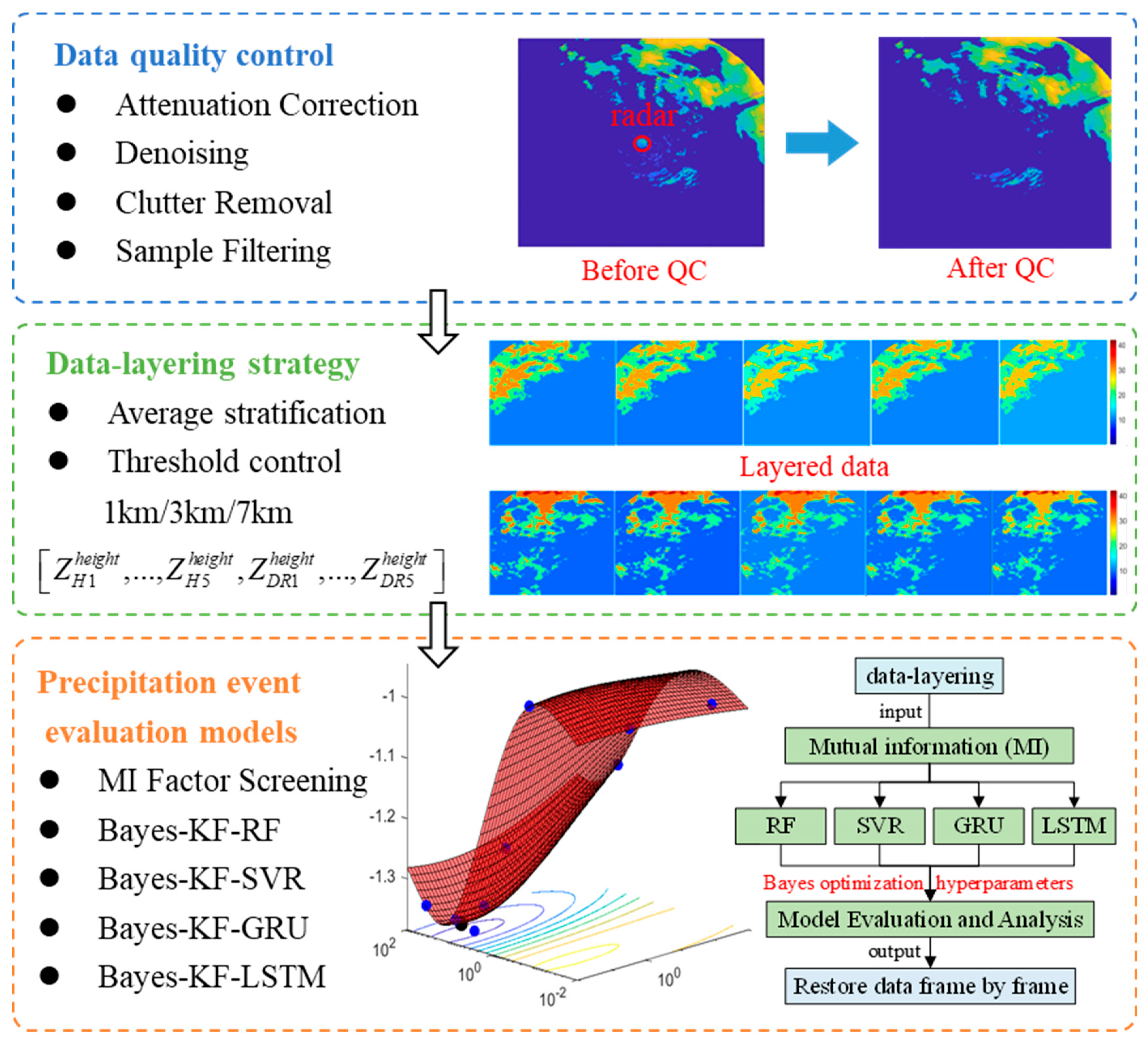
3. Methodology
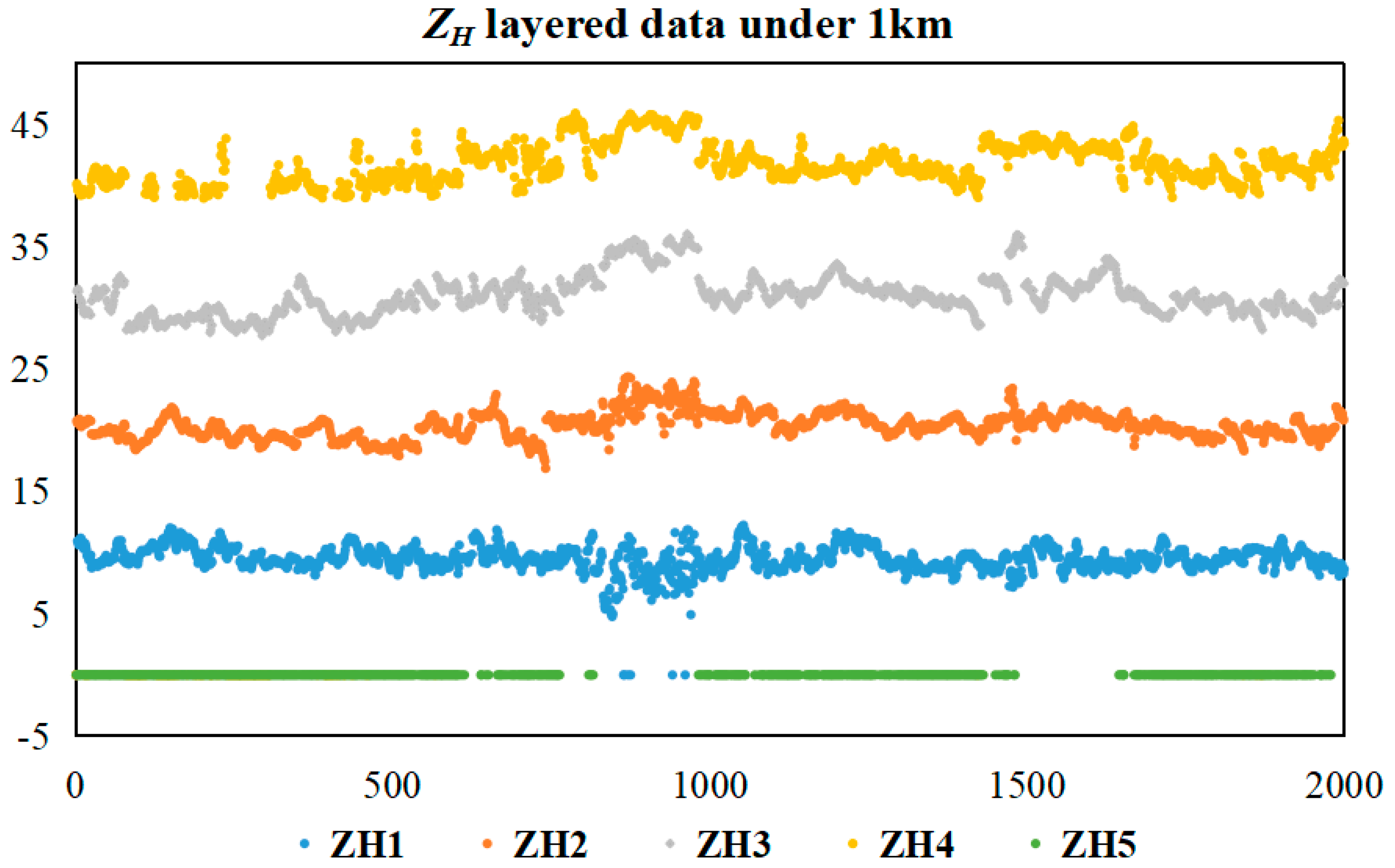
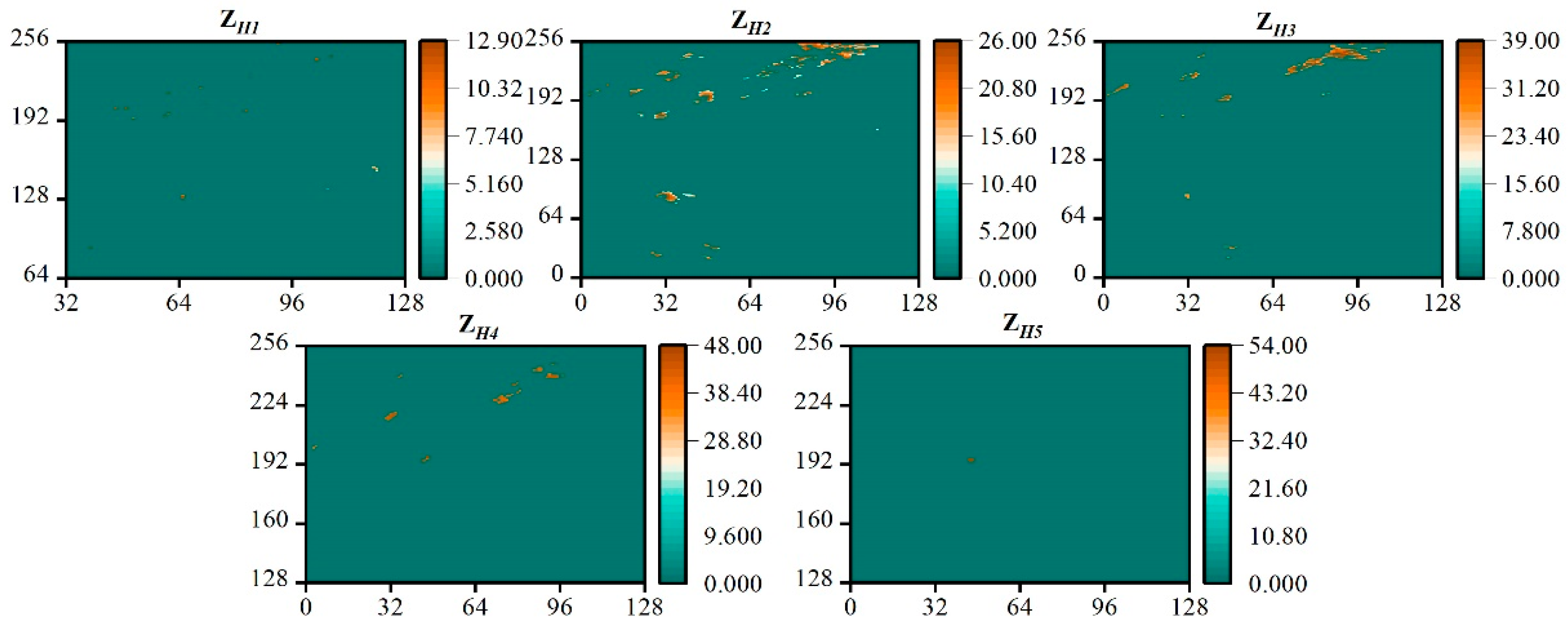
3.1. Data-Layering Strategy
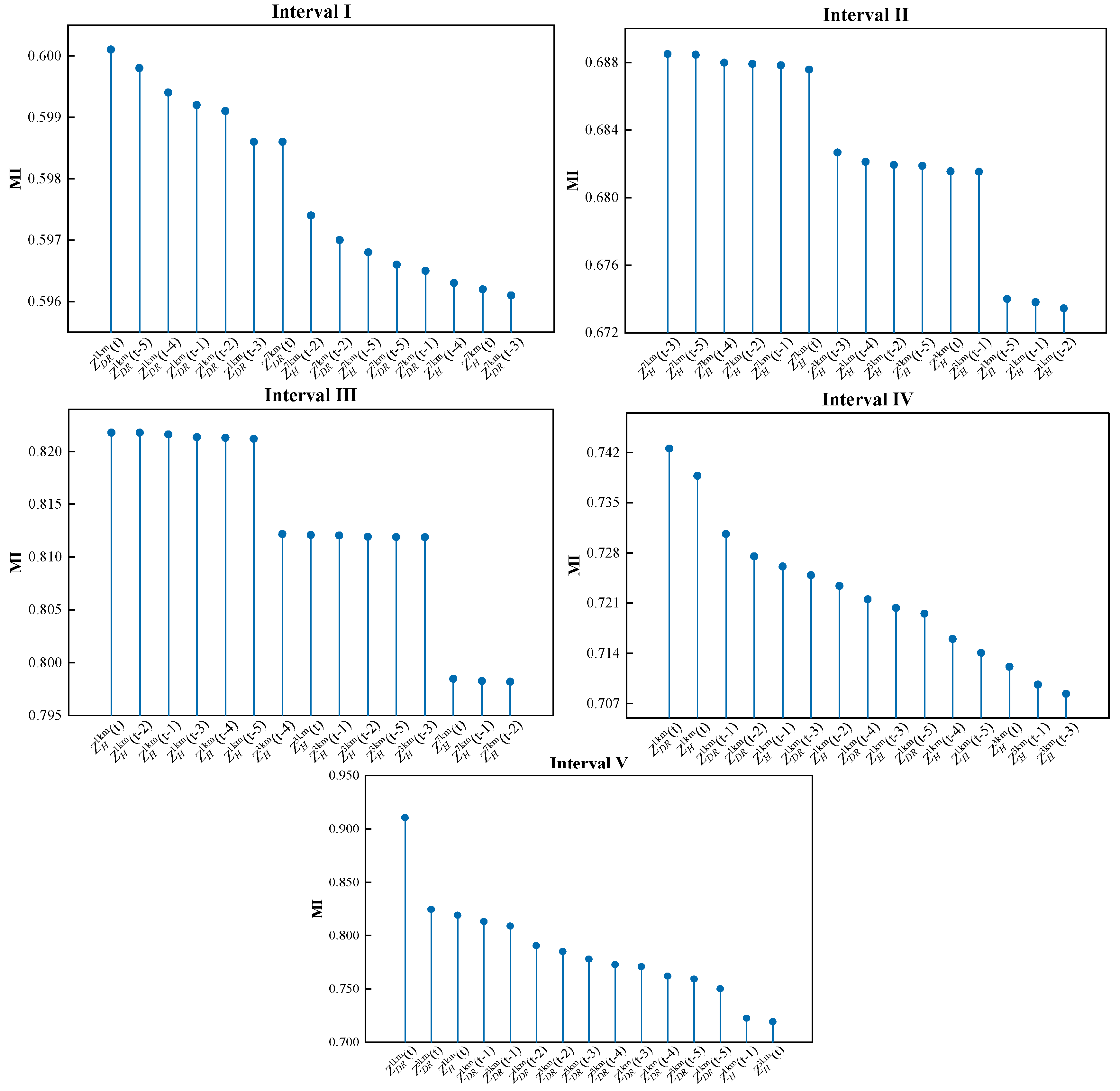
3.2. Factor Screening Method
3.3. Data Noise Reduction Method
3.4. Rainfall Assessment Model
3.4.1. Random Forest
3.4.2. Support Vector Regression
3.4.3. Gate Recurrent Unit
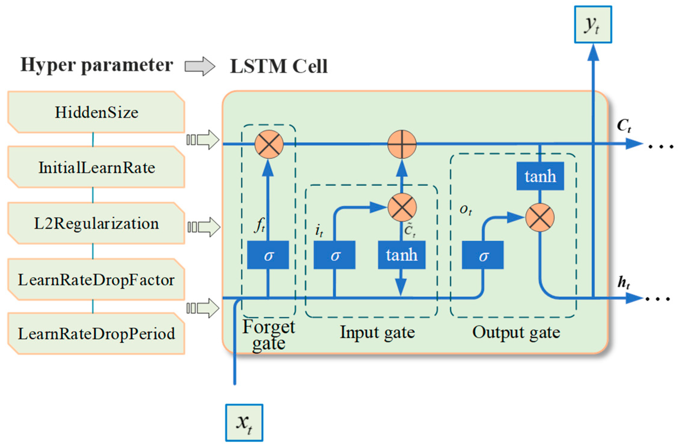
3.4.4. Long Short-Term Memory
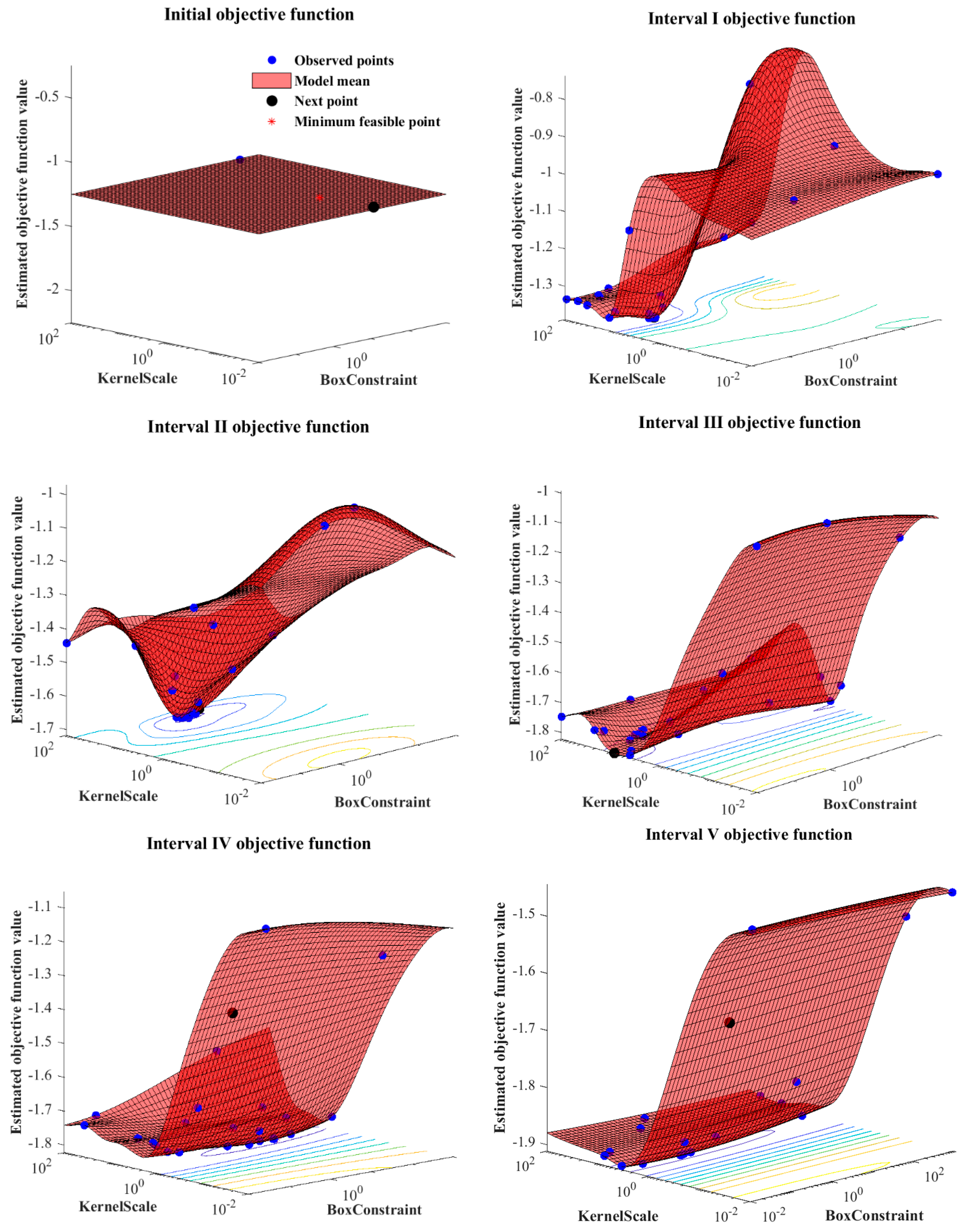
3.4.5. Bayesian Hyperparameter Optimization
4. Results Analysis
4.1. Data Stratification Results
4.2. Analysis of MI Results
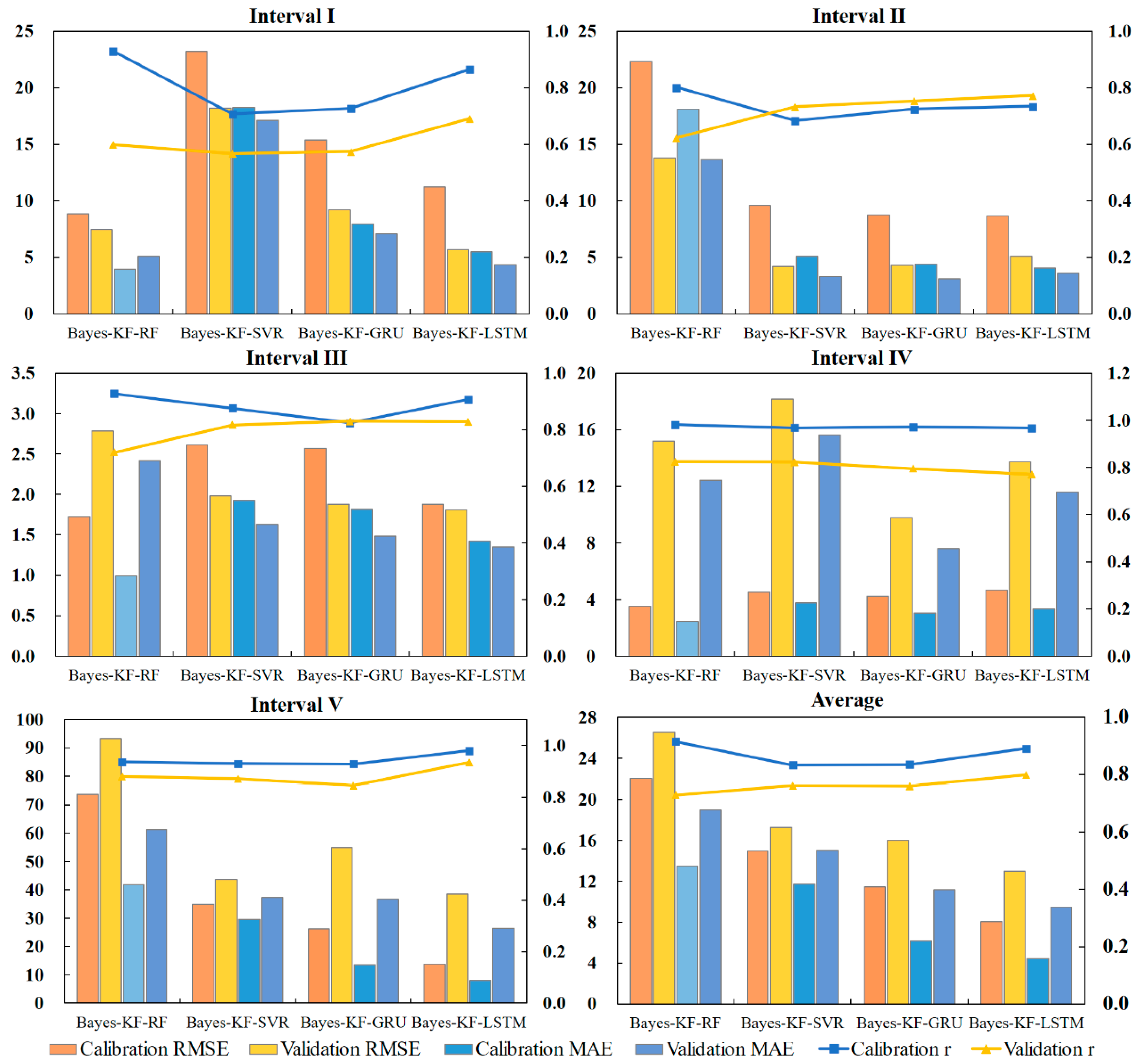
4.3. Interval Evaluation Effect
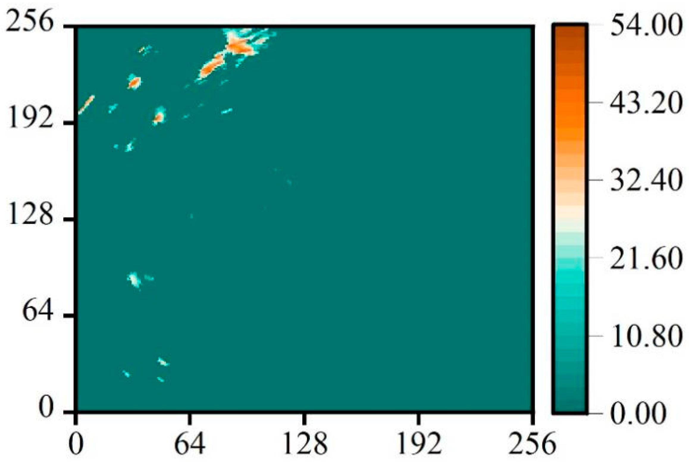
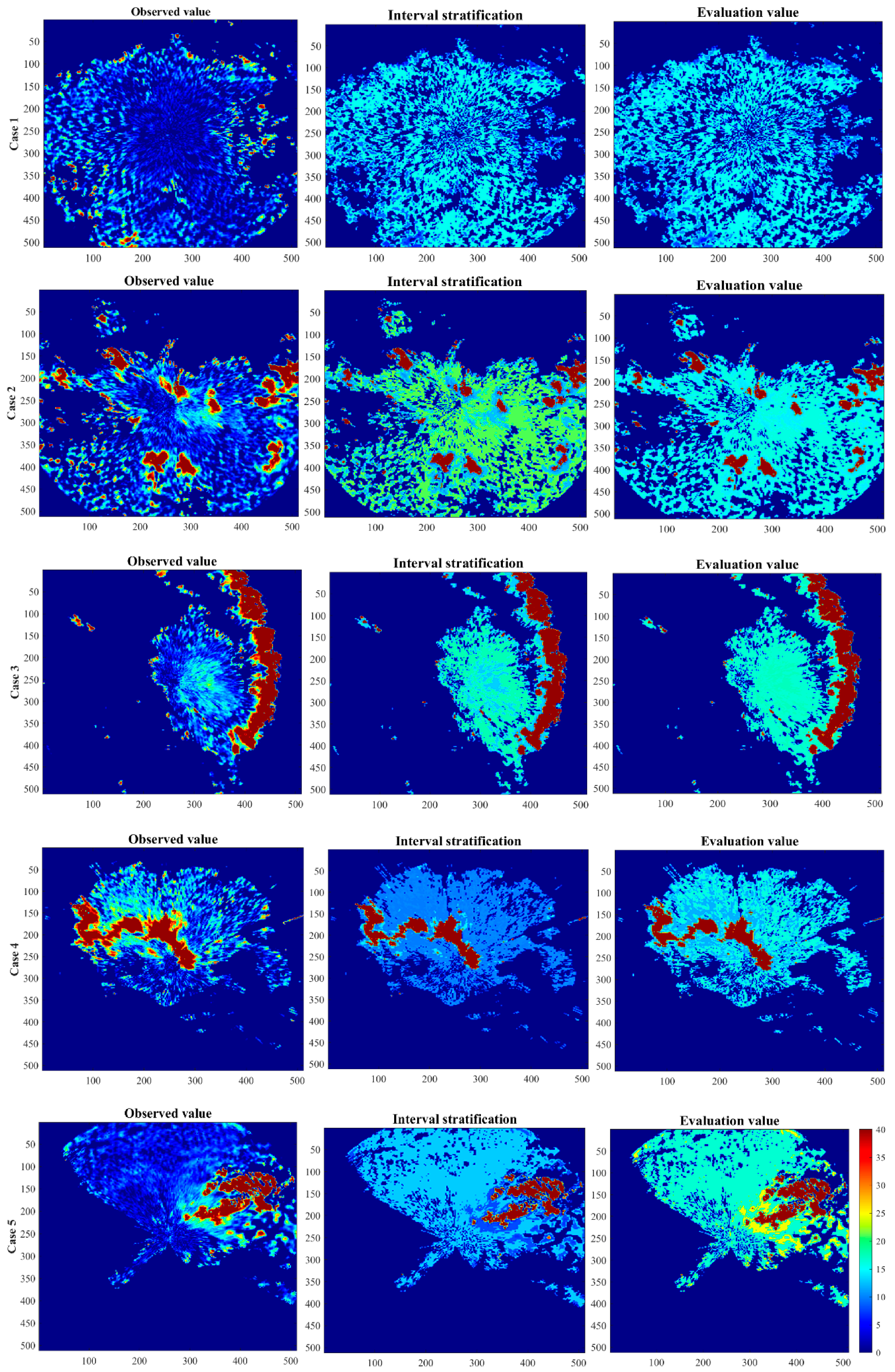
4.4. Representative Cases
5. Summary and Discussion
Author Contributions
Funding
Data Availability Statement
Conflicts of Interest
References
- Ma, Y.; Hu, Z.; Li, C.; Feng, T.; Meng, X.; Dong, W. Anthropogenic Climate Change Enhances the July 2021 Super-Heavy Rainfall Event in Central China. Bull. Am. Meteorol. Soc. 2023, 104, E736–E741. [Google Scholar] [CrossRef]
- Ma, Y.; Hu, Z.; Meng, X.; Liu, F.; Dong, W. Was the record-breaking mei-yu of 2020 enhanced by regional climate change. Bull. Amer. Meteor. Soc. 2022, 103, S76–S82. [Google Scholar] [CrossRef]
- Nashwan, M.S.; Shahid, S. Future precipitation changes in Egypt under the 1.5 and 2.0 C global warming goals using CMIP6 multimodel ensemble. Atmos. Res. 2022, 265, 105908. [Google Scholar] [CrossRef]
- Wang, X.; Li, Y.; Wang, M.; Li, Y.; Gong, X.; Chen, Y.; Chen, Y.; Cao, W. Changes in daily extreme temperature and precipitation events in mainland China from 1960 to 2016 under global warming. Int. J. Climatol. 2021, 41, 1465–1483. [Google Scholar] [CrossRef]
- Guo, J.; Feng, T.; Cai, Z.; Lian, X.; Tang, W. Vulnerability Assessment for power transmission lines under typhoon weather based on a cascading failure state transition diagram. Energies 2020, 13, 3681. [Google Scholar] [CrossRef]
- Wang, L.; Dong, Y.; Zhang, C.; Heng, Z. Extreme and severe convective weather disasters: A dual-polarization radar nowcasting method based on physical constraints and a deep neural network model. Atmos. Res. 2023, 289, 106750. [Google Scholar] [CrossRef]
- Cao, X.; Qi, Y.; Ni, G. X-band polarimetric radar QPE for urban hydrology: The increased contribution of high-resolution rainfall capturing. J. Hydrol. 2023, 617, 128905. [Google Scholar] [CrossRef]
- Chao, L.; Zhang, K.; Yang, Z.; Wang, J.; Lin, P.; Liang, J.; Li, Z.; Gu, Z. Improving flood simulation capability of the WRF-Hydro-RAPID model using a multi-source precipitation merging method. J. Hydrol. 2021, 592, 125814. [Google Scholar] [CrossRef]
- Wang, S.; Zhang, K.; Chao, L.; Li, D.; Tian, X.; Bao, H.; Chen, G.; Xia, Y. Exploring the utility of radar and satellite-sensed precipitation and their dynamic bias correction for integrated prediction of flood and landslide hazards. J. Hydrol. 2021, 603, 126964. [Google Scholar] [CrossRef]
- Senocak, A.U.G.; Yilmaz, M.T.; Kalkan, S.; Yucel, I.; Amjad, M. An explainable two-stage machine learning approach for precipitation forecast. J. Hydrol. 2023, 627, 130375. [Google Scholar] [CrossRef]
- Nikhil Teja, K.; Manikanta, V.; Das, J.; Umamahesh, N.V. Enhancing the predictability of flood forecasts by combining Numerical Weather Prediction ensembles with multiple hydrological models. J. Hydrol. 2023, 625, 130176. [Google Scholar] [CrossRef]
- Saminathan, S.; Medina, H.; Mitra, S.; Tian, D. Improving short to medium range GEFS precipitation forecast in India. J. Hydrol. 2021, 598, 126431. [Google Scholar] [CrossRef]
- Stevens, B.; Bony, S. What are climate models missing? Science 2013, 340, 1053–1054. [Google Scholar] [CrossRef] [PubMed]
- Ding, J.; Gao, J.; Zhang, G.; Zhang, F.; Yang, J.; Wang, S.; Xue, B.; Wang, K. A Rolling Real-Time Correction Method for Minute Precipitation Forecast Based on Weather Radars. Water 2023, 15, 1872. [Google Scholar] [CrossRef]
- Tian, W.; Wang, C.L.; Shen, K.L.; Zhang, L.X.; Sian, K. MSLKNet: A Multi-Scale Large Kernel Convolutional Network for Radar Extrapolation. Atmosphere 2024, 15, 52. [Google Scholar] [CrossRef]
- Capecchi, V.; Antonini, A.; Benedetti, R.; Fibbi, L.; Melani, S.; Rovai, L.; Ricchi, A.; Cerrai, D. Assimilating X-and S-band Radar Data for a Heavy Precipitation Event in Italy. Water 2021, 13, 1727. [Google Scholar] [CrossRef]
- Ansh Srivastava, N.; Mascaro, G. Improving the utility of weather radar for the spatial frequency analysis of extreme precipitation. J. Hydrol. 2023, 624, 129902. [Google Scholar] [CrossRef]
- Shi, E.; Li, Q.; Gu, D.; Zhao, Z. A Method of Weather Radar Echo Extrapolation Based on Convolutional Neural Networks. In Proceedings of the 24th International Conference, MMM 2018, Bangkok, Thailand, 5–7 February 2018. [Google Scholar] [CrossRef]
- Song, C.M. Data construction methodology for convolution neural network based daily runoff prediction and assessment of its applicability. J. Hydrol. 2022, 605, 127324. [Google Scholar] [CrossRef]
- Guo, J.; Liu, Y.; Zou, Q.; Ye, L.; Zhu, S.; Zhang, H. Study on optimization and combination strategy of multiple daily runoff prediction models coupled with physical mechanism and LSTM. J. Hydrol. 2023, 624, 129969. [Google Scholar] [CrossRef]
- Trebing, K.; Staǹczyk, T.; Mehrkanoon, S. SmaAt-UNet: Precipitation nowcasting using a small attention-UNet architecture. Pattern Recognit. Lett. 2021, 145, 178–186. [Google Scholar] [CrossRef]
- Yao, Y.; Li, Z. 2017CIKM AnalytiCup 2017: Short-term precipitation forecasting based on radar reflectivity images. In Proceedings of the Conference on Information and Knowledge Management, Short-Term Quantitative Precipitation Forecasting Challenge, Singapore, 6–10 November 2017. [Google Scholar]
- Yu, Z.; Ming, W.; Nan, L.I.; Ilyas, A.M. Improved radar heavy precipitation estimation based on RNN. China Sci. 2020, 15, 585–592. [Google Scholar]
- Guo, J.; Zhou, J.; Qin, H.; Zou, Q.; Li, Q. Monthly streamflow forecasting based on improved support vector machine model. Expert Syst. Appl. 2011, 38, 13073–13081. [Google Scholar] [CrossRef]
- Otsubo, A.; Adachi, A. Short-Term Predictability of Extreme Rainfall Using Dual-Polarization Radar Measurements. J. Meteorol. Soc. Jpn. 2024, 102, 151–165. [Google Scholar] [CrossRef]
- Xiao, M.Y.; Wang, L.; Dong, Y.C.; Zhang, C.H.; Wang, S.J.; Yang, K.Q.; Zhang, K. An early warning approach for the rapid identification of extreme weather disasters based on phased array dual polarization radar cooperative network data. PLoS ONE 2024, 19, e0296044. [Google Scholar] [CrossRef] [PubMed]
- Zhang, G.; Mahale, V.N.; Putnam, B.J.; Qi, Y.; Cao, Q.; Byrd, A.D.; Bukovcic, P.; Zrnic, D.S.; Gao, J.; Xue, M. Current status and future challenges of weather radar polarimetry: Bridging the gap between radar meteorology/hydrology/engineering and numerical weather prediction. Adv. Atmos. Sci. 2019, 36, 571–588. [Google Scholar] [CrossRef]
- Crisologo, I.; Vulpiani, G.; Abon, C.C.; David, C.; Bronstert, A.; Heistermann, M. Polarimetric rainfall retrieval from a C-Band weather radar in a tropical environment (The Philippines). Asia Pac. J. Atmos. Sci. 2014, 50, 595–607. [Google Scholar] [CrossRef]
- Pallardy, Q.; Fox, N.I. Accounting for rainfall evaporation using dual-polarization radar and mesoscale model data. J. Hydrol. 2018, 557, 573–588. [Google Scholar] [CrossRef]
- Zhao, K.; Huang, H.; Wang, M.; Lee, W.; Chen, G.; Wen, L.; Wen, J.; Zhang, G.; Xue, M.; Yang, Z. Recent progress in dual-polarization radar research and applications in China. Adv. Atmos. Sci. 2019, 36, 961–974. [Google Scholar] [CrossRef]
- Wang, M.; Zhao, K.; Xue, M.; Zhang, G.; Liu, S.; Wen, L.; Chen, G. Precipitation microphysics characteristics of a Typhoon Matmo (2014) rainband after landfall over eastern China based on polarimetric radar observations. J. Geophys. Res. Atmos. 2016, 121, 412–415,433. [Google Scholar] [CrossRef]
- Pan, X.; Lu, Y.; Zhao, K.; Huang, H.; Wang, M.; Chen, H. Improving Nowcasting of convective development by incorporating polarimetric radar variables into a deep-learning model. Geophys. Res. Lett. 2021, 48, e2021GL095302. [Google Scholar] [CrossRef]
- Wen, G.; Fox, N.I.; Market, P.S. The Quality Control and Rain Rate Estimation for the X-Band Dual-Polarization Radar: A Study of Propagation of Uncertainty. Remote Sens. 2020, 12, 1072. [Google Scholar] [CrossRef]
- Zhao, G.; Huang, H.; Yu, Y.; Zhao, K.; Yang, Z.W.; Chen, G.; Zhang, Y. Study on the Quantitative Precipitation Estimation of X-Band Dual-Polarization Phased Array Radar from Specific Differential Phase. Remote Sens. 2023, 15, 359. [Google Scholar] [CrossRef]
- Huang, H.; Zhao, K.; Zhang, G.; Lin, Q.; Wen, L.; Chen, G.; Yang, Z.; Wang, M.; Hu, D. Quantitative Precipitation Estimation with Operational Polarimetric Radar Measurements in Southern China: A Differential Phase–Based Variational Approach. J. Atmos. Ocean. Technol. 2018, 35, 1253–1271. [Google Scholar] [CrossRef]
- Cao, Y.; Zhang, D.; Zheng, X.; Shan, H.; Zhang, J. Mutual Information Boosted Precipitation Nowcasting from Radar Images. Remote Sens. 2023, 15, 1639. [Google Scholar] [CrossRef]
- Ning, Y.; Liang, G.; Ding, W.; Shi, X.; Fan, Y.; Chang, J.; Wang, Y.; He, B.; Zhou, H. A Mutual Information Theory-Based Approach for Assessing Uncertainties in Deterministic Multi-Category Precipitation Forecasts. Water Resour. Res. 2022, 58, e2022WR032631. [Google Scholar] [CrossRef]
- Na, W.; Yoo, C. Real-time bias correction of Beaslesan dual-pol radar rain rate using the dual Kalman filter. J. Korea Water Resour. Assoc. 2020, 53, 201–214. [Google Scholar]
- Grewal, M.S.; Andrews, A.P.; Bartone, C.G. Kalman Filtering; Wiley Telecom: Hoboken, NJ, USA, 2020. [Google Scholar]
- Chen, C.; Hu, B.; Li, Y. Easy-to-use spatial random-forest-based downscaling-calibration method for producing precipitation data with high resolution and high accuracy. Hydrol. Earth Syst. Sci. 2021, 25, 5667–5682. [Google Scholar] [CrossRef]
- Sekulić, A.; Kilibarda, M.; Heuvelink, G.B.; Nikolić, M.; Bajat, B. Random forest spatial interpolation. Remote Sens. 2020, 12, 1687. [Google Scholar] [CrossRef]
- Zhang, C.; Wang, H.; Zeng, J.; Ma, L.; Guan, L. Short-term dynamic radar quantitative precipitation estimation based on wavelet transform and support vector machine. J. Meteorol. Res. 2020, 34, 413–426. [Google Scholar] [CrossRef]
- Zhang, F.; O’Donnell, L.J. Support vector regression. In Machine Learning; Elsevier: Amsterdam, The Netherlands, 2020; pp. 123–140. [Google Scholar]
- Cho, M.; Kim, C.; Jung, K.; Jung, H. Water level prediction model applying a long short-term memory (lstm)–gated recurrent unit (gru) method for flood prediction. Water 2022, 14, 2221. [Google Scholar] [CrossRef]
- Landi, F.; Baraldi, L.; Cornia, M.; Cucchiara, R. Working memory connections for LSTM. Neural Netw. 2021, 144, 334–341. [Google Scholar] [CrossRef] [PubMed]
- Sherstinsky, A. Fundamentals of recurrent neural network (RNN) and long short-term memory (LSTM) network. Phys. D Nonlinear Phenom. 2020, 404, 132306. [Google Scholar] [CrossRef]
- Cho, H.; Kim, Y.; Lee, E.; Choi, D.; Lee, Y.; Rhee, W. Basic enhancement strategies when using Bayesian optimization for hyperparameter tuning of deep neural networks. IEEE Access 2020, 8, 52588–52608. [Google Scholar] [CrossRef]
- Lee, S.; Bae, J.H.; Hong, J.; Yang, D.; Panagos, P.; Borrelli, P.; Yang, J.E.; Kim, J.; Lim, K.J. Estimation of rainfall erosivity factor in Italy and Switzerland using Bayesian optimization based machine learning models. Catena 2022, 211, 105957. [Google Scholar] [CrossRef]


| Model | Hyperparameters to Be Optimized | Number of Hyperparameters |
|---|---|---|
| RF | numTrees; MaxNumSplits; MinLeafSize | 3 |
| SVR | BoxConstraint; KernelScale | 2 |
| GRU | hiddenSize; InitialLearnRate; LearnRateDropFactor; LearnRateDropPeriod | 4 |
| LSTM | hiddenSize; InitialLearnRate; L2Regularization; LearnRateDropFactor; LearnRateDropPeriod | 5 |
| Interval | Input Factors |
|---|---|
| Ⅰ | |
| Ⅱ | |
| Ⅲ | |
| Ⅳ | |
| Ⅴ |
| Data Range | Model | Period | r | RMSE | MAE |
|---|---|---|---|---|---|
| Interval Ⅰ | Bayes–KF-RF | Calibration | 0.93 | 8.83 | 3.96 |
| Validation | 0.60 | 7.48 | 5.08 | ||
| Bayes–KF-SVR | Calibration | 0.71 | 23.19 | 18.25 | |
| Validation | 0.57 | 18.18 | 17.14 | ||
| Bayes–KF-GRU | Calibration | 0.73 | 15.37 | 7.98 | |
| Validation | 0.57 | 9.21 | 7.05 | ||
| Bayes–KF-LSTM | Calibration | 0.87 | 11.23 | 5.46 | |
| Validation | 0.69 | 5.67 | 4.36 | ||
| Interval Ⅱ | Bayes–KF-RF | Calibration | 0.80 | 22.31 | 18.09 |
| Validation | 0.62 | 13.81 | 13.67 | ||
| Bayes–KF-SVR | Calibration | 0.68 | 9.61 | 5.09 | |
| Validation | 0.73 | 4.22 | 3.31 | ||
| Bayes–KF-GRU | Calibration | 0.73 | 8.78 | 4.38 | |
| Validation | 0.75 | 4.30 | 3.10 | ||
| Bayes–KF-LSTM | Calibration | 0.73 | 8.64 | 4.06 | |
| Validation | 0.77 | 5.09 | 3.59 | ||
| Interval Ⅲ | Bayes–KF-RF | Calibration | 0.93 | 1.72 | 0.99 |
| Validation | 0.72 | 2.78 | 2.42 | ||
| Bayes–KF-SVR | Calibration | 0.88 | 2.61 | 1.92 | |
| Validation | 0.82 | 1.98 | 1.63 | ||
| Bayes–KF-GRU | Calibration | 0.82 | 2.57 | 1.81 | |
| Validation | 0.83 | 1.88 | 1.48 | ||
| Bayes–KF-LSTM | Calibration | 0.91 | 1.88 | 1.42 | |
| Validation | 0.83 | 1.81 | 1.35 | ||
| Interval Ⅳ | Bayes–KF-RF | Calibration | 0.98 | 3.50 | 2.46 |
| Validation | 0.82 | 15.19 | 12.41 | ||
| Bayes–KF-SVR | Calibration | 0.97 | 4.49 | 3.75 | |
| Validation | 0.82 | 18.16 | 15.65 | ||
| Bayes–KF-GRU | Calibration | 0.97 | 4.24 | 3.04 | |
| Validation | 0.80 | 9.77 | 7.58 | ||
| Bayes–KF-LSTM | Calibration | 0.97 | 4.66 | 3.32 | |
| Validation | 0.77 | 13.75 | 11.62 | ||
| Interval Ⅴ | Bayes–KF-RF | Calibration | 0.94 | 73.73 | 41.77 |
| Validation | 0.88 | 93.38 | 61.19 | ||
| Bayes–KF-SVR | Calibration | 0.93 | 34.86 | 29.60 | |
| Validation | 0.87 | 43.65 | 37.26 | ||
| Bayes–KF-GRU | Calibration | 0.93 | 26.29 | 13.59 | |
| Validation | 0.84 | 54.86 | 36.69 | ||
| Bayes–KF-LSTM | Calibration | 0.98 | 13.76 | 7.91 | |
| Validation | 0.93 | 38.56 | 26.37 |
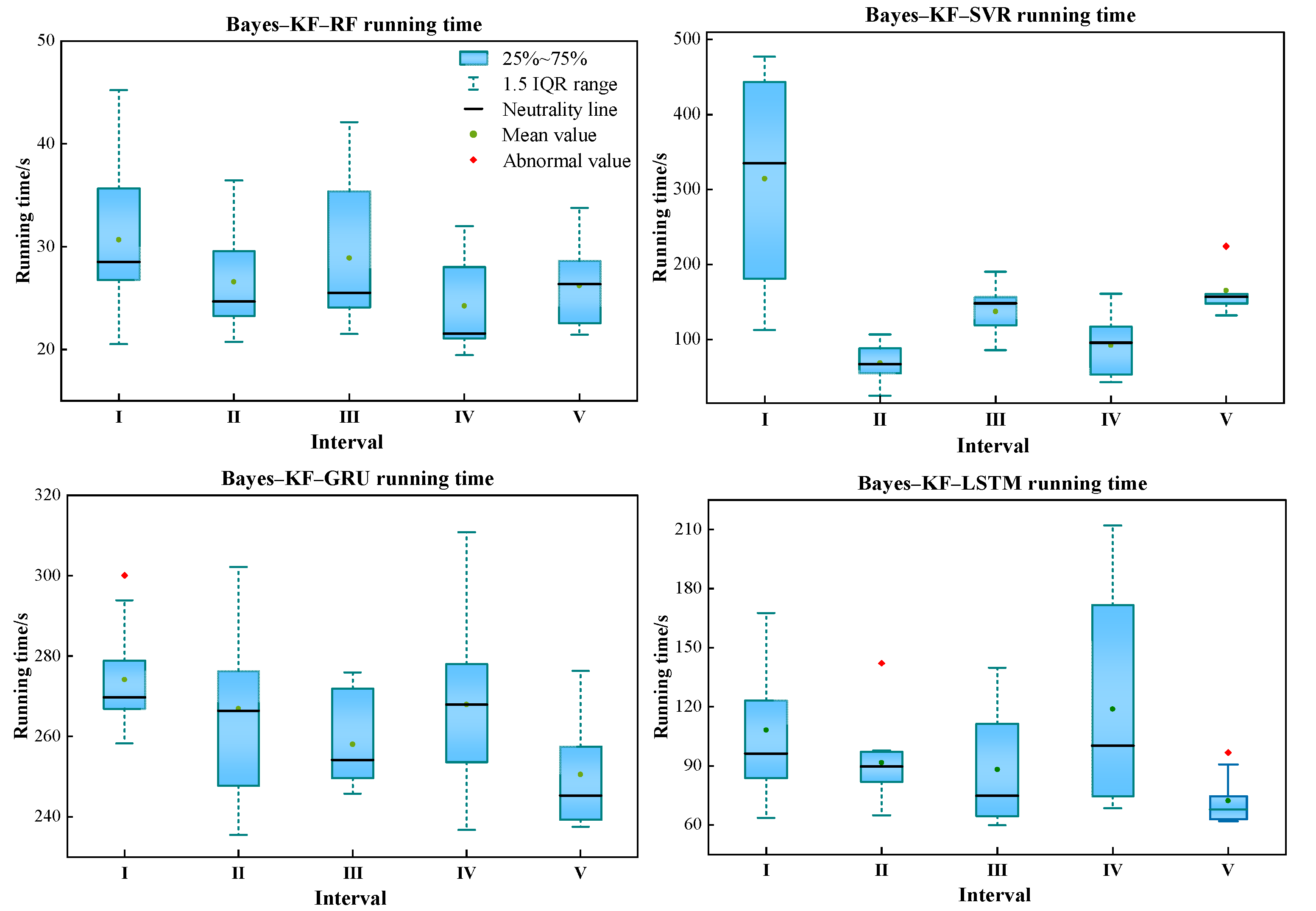
| Model | Interval | Running Time/s | Model | Interval | Running Time/s |
|---|---|---|---|---|---|
| Bayes–KF–RF | Ⅰ | 30.67 | Bayes–KF–GRU | Ⅰ | 274.13 |
| Ⅱ | 26.56 | Ⅱ | 266.89 | ||
| Ⅲ | 28.87 | Ⅲ | 258.02 | ||
| Ⅳ | 24.20 | Ⅳ | 267.91 | ||
| Ⅴ | 26.18 | Ⅴ | 250.48 | ||
| Bayes–KF–SVR | Ⅰ | 314.31 | Bayes–KF–LSTM | Ⅰ | 108.16 |
| Ⅱ | 68.69 | Ⅱ | 91.62 | ||
| Ⅲ | 137.20 | Ⅲ | 88.08 | ||
| Ⅳ | 92.42 | Ⅳ | 118.77 | ||
| Ⅴ | 165.28 | Ⅴ | 72.30 |
Disclaimer/Publisher’s Note: The statements, opinions and data contained in all publications are solely those of the individual author(s) and contributor(s) and not of MDPI and/or the editor(s). MDPI and/or the editor(s) disclaim responsibility for any injury to people or property resulting from any ideas, methods, instructions or products referred to in the content. |
© 2024 by the authors. Licensee MDPI, Basel, Switzerland. This article is an open access article distributed under the terms and conditions of the Creative Commons Attribution (CC BY) license (https://creativecommons.org/licenses/by/4.0/).
Share and Cite
Tang, Z.; Chang, X.; Ni, X.; Xiao, W.; Liu, H.; Guo, J. Evaluation Method of Severe Convective Precipitation Based on Dual-Polarization Radar Data. Water 2024, 16, 1136. https://doi.org/10.3390/w16081136
Tang Z, Chang X, Ni X, Xiao W, Liu H, Guo J. Evaluation Method of Severe Convective Precipitation Based on Dual-Polarization Radar Data. Water. 2024; 16(8):1136. https://doi.org/10.3390/w16081136
Chicago/Turabian StyleTang, Zhengyang, Xinyu Chang, Xiu Ni, Wenjing Xiao, Huaiyuan Liu, and Jun Guo. 2024. "Evaluation Method of Severe Convective Precipitation Based on Dual-Polarization Radar Data" Water 16, no. 8: 1136. https://doi.org/10.3390/w16081136