Abstract
The optimization of urban multi-source water supply systems is essential for addressing the growing challenges of water allocation, cost management, and system resilience in modern cities. This study introduces a graph-theory-based optimization model to analyze the structural and operational dynamics of urban water supply systems, incorporating constraints such as water quality, pressure, and system connectivity. Using Lishui City as a case study, the model evaluates three water allocation plans to meet the projected 2030 water demand. Advanced algorithms, including Floyd’s shortest path algorithm and the GA-COA-SA hybrid optimization algorithm, were employed to address constraints such as pipeline pressure, water quality attenuation, and nonlinear flow dynamics. Results indicate a 1.4% improvement in cost-effectiveness compared to the current allocation strategy, highlighting the model’s capability to enhance efficiency. Among the evaluated options, Plan 2 emerges as the most cost-effective solution, achieving a supply capacity of 4.5920 × 10⁵ m3/d with the lowest annual cost of 5.7015 × 10⁷ yuan, highlighting the model’s capability to improve both efficiency and resilience. This study prioritizes cost-efficiency tailored to regional challenges, distinguishing itself from prior research that emphasized redundancy and water quality analysis. The findings demonstrate the potential of graph-theoretic approaches combined with advanced optimization techniques to enhance decision-making for sustainable urban water management.
1. Introduction
The increasing demand for water in urban areas, driven by population growth and industrial expansion, presents significant challenges for water resource management. Traditional single-source water supply systems, though historically effective, now struggle to meet the complex and dynamic needs of modern cities [1]. Such systems often lack the adaptability to respond to extreme events, such as droughts, contamination, and infrastructure failures, which pose heightened risks to urban water security [2]. Multi-source urban water supply systems have emerged as a promising alternative, offering improved resilience and adaptability by diversifying water sources [3]. However, this shift also introduces structural complexity, complicating system management and operations. The availability of multiple sources expands supply options but also intensifies vulnerabilities, particularly under the pressures of climate change and human activities, which have increased the frequency and severity of disruptions [4,5]. To address these challenges, developing advanced modeling approaches capable of accurately simulating system behavior and optimizing water allocation is critical for ensuring water security, reducing costs, and improving operational efficiency.
Modeling the structure and operation of multi-source water supply systems presents unique challenges due to their complexity. These systems comprise intricate networks of interconnected hydrological elements, requiring advanced methodologies to capture their complexities [6]. Early studies largely relied on hydraulic models to simulate water supply networks dynamics [7,8,9]. These models provided insights into system behavior by using node-link relationships and adjustment calculations [10,11]. They can be broadly categorized into macroscopic models, which simplify networks by ignoring internal hydraulic structures [12,13,14,15], and microscopic models, which offer detailed simulations of individual elements by solving hydraulic equations [16,17,18]. However, macroscopic models often lack the precision needed for multi-source systems [12,19,20], while microscopic models demand extensive data, making them difficult to validate in complex urban contexts [21,22,23,24,25]. These limitations highlight the need for more adaptable and comprehensive modeling approaches.
Recent advancements in network-based methods, including system network diagrams, have introduced new possibilities for modeling urban water supply systems [26]. Wang and Liu [27] utilized digital elevation models (DEM) to develop an efficient method for identifying and filling surface depressions, significantly improving flow direction determination for hydrologic analysis and modeling. Yamazaki et al. [28] employed fine-resolution flow direction maps to derive a global river network map and its sub-grid topographic characteristics, providing a foundational framework for distributed hydrological models. Pagano et al. [29] compared various approaches with global resilience analysis to evaluate the resilience of water distribution networks, emphasizing the critical role of network structure in ensuring system reliability. Lu et al. [30] integrated surface river occurrence data and Sentinel-2 imagery to extract a connected river network from DEM in the Danjiangkou Reservoir area, enhancing the precision of water resource system representation. Network diagrams effectively capture key components, hydraulic connections, and upstream–downstream relationships within complex systems [31]. Technologies like GIS platforms and digital elevation models have further enhanced their utility for analyzing system structures [32]. Compared to traditional hydraulic models, network diagrams provide greater adaptability for describing the structural characteristics of water supply systems [32]. Despite their advantages, network-based approaches still face challenges, including difficulties in determining node sequence calculations, aggregating global system information, and optimizing localized subsystems [33]. Many existing models are limited to steady-state conditions, overlooking dynamic interactions and system responses to events like valve closures or pipe failures. To better reflect real-world operational scenarios, it is crucial to incorporate dynamic behaviors into the modeling framework.
Graph theory, a branch of discrete mathematics that uses graphs consisting of vertices and edges to model systems, has emerged as a highly effective and widely applied tool for analyzing and optimizing complex systems [34]. By representing water supply systems as networks of interconnected nodes and edges, graph-theoretic approaches facilitate the analysis of flow paths, system connectivity, and cost optimization. Numerous studies have demonstrated the effectiveness of graph-theoretic approaches in solving problems such as identifying shortest paths, optimizing pipeline layouts, and enhancing system connectivity [35,36,37]. Yazdani and Jeffrey [38] applied network theory to quantify redundancy and structural robustness, providing insights into system reliability. Sitzenfrei [39] utilized complex network analysis to assess water quality impacts in large distribution systems, while Marsili et al. [40] extended connectivity metrics to characterize the dynamic behavior of water distribution networks. Zhang et al. [41] demonstrated the potential of integrating graph-based connectivity measures with evolutionary algorithms to optimize multi-objective water distribution system designs, emphasizing network resilience and operational flexibility. These studies highlight the versatility of graph-theoretic methods in evaluating critical aspects of water supply systems, such as robustness, quality, and dynamic interactions. However, many existing models fail to integrate critical constraints, such as water quality, pressure, and operational costs, limiting their applicability in practical water supply system scenarios. Additionally, intelligent optimization algorithms, such as genetic algorithms and particle swarm optimization, have been applied in water resource management [42,43,44,45,46]. These approaches may struggle to capture complex system dynamics or fail to consider the unique characteristics of localized water distribution networks, such as source dependencies and interconnectivity. Addressing these limitations requires an expanded framework that incorporates these constraints and bridges the gap between graph-theoretical approaches and intelligent optimization techniques. This study builds on prior work by embedding such constraints into the optimization framework and refining graph-theoretical models, thereby enhancing the practical utility of these methods in multi-source urban water supply systems.
In this study, we present a graph-theory-based optimization model specifically tailored for multi-source urban water supply systems. The model incorporates critical constraints, including water quality, pressure, and system connectivity, while simultaneously optimizing water allocation and cost efficiency. It is designed to address the inherent complexities of multi-source allocations, providing a framework to enhance system resilience and adaptability under diverse demand and supply conditions. To enhance the model’s computational efficiency and solution precision, it integrates advanced optimization algorithms, specifically the GA-COA-SA hybrid algorithm, which combines the strengths of genetic algorithms, crow optimization algorithms, and simulated annealing. This integration ensures robust performance under the complex conditions of multi-source allocations, addressing challenges such as convergence speed and solution stability. Taking Lishui City as a case study, the model evaluates three alternative water supply allocations based on the projected water demand for 2030. The results validate the robustness and practicality of the proposed model, showcasing its capability to optimize water supply systems by improving operational efficiency and reducing costs. Furthermore, the findings offer valuable insights for urban water resource management by tackling key challenges such as sustainable water allocation, resource optimization, and cost-effective operations. The main objectives of this study are to: (1) develop a graph-theory-based optimization model for multi-source urban water supply systems, incorporating key constraints such as water quality, pressure, and connectivity to enhance realism and efficiency; (2) evaluate the model’s performance by applying it to Lishui City and analyzing three distinct water supply plans; and (3) compare the outcomes to demonstrate the model’s ability to improve resilience and cost-effectiveness in urban water supply systems. The optimization process integrates the GA-COA-SA algorithm to refine solution accuracy and ensure robust performance under complex multi-source conditions.
2. Methods
2.1. Urban Water Supply System
The urban water supply system is a cornerstone of a city’s infrastructure, ensuring the delivery of sufficient water to meet daily needs. It ensures adequate quantities of water with reliable quality and pressure to support urban life. Broadly, the system includes three main elements: raw water sources, water treatment facilities, and distribution networks [6]. From an engineering perspective, this system can be further categorized into six key subsystems: water source, water intake structures, water conveyance infrastructure, water treatment facilities, water distribution networks, and management systems for scheduling and coordination [6].
In response to growing water demand and increasing climate variability, many cities have moved away from traditional single-source water supply systems due to their limitations, particularly their inability to adapt to water shortages during extreme events. Multi-source water allocation systems have gained attention as they offer improved flexibility, adaptability, and resilience. However, incorporating multiple water sources introduces added complexity, creating challenges for system management, operational efficiency, and resource coordination. To manage these complexities, it is increasingly important to simulate the structure and operational dynamics of multi-source systems accurately and develop strategies that balance adaptability with efficiency.
2.2. Urban Water Supply System Simulation Based on Graph Theory
In water resource management, graph theory is applied in two main areas, depending on the type of system being studied [34]. For engineered water systems, graph theory helps optimize pipeline networks by defining layouts and solving challenges related to design and resource allocation [36]. These methods are instrumental in improving pipeline efficiency and reducing operational costs. In natural water systems, it is used to analyze connectivity by examining structural relationships within the system, often relying on concepts like channels and computational tools to assess hydrological connections [36]. For instance, studies have utilized graph-theoretic metrics to evaluate system redundancy, robustness, and flow connectivity, offering new perspectives on water network performance. These approaches are essential for understanding how water flows through and interacts within a system. By combining graph-theoretic methods with computational analysis, researchers can gain deeper insights into the structure and behavior of water systems, advancing both theoretical and practical aspects of water resource management.
Modeling urban water supply systems using graph theory begins by abstracting the real-world complexity into a simplified form that reflects the unique features of multi-source urban water supply networks. This simplification categorizes the system into four types of nodes: water supply nodes (such as water treatment plants), water demand nodes, intermediate nodes, and pumping station nodes, as illustrated in Figure 1. The generalized structure of the water supply system is depicted in the figure below, where the nodes are represented by the set V, and the connections between these nodes form the set E, collectively creating the water supply pipeline network represented as G. The relationships between nodes are further characterized using constraints such as flow capacity, pipeline costs, and water quality attenuation, ensuring a realistic representation of the network. Accordingly, the system can be formally defined as follows:

Figure 1.
Graph-theory-based urban water supply system diagram.
In the given equation, the pipe section is associated with the nodes vi or vj, which represent sets of neighboring nodes within the system. It is important to note that construction costs differ across various pipelines in the set E. m represents the number of pipelines, while n represents the total number of nodes in the system.
In a water supply network, any path from a water supply node to a water demand node remains operational based on the principles of the energy equation. The flow of water through a pipe is influenced by the hydrostatic pressure difference, which determines the velocity of the head, assuming a specific pipe roughness. As a result, in a steady state, the direction of water flow within the urban water supply pipeline network becomes fixed. This characteristic corresponds to the concept of a directed graph in graph theory.
To enhance the modeling of the water supply system, a cost function, represented by w, is introduced as a weight to represent operational or structural factors. Using this approach, the water supply pipeline network is expressed as an augmented directed graph, represented by the following equation:
In the equation, the water supply pipeline network, denoted as , is represented as an augmented directed graph. To minimize the overall cost of the water supply system, the path from node vi to vj within the set of nodes V is defined as the weighted shortest path from i to j. This path can be determined by using graph theory algorithms, specifically those developed for solving shortest path problems.
The shortest path algorithm is fundamental in graph theory, forming the foundation for a wide range of algorithms across various fields. Different versions of the shortest path algorithm have been developed to address specific applications. For instance, Dijkstra’s algorithm is highly efficient in terms of time complexity but is limited to finding the shortest paths in non-negative weighted graphs from a single source. In contrast, Floyd’s algorithm is more versatile, capable of efficiently computing the shortest paths in non-negative weighted graphs involving multiple sources [35]. However, in graphs with negatively weighted cycles, a shortest path cannot be defined, as the cycle continually decreases the total distance. To address the multi-source shortest path problem relevant to water supply systems, this study adopts Floyd’s algorithm to determine optimal routes from water plant nodes to various supply nodes. The calculation principle for deriving the path from node vi to node vj is described as follows:
Step 1: Start by defining a one-way path. If there is no connection between two nodes, set the weight to infinity for both forward and reverse directions, assuming the flow moves from a lower-numbered node to a higher-numbered one. When the height difference between two nodes is positive, assign infinity to the weight in the reverse direction. On the other hand, if the height difference is negative, set infinity to the forward direction.
Step 2: For each pair of neighboring vertices vi and vj in the set V, initialize as the shortest path between them. Then, systematically explore all nodes in set V and calculate for each node vk. If a vk is found where , update to the smaller value and simultaneously update the matrix storing the shortest path. Once all nodes in the set V have been evaluated, the shortest distance and corresponding path from vi to vj are determined.
Step 3: Repeat the process described in Step 2 to calculate the shortest distances and corresponding paths for all pairs of nodes. Record the results in two matrices: one labeled “Dist” for the shortest distances and another labeled “Route” for the associated paths.
This algorithm identifies the most efficient water supply path from each supply node to every demand node, providing a comprehensive graph-based representation of the water supply system. The graph-theory-based framework models multi-source urban water supply systems by representing key components as nodes and their connections as edges, forming a directed graph. This approach effectively incorporates critical constraints such as water quality, pressure, and connectivity. For example, water quality is modeled through decay functions assigned to edges, reflecting changes in residual chlorine concentration over transmission distances. Pressure constraints are addressed by assigning elevation attributes to nodes, ensuring that the flow direction aligns with hydraulic principles. Additionally, connectivity is enforced through the directed graph structure, ensuring consistent flow paths from supply nodes to demand nodes. These features enable the model to realistically simulate the complexities of multi-source water systems.
2.3. Water Quantity Optimization Allocation Model for Multi-Source Urban Water Supply Systems
2.3.1. Objective Function
In this study, the minimum annual cost is used as the comprehensive objective function to reflect the prioritization of cost-efficiency, a key concern identified by local water authorities in the coastal areas of Zhejiang Province, China. This decision was guided by direct feedback from stakeholders, who highlighted minimizing the financial burden of water infrastructure development as their most urgent priority. The adoption of a single-objective optimization approach not only directly addresses these practical needs but also provides a focused and efficient framework for resource allocation.
While multi-objective optimization methods could consider broader factors, such as ecological impacts, system resilience, and social acceptance, these aspects were deemed secondary within the specific context of this study, where economic considerations dominate decision-making processes. By narrowing the scope to cost-efficiency, this study ensures its findings are both practical and actionable for local authorities. Future research will aim to expand the framework to incorporate multi-objective optimization, balancing cost-efficiency with environmental sustainability and system adaptability, thereby enhancing its flexibility and broader applicability to urban water management scenarios.
- Overall Objective Function
The minimum annual cost is used as the comprehensive objective function, as shown in the following equation:
In the equation above, i represents the number of water supply nodes, while j represents the number of water demand nodes. xij indicates the volume of water supplied from the i-th water plant to the j-th subdistrict. Additionally, A represents the average annual payment, F is the sum of principal and interest, and C is the present value coefficient of the annuity. X corresponds to the water demand in subdistricts (10,000 m3/d). F(X) denotes the total annual cost (10,000 yuan), while F1(X), F2(X), F3(X), F4(X), F5(X), and F6(X) represent the costs of water production, water lifting, water supply network construction, pumping station construction, water treatment plant construction, and water intake, respectively (10,000 yuan). The model assumes a 30-year repayment term with an annual interest rate of 7%.
- 2.
- Water Production Cost
The magnitude of water production costs is influenced by the quality of raw water and a range of other contributing factors. To facilitate a simplified estimation of water production costs, the following equation, represented as F1, is employed for cost calculation.
In the equation above, “Water Production Cost” represents the unit cost of water production per unit of supply capacity for the water plant (10,000 yuan (10,000 m3/d)−1). “Water Plant Capacity” represents the daily water supply capacity of the water plant (10,000 m3/d). When calculating the water production cost for the water plant in the planning year, reference can be made to the total annual water production cost of the base year and the estimated capacity of the water plant.
- 3.
- Water Lifting Cost
The cost of water lifting, represented as F2, is calculated using the following equation:
In the equation above, η1 represents the efficiency of the pumping station for water lifting, assumed to be 1.05. η2 represents the unit conversion coefficient for the water lifting head at the waterworks (m). J indicates the electricity price (yuan/kwh), “Height” represents the elevation head for water lifting (m), and “Q-pump” denotes the flow rate matrix for the pumping station’s lifting operation (m3/s).
- 4.
- Water Supply Network Construction Cost
Using the available data on pipe diameters and estimated unit costs within the network, the Pendershue formula is applied in reverse to calculate the flow rate. This approach establishes a relationship between actual flow and cost, which is illustrated through scatter plots and curve fitting. Additionally, upper and lower boundary points are identified from the scatter plot data. The resulting equation describing this relationship is shown below:
In the equation above, D represents the diameter of the pipe network (m), H denotes the maximum design head, typically estimated at 30 m for main pressure pipelines, and Q indicates the flow rate (m3/s). The detailed fitting process is illustrated in Figure 2.
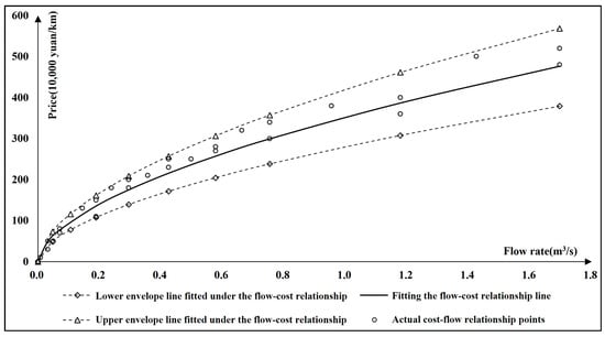
Figure 2.
Flow-cost-fitting curve for the water supply pipeline network.
Based on the scatter plot data, the relationship between flow and cost within the water supply network was analyzed and modeled using an exponential function fitted through the least squares method. This approach resulted in the following equation to describe the flow-cost relationship:
The index ‘K-hard’ is introduced to evaluate the complexity level of constructing the pipe network, with values ranging from 0 to 1. The cost of water supply network construction, represented as F3, is determined using the following equation:
In the equation above, d represents the length of the pipeline network (in kilometers), q represents the pipeline flow rate (m3/s), j represents the number of water demand nodes, and Route represents the shortest water supply path.
- 5.
- Pumping Station Construction Cost
The data on pumping station construction costs indicate that these expenses are roughly proportional to the station’s capacity, with an estimated cost of 2 million yuan for every 10,000 m3 per day of lifting capacity. This implies that building a new pumping station with a capacity of 10,000 m3 per day would involve an investment of approximately 2 million yuan. Accordingly, the pumping station construction cost, represented as F4, can be calculated using the following equation:
- 6.
- Water Treatment Plant Construction Cost
The existing project report on water treatment plant construction costs reveals that expenses are roughly proportional to the plant’s capacity, with an estimated cost of 10 million yuan for every 10,000 m3 per day of capacity. This means that building a new water treatment plant with a daily capacity of 10,000 m3 would require an investment of about 10 million yuan. Therefore, the construction cost of the water treatment plant, represented as F5, can be calculated using the following equation:
- 7.
- Water Intake Cost
Water intake costs encompass expenses for constructing intake structures and raw water transmission pipelines. Using unit cost data from multiple water intake projects reported in existing studies, a relationship between the scale of water intake and its associated costs has been identified. This relationship is depicted in a scatter plot and analyzed through a fitting process to derive a clear correlation. Furthermore, the upper and lower bounds of the scatter points have been determined, as shown in Figure 3.
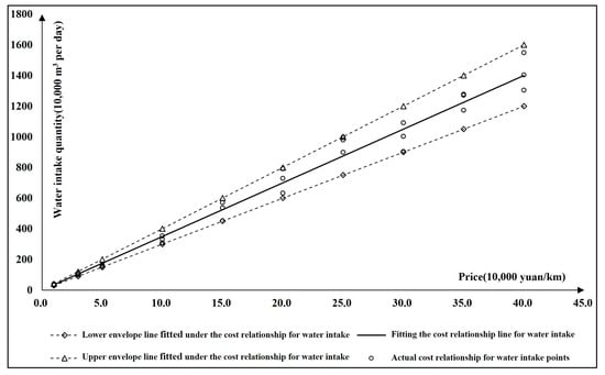
Figure 3.
Water-intake-cost-fitting curve.
Using the scatter plot data, the relationship between water intake and cost was modeled as a linear function, employing the least squares method for fitting analysis. The resulting water-intake-cost relationship is expressed by the following equation:
Based on the fitting results, the construction difficulty matrix for the extraction project, represented as Provide-hard, and the distance matrix for the extraction project, represented as Provide-dist, are introduced as the two key parameters defining the construction of the extraction project. The values of Provide-hard range between 0 and 1. The extraction cost, represented as F6, can be calculated using the following equation:
In the equation above, Provide-hard represents the construction difficulty matrix for the water intake project, while Provide-dist represents the distance matrix for the water intake project (km).
2.3.2. Constraint Conditions
- Water Quantity Constraint
- Water Supply Quantity Constraint at Supply Nodes
The water supply source is subject to an upper limit on its available supply capacity, constrained to be non-negative, with a lower bound of zero. This constraint on water supply capacity is represented by the following equation:
In the equation above, Cwater represents the matrix for water supply node quantity constraints; Lb-c represents the lower limit of the water supply node quantity constraint; Ub-c represents the upper limit of the water supply node quantity constraint; Ability pertains to the water supply capacity from the water plant (or water demand); Ewater corresponds to the water supply capacity provided by the water conservancy project; and Nwater refers to the incoming water conditions.
- Water Demand Constraint at Demand Nodes
In this study, only a lower limit is defined, while no upper limit is specified. The lower limit is determined based on water demand forecasting, which considers the requirements within the water supply system. By applying the quota method for calculating water demand, the constraints on water demand are represented by the following equation:
In the equation above, Dwater represents the matrix for water demand constraints at demand nodes; Lb-d represents the lower limit of the water demand constraints at demand nodes; pop represents the projected population for the planning year; and R-pop represents the water demand quota, set at 500 L per person per day.
- 2.
- Water Quality Constraint
According to Chinese government regulations, the initial chlorine concentration in water leaving the treatment plant must exceed 0.3 mg/L, while the residual chlorine concentration at the endpoints of the pipeline network should remain above 0.05 mg/L. As water is transmitted through the pipeline network, the residual chlorine concentration gradually diminishes, serving as a critical indicator of water quality within the network. This decay is influenced by factors such as time, temperature, turbidity, and pH. Extensive studies have addressed this issue, leading to the development of numerous models for predicting residual chlorine decay [47]. In this study, the optimization of chlorine decay processes is tailored to the characteristics of the allocation model. It involves fitting a simplified relationship between chlorine concentration and transmission distance, derived from measured data on chlorine decay along the transmission route, as illustrated in Figure 4.
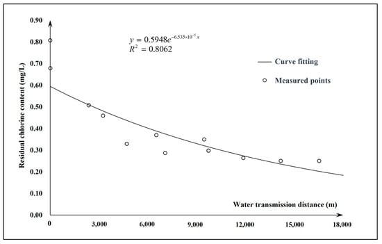
Figure 4.
Residual chlorine concentration decay curve along the transmission route.
The chlorine decay process is managed according to the following steps:
Initial Calculation: Determine the residual chlorine concentration along the route from the water supply node to the water demand node. If the concentration exceeds 0.05 mg/L, normal water supply continues.
Secondary Pressurization: If the residual chlorine concentration drops below 0.05 mg/L, apply secondary pressurization at the pumping station node. Update the transmission distance from the pumping station node to the water demand node to account for chlorine attenuation along the route. Recalculate the residual chlorine concentration. If the adjusted concentration exceeds 0.05 mg/L, water supply continues as planned.
Supply Infeasibility: If the recalculated concentration still does not meet the 0.05 mg/L threshold, the water supply node is considered unable to provide water to the water demand node (i.e., xij = 0).
Network-Wide Assessment: Repeat these steps for all combinations of water supply and water demand nodes to calculate the residual chlorine concentration throughout the entire network.
- 3.
- Water Pressure Constraint
In addition to maintaining water quality and quantity, the water supply system must also meet specific pressure requirements to ensure consistent access for users. To address this, the water supply model includes constraints related to water pressure. Low-pressure pipelines cannot pass through pumping station nodes or water treatment plants for pressurization, nor can they directly supply water to elevated areas. Alternatively, higher-elevation areas can supply water directly to lower-elevation areas. In practical calculations, these pressure constraints primarily impact the Route matrix, which defines the water supply paths, and the Dist matrix, which represents the supply distances. These constraints are handled using the graph theory methodology described in Step 1 of Section 2.2.
In summary, the optimization process incorporates nonlinear constraints inherent in multi-source urban water supply systems, including flow balance equations, pipeline losses, and water quality attenuation. These constraints are formulated within the graph-theoretic framework to ensure realistic simulation and optimization. For instance, the nonlinear relationship between flow rate and pipeline cost is addressed using the Pendershue formula, while flow balance constraints ensure that the inflow and outflow at each node remain consistent. These formulations are embedded into the optimization algorithm, enabling the model to handle the complexities of multi-source allocations effectively.
2.3.3. Model Solution
This model involves numerous variables during the optimization process, resulting in a complex discrete multivariate nonlinear optimization problem. To address these challenges, the model adopts the standard Genetic Algorithm (GA). However, due to the unique characteristics of this model and the inherent limitations of standard GA, several iterations and refinements were introduced to improve its performance. Consequently, an enhanced hybrid approach was developed, integrating Simulated Annealing (SA) and the Chaos Optimization Algorithm (COA), leveraging principles from previous research.
The GA process involves collective operations within the population, including selection, crossover, and mutation, which form the foundation of the iterative process [48]. All individuals in the population undergo parallel iterations. By intergrating SA and COA, an annealing strategy and a chaotic local fine search mechanism are applied simultaneously to all individuals [49,50]. During updates, suboptimal results are excluded, ensuring the progressive refinement of solutions and convergence.
The GA employs floating-point encoding for individuals, with random selection used as the selection operator and a default tournament size of 100. The population size is set to 100, and initial solutions are generated randomly and filtered to ensure feasibility. Too few random solutions may result in insufficient diversity, while too many may prolong computation time or produce suboptimal results. Debugging revealed that the optimal range of initial solutions was determined to be between 5000 and 200,000, depending on the number of variables. The default configuration is set at 20,000 solutions. The model executes 400 genetic iterations by default, using single-point crossover and real-number mutation operators. For the SA operator, the annealing and current temperatures correspond to the generations in GA, with adjustments made to the annealing function. Key parameters are pre-determined, including an initial acceptance probability of 0.4, a termination acceptance probability of 0.08, and an acceleration factor of 1. A larger acceleration factor leads to faster acceptance probability. Regarding COA, the adjustment parameter τ is set at 0.2 in this model. The overall solution process is depicted in Figure 5, with specific input file formats detailed in Section 4.2.
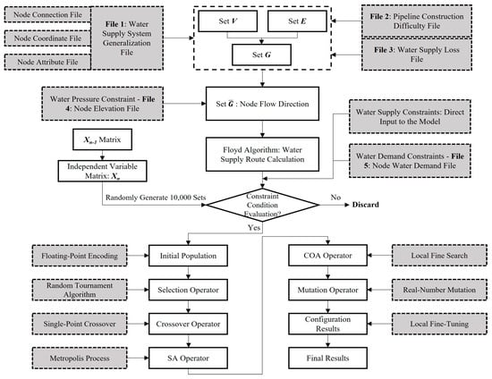
Figure 5.
The flow chart of model solution.
The optimization algorithm integrates Genetic Algorithm (GA), Chaos Optimization Algorithm (COA), and Simulated Annealing (SA) to achieve both high accuracy and efficiency in solving complex, multi-constraint optimization problems. GA serves as the foundational framework for exploring the solution space through selection, crossover, and mutation. However, GA alone is prone to premature convergence and may struggle with local optima in highly nonlinear scenarios. To address these limitations, COA introduces a chaotic mapping mechanism, enabling finer adjustments in local search areas and improving convergence precision. Meanwhile, SA incorporates a probabilistic annealing strategy to prevent premature convergence, allowing for the exploration of diverse solution paths and escaping local optima. This hybrid GA-COA-SA algorithm combines the strengths of global exploration and local refinement, accelerating convergence while delivering high-quality solutions that effectively handle the nonlinear constraints and complexities inherent in multi-source urban water supply systems.
2.3.4. Model Design and Development
The interface design and background calculations for this study were developed using MATLAB R2022a, which offers two primary methods for creating graphical user interfaces (GUIs). The first method involves directly coding interface parameters, such as icon positions and sizes, within an m-file. While functional, this method can be labor-intensive and difficult to debug, leading to lower development efficiency. The second method uses MATLAB’s GUI Guide tool, which links front-end graphical interface files with background calculations in m-files. This method simplifies both development and debugging processes, enhancing overall workflow efficiency. For proper operation during runtime, both the graphical interface file and the background m-file are required.
In this study, the GUI Guide method was selected to streamline the development process. The model consists of four main modules: file loading, parameter input, optimization solving, and result export. After debugging the graphical interface and background computations, the program was compiled into a standalone executable (.exe) file to allow it to run independently of the MATLAB environment. Although MATLAB includes its Lcc-win32 C compiler, a more stable option, Microsoft Visual C++ 2022, was used during the compilation process to enhance reliability. During the first compilation, the system prompts the user to choose a compiler type, and the decision to use an external compiler ensured smoother performance.
3. Case Study
Lishui City, located in eastern coastal China, is part of Zhejiang Province. It spans longitudes 118°45′ to 121°00′ E and latitudes 27°28′ to 28°48′ N. As of 2023, the city has a population of about 2.2 million [51], with the central urban area highlighted in red and its surrounding boundaries illustrated with gradient zones in Figure 6.

Figure 6.
Diagram of the urban water supply system of Lishui City.
Figure 6 shows that the central urban area of Lishui has a water supply capacity of 300,000 m3/d, supported by three water plants: the Tianning Water Plant, Shuige Water Plant, and Hucun Water Plant [51]. The Tianning Water Plant sources water from the Huangcun Reservoir, with a supply capacity of 100,000 m3/d. Similarly, the Shuige Water Plant relies on the Yuxi Reservoir and provides an equivalent capacity of 100,000 m3/d. The Hucun Water Plant, which sources water from the Tankeng Reservoir located outside the central urban area, also contributes 100,000 m3/d. The specific water transmission routes are illustrated in Figure 6, where the Tianning Water Plant and Shuige Water Plant, located within the central urban area, are represented by yellow lines. In contrast, the Hucun Water Plant, situated outside the central urban area, is represented by red lines.
Rapid population growth and increased economic activity in Lishui’s central urban area are placing significant pressure on its water supply system. According to the “Lishui City Water Resources Planning (2020–2030)” [52], the area’s water demand is expected to require a total supply capacity of 500,000 m3/d by 2030. To address this growing demand, expanding the existing water plants has become a pressing priority.
4. Results
4.1. Formulation of Water Diversion and Supply Plan
4.1.1. Water Diversion Plan
The Huangcun Reservoir faces operational limitations due to its restricted inflow and storage capacity, which confine it to its current supply level. Expanding its storage capacity would involve substantial financial investment and is further complicated by the dense population living nearby, making implementation both costly and socially challenging. Similarly, the water diversion pipeline from the Yuxi Reservoir is at risk of contamination due to the planned construction of an airport, which would require costly modifications to the existing pipeline [52]. In contrast, the Tankeng Reservoir offers significant advantages as a primary water source. With its abundant water volume and excellent water quality, it emerges as an optimal solution for meeting the region’s water supply needs. Based on this assessment, the following water diversion plans for the Tankeng Reservoir are proposed:
(1) Tankeng Water Diversion Plan 1: Divert water from the Tankeng Reservoir to the Hucun Water Plant.
(2) Tankeng Water Diversion Plan 2: Divert water from the Tankeng Reservoir to both the Hucun Water Plant and the Tianning Water Plant.
4.1.2. Water Supply Plan
Considering the existing water supply layout and the need to achieve a daily water supply capacity of 500,000 m3/d in Lishui’s urban area by 2030, three plans are proposed. These plans take into account economic costs, construction challenges, and other relevant factors:
(1) Plan 1: Restrict the operation of the Shuige Water Plant and increase the Tankeng Reservoir’s water diversion capacity to 300,000 m3/d. Of this, 200,000 m3/d will be supplied to the Tianning Water Plant, and 100,000 m3/d will be supplied to the Hucun Water Plant.
(2) Plan 2: Restrict the operation of the Shuige Water Plant and increase the Tankeng Reservoir’s water diversion capacity to 300,000 m3/d, with the entire volume supplied to the Hucun Water Plant.
(3) Plan 3: Gradually decommission the Shuige Water Plant and reroute its original supply line. The 100,000 m3/d originally supplied by the Yuxi Reservoir will be redirected to the Hucun Water Plant. Additionally, the Tankeng Reservoir’s water diversion capacity will be increased to 300,000 m3/d, supplying the Hucun Water Plant.
The layouts for these water diversion and supply plans are illustrated in Figure 7.
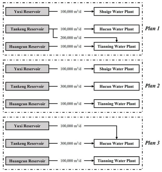
Figure 7.
The plans of water diversion and supply in 2030.
4.2. Model Input Files and Model Validation
4.2.1. Division and Generalization of Computational Units
The study area is divided into 12 water supply calculation units based on elevation, as illustrated in Figure 8a. Among these units, regions numbered 2, 3, 5, 6, 7, and 8 represent low-pressure water supply areas; regions numbered 1, 4, 9, 11, and 12 represent medium-pressure zones; and region number 10 represents the high-pressure zone. Building on this zoning, the water supply system is further generalized, as shown in Figure 8b, with the numbering in both figures corresponding to the same areas.
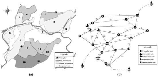
Figure 8.
(a) Schematic diagram of Lishui City water supply zones; (b) Generalized diagram of Lishui City water supply system.
4.2.2. Determination of Model Input Files
The files necessary for model input are detailed in Section 2.3.3. These input files are categorized into five main types: water supply system generalization files, pipeline construction difficulty files, water supply loss files, node elevation files, and node water demand files. The water supply system generalization files further comprise node connection files, node coordinate files, and node attribute files.
- Water Supply System Generalization Files
- Node Connection File
The connection relationships between two unit nodes are defined as shown in Table 1 and correspond to the generalized relationships depicted in Figure 8b.

Table 1.
Node connection file.
- Node Coordinate File
The latitude, longitude, and elevation of each unit node are provided to facilitate calculations in the water quantity allocation. The coordinates of each node are shown in Table 2.
Table 2.
Node coordinate file.
- Node Attribute File
Table 3 provides the attributes of each unit node. In this model, the attributes are categorized as water demand nodes, water supply nodes, intermediate nodes, and pumping station nodes, corresponding to 1, 2, 3, and 4, respectively.
Table 3.
Node attribute file.
- 2.
- Pipeline Construction Difficulty File
Table 4 defines the construction difficulty for different sections. A value of 1 indicates a challenging section, leading to higher costs. In this context, the difficulty for roads crossing the river in the generalized road nodes is assigned a value of 1. The road numbers correspond to the generalized relationships depicted in Figure 8b.
Table 4.
Pipeline construction difficulty file.
- 3.
- Water Supply Loss File
Water supply loss is primarily influenced by water pressure and supply distance. Considering the characteristics of the allocation model, a simplification is applied, treating it solely as a function of supply distance. It is important to note that a water supply loss of 0% does not signify the absence of actual loss but rather indicates that the node cannot directly supply water to the corresponding node without pressurization via a pumping station node; thus, it is forcibly set to 0%. The water supply loss for each node is detailed in Table 5.
Table 5.
Water supply loss file.
- 4.
- Node Elevation Attribute File
The node elevation attribute file categorizes nodes further based on their altitude. Numbers 1, 2, and 3 correspond to low, medium, and high elevation attributes, respectively. The elevation attributes for each node are shown in Table 6.
Table 6.
Node elevation attribute file.
- 5.
- Node Water Demand File
The node water demand file is established based on forecasted water demand for the planning year. For the proposed water supply system plan discussed earlier, the water demand for each node in 2023 and 2030 is provided in Table 7.
Table 7.
Water user constraint lower limit (using predicted water demand). Unit: 104 m3/d.
4.2.3. Model Validation
Before performing calculations, a validation is conducted for the baseline year to ensure the model’s accuracy and adjust specific constants within it. This simulation is then compared with the current water quantity plan. Table 8 presents the water quantity allocation plan for each subregion in the baseline year (2023), as determined by the water quantity allocation model developed in this study.
Table 8.
Comparison of current allocation and optimized allocation results. Unit: 104 m3/d.
In terms of the allocation plan, differences between the two plans are observed only at Node 5 and Node 7. Although the Tianning Water Plant supplies Area 5 in the current allocation plan, which involves a shorter distance, it requires crossing the Oujiang River, leading to higher costs. The optimized allocation plan calculated based on the model in this study addresses these inefficiencies, achieving a more cost-effective distribution by reallocating resources to minimize operational costs. Specifically, the annual cost under the optimized allocation is 4.6319 × 10⁷ yuan, compared to 4.6978 × 10⁷ yuan in the current allocation, reflecting a cost reduction of approximately 0.0659 × 10⁷ yuan annually. This represents a 1.4% improvement in economic efficiency, highlighting the practical benefits of the optimization model in fine-tuning resource allocation to achieve measurable economic gains. These results align closely with actual conditions, further demonstrating the reliability and reasonableness of the optimization model’s outcomes. All parameters in this allocation plan calculation use default settings, consistent with the settings applied for the planned year discussed later.
4.3. Model Calculation Results
4.3.1. Subregion Allocation Calculation Results
Using the water quantity optimization allocation model established in this study, three plans were calculated for 2030. The combined water supply calculation results for each plan are shown below, as presented in Table 9, Table 10 and Table 11.
Table 9.
Statistical table of water quantity optimization allocation model for each subregion in 2030 under Plan 1. Unit: 104 m3/d.
Table 10.
Statistical table of water quantity optimization allocation model for each subregion in 2030 under Plan 2. Unit: 104 m3/d.
Table 11.
Statistical table of water quantity optimization allocation model for each subregion in 2030 under Plan 3. Unit: 104 m3/d.
4.3.2. Road Node Water Supply Capacity
The road node water supply capacity for each plan is detailed in Appendix A (Table A1) due to the extensive data volume, which makes it more appropriate to include this supplementary information in the appendix for reference.
4.3.3. Annual Operating Cost Optimization Results for Water Supply
The equivalent annual cost increments after optimization for each plan, along with the cumulative incremental costs leading to the average annual cost for 2030, are presented in Table 12.
Table 12.
Statistical table of annual cost increments and total annual costs for each plan. Unit: 104 yuan.
4.4. Results Analysis
This section presents a comprehensive analysis of the outcomes derived from the graph-theory-based optimization model for multi-source urban water supply systems. The findings are structured into four main areas. First, the Water Supply Analysis evaluates the supply capacities of the three proposed allocation plans, accounting for pipeline losses and supply reliability. Second, the Cost Analysis examines the financial implications of each plan, emphasizing annual costs and the balance between supply efficiency and cost minimization. Notably, the analysis highlights that the proposed model achieves a measurable improvement in economic efficiency compared to the current allocation strategy, providing a more cost-effective framework for future water supply planning. Third, the Comprehensive Evaluation integrates results from the supply and cost analyses, providing a holistic assessment to identify the optimal strategy for Lishui City. Finally, a Comparative Perspective with Traditional Models highlights the advantages of the proposed model over conventional optimization approaches, demonstrating its ability to address real-world complexities and constraints effectively. Collectively, these analyses underline the adaptability, efficiency, and broader applicability of the proposed model in urban water resource management, particularly in enhancing cost-effectiveness and planning for future scenarios.
4.4.1. Water Supply Analysis
The three proposed plans were analyzed based on the projected 2030 water demand, focusing on their water supply strategies, pipeline losses, and operational efficiency. Although all plans are designed to achieve the same theoretical supply capacity of 40.05 × 10⁴ m3/d (excluding pipeline losses, as shown in Table 9), the net water supplied after losses varies significantly, highlighting the strengths and trade-offs of each plan.
Plan 1 employs a distributed allocation strategy, with water supply divided among the Tianning, Shuige, and Hucun water plants. After accounting for pipeline losses, the actual supply volume is 43.87 × 10⁴ m3/d (Table 9), indicating the lowest water loss of 3.82 × 10⁴ m3/d among the three plans. This efficiency is primarily due to shorter pipeline routes and a more balanced distribution of supply nodes, minimizing water loss. However, the reliance on multiple plants increases management complexity and operational costs.
Plan 2 prioritizes water supply to Hucun from the Tankeng Reservoir, reducing dependence on the Tianning and Shuige plants. The net supply volume after losses rises to 45.92 × 10⁴ m3/d (Table 10), resulting in a moderate loss of 5.87 × 10⁴ m3/d compared to the other plans. The plan’s simplified network structure improves efficiency, but longer pipeline routes contribute to higher water losses. Additionally, reduced system redundancy limits adaptability during potential disruptions.
Plan 3 consolidates the water supply by phasing out the Shuige Water Plant and using the Tankeng Reservoir as the dominant source. This plan achieves the highest net supply of 47.40 × 10⁴ m3/d (Table 11), but it also indicating the highest loss of 7.35 × 10⁴ m3/d compared to the original supply capacity. Despite these losses, the plan incorporates ecological water supply components, leveraging the high-quality water of the Tankeng Reservoir. The reduced reliance on multiple plants simplifies operations, but the system’s stability may be affected due to its dependency on fewer water treatment plants.
As summarized in Table A1, Plan 1 demonstrates the lowest pipeline loss, making it the most efficient from a water conservation perspective. However, its distributed structure results in higher operational and management complexity. Plan 2 balances simplicity and moderate pipeline losses, making it a more streamlined option but with reduced flexibility. Plan 3 stands out for its ability to supply the highest volume of high-quality water, including ecological benefits, although it incurs the highest pipeline losses and relies heavily on the Tankeng Reservoir, potentially affecting system resilience.
4.4.2. Cost Analysis
The economic analysis of the three plans, summarized in Table 12, highlights the trade-offs between cost efficiency and system resilience.
Plan 1, with the highest annual cost of 6.2022 × 10⁷ yuan, reflects the financial burden of its multi-plant supply strategy. This approach effectively distributes the supply load across the Tianning, Shuige, and Hucun water plants, enhancing redundancy and system resilience. However, it requires significant investment in inter-plant coordination and complex infrastructure, which drives up overall expenses and operational challenges.
Plan 2 emerges as the most economical option, with an annual cost of 5.7015 × 10⁷ yuan, the lowest among the three plans. Its simplified routing system reduces both operational and infrastructure expenses, making it a highly cost-efficient choice. However, this cost advantage is achieved at the expense of flexibility and system resilience. The reliance on longer pipelines in Plan 2 increases water losses, which could impact supply efficiency and adaptability during unexpected disruptions.
Plan 3 offers a balanced solution, with an annual cost of 5.9246 × 10⁷ yuan, sitting between Plans 1 and 2. By consolidating supply through the Tankeng Reservoir and reallocating resources from the decommissioned Shuige Water Plant, it combines moderate cost efficiency with operational scalability. However, its reliance on the Tankeng Reservoir as the primary source introduces risks of supply disruption, which may challenge long-term system stability.
In conclusion, Plan 2 stands out for its superior cost-efficiency, making it a financially attractive choice for urban water supply planning, especially in scenarios prioritizing budget constraints. However, its limitations in flexibility and resilience should be carefully considered in the context of long-term operational demands. While Plan 3 provides a good compromise between cost and scalability, its reliance on a single dominant source highlights potential vulnerability.
4.4.3. Comprehensive Evaluation
The comprehensive analysis of the three proposed plans reveals significant differences in water allocation strategies, supply capacities, and associated costs.
Plan 1 distributes the water supply among the Tianning, Shuige, and Hucun water plants, achieving a supply volume of 43.87 × 10⁴ m3/d after accounting for pipeline losses. This approach effectively reduces the operational burden on individual plants and enhances redundancy, contributing to greater resilience. However, it requires extensive cross-plant coordination and incurs the highest annual cost of 6.2022 × 10⁷ yuan. These high costs reflect significant investments in infrastructure and the complexities of managing a distributed system.
Plan 2 focuses most of the supply on the Hucun Water Plant from the Tankeng Reservoir, simplifying the system and achieving a higher supply volume of 45.92 × 10⁴ m3/d. This plan demonstrates exceptional cost efficiency, with the lowest annual cost of 5.7015 × 10⁷ yuan, making it the most economical choice among the three. However, its reliance on extended pipelines results in increased water losses, and the limited number of backup options reduces system flexibility and resilience during potential disruptions.
Plan 3 phases out the Shuige Water Plant and consolidates supply through the Tankeng Reservoir. This plan achieves the highest supply capacity of 47.40 × 10⁴ m3/d despite experiencing the largest pipeline losses. With a moderate annual cost of 5.9246 × 10⁷ yuan, it offers a balance between cost and capacity. Plan 3 leverages Tankeng’s ample, high-quality water resources and simplifies system dependencies. However, its reliance on a single dominant source introduces potential vulnerabilities to supply disruptions, posing risks to long-term reliability.
Among the three plans, Plan 2 emerges as the most cost-effective option, achieving the lowest annual cost while delivering a supply volume of 45.92 × 10⁴ m3/d, which is higher than Plan 1. Although it sacrifices some flexibility and resilience due to increased water losses and fewer backup options, its strong economic performance makes it the most practical choice for immediate implementation. While Plan 3 offers the greatest supply capacity and moderate costs, its dependency on a single source increases risk, and Plan 1, though resilient, is less feasible due to its high costs. Plan 2 is the optimal solution for current conditions, balancing supply efficiency and cost-effectiveness. Moving forward, future studies could explore methods to mitigate water losses and enhance flexibility, such as optimizing pipeline routes or incorporating secondary backup systems. Additionally, integrating environmental sustainability and dynamic management strategies will further strengthen long-term urban water supply planning.
4.4.4. Comparative Perspective with Traditional Models
Traditional optimization models, such as linear programming (LP), are widely used in water resource management due to their simplicity and computational efficiency. These models excel in solving single-objective optimization problems, such as minimizing supply-demand gaps or operational costs, under predefined constraints. However, their applicability diminishes when addressing the complexities of multi-source urban water supply systems, particularly under dynamic conditions involving pipeline losses, water quality attenuation, and pressure variations. LP models generally treat water distribution as a linear allocation problem, which limits their ability to represent the structural and hydraulic interconnections within supply networks.
In contrast, the proposed graph-theory-based optimization model provides a more comprehensive and adaptable framework. By representing the water supply system as a network of interconnected nodes and edges, this model captures the intricate flow paths and interactions within the supply network. Unlike LP models, the graph-theoretic approach directly integrates dynamic constraints such as flow balance, pipeline losses, and water quality attenuation, ensuring a more accurate simulation and optimization under real-world conditions. Furthermore, it excels in handling multi-source allocations by effectively coordinating supply from multiple reservoirs or plants, making it particularly well-suited for complex, large-scale systems such as those found in urban areas.
While LP models remain effective for simpler and small-scale problems, their limitations in addressing nonlinear dynamics and interconnected systems underscore the need for more advanced methods. The graph-theoretic model bridges this gap by offering a holistic approach that enhances both operational efficiency and adaptability. This study demonstrates the model’s practical advantages, including its ability to reduce costs and improve allocation efficiency in a real-world case study. Future research could extend the graph-theoretic framework to incorporate multi-objective optimization, balancing factors such as cost-efficiency, ecological sustainability, and supply reliability, further enhancing its relevance and applicability to diverse urban contexts and advancing sustainable water resource management.
5. Discussion
This study underscores the advantages of using graph-theoretic approaches to optimize urban multi-source water supply systems. Unlike traditional single-source frameworks, the proposed model leverages the structural flexibility of multi-source systems to enhance resilience and meet fluctuating supply and demand conditions. By incorporating graph theory, the model effectively captures complex interconnections and flow paths, enabling simultaneous optimization of water distribution and operational costs. Compared to traditional methods such as linear programming or heuristic approaches, the graph-theoretic framework offers superior adaptability to multi-source configurations while addressing critical challenges like water quality, pressure, and connectivity.
A key innovation of this study lies in the integration of the GA-COA-SA algorithm, which combines the global exploration capabilities of Genetic Algorithms (GA) with the fine-tuning precision of Chaos Optimization Algorithm (COA) and the probabilistic annealing strategy of Simulated Annealing (SA). This hybrid approach significantly improves convergence and computational efficiency, providing high-quality solutions for complex, multi-constraint scenarios. By effectively combining global and local optimization techniques, the algorithm overcomes challenges such as premature convergence and local optima, making it particularly suited to real-world urban water management.
The findings highlight the model’s ability to improve economic efficiency, achieving an annual cost reduction of approximately 0.0659 × 10⁷ yuan, representing a 1.4% improvement in cost-effectiveness. This is especially significant given the financial constraints identified by water authorities. By directly addressing these economic priorities, the model bridges the gap between theoretical optimization and practical application, ensuring its immediate relevance to stakeholders. While ecological sustainability and system resilience remain important considerations, this cost-focused approach enhances its applicability to the specific needs of Zhejiang Province.
However, the study has limitations. The reliance on static parameters reduces the model’s responsiveness to real-time changes in water demand and supply, and broader objectives, such as ecological impacts and long-term sustainability, are not fully addressed. Future research should focus on integrating multi-objective optimization frameworks and adaptive algorithms, enabling a balance among cost-efficiency, environmental sustainability, and system resilience. These advancements would further enhance the model’s robustness and applicability, paving the way for more sustainable and resilient urban water management strategies tailored to diverse contexts.
6. Conclusions
This study explores optimizing urban multi-source water supply systems by lever-aging graph theory and advanced optimization techniques to address challenges in water allocation, cost efficiency, and system resilience. Traditional single-source models often fail to meet the growing demands and reliability needs of modern urban systems under variable conditions. Applying the proposed graph-theory-based optimization model to Lishui City, the study highlights significant improvements in supply efficiency and cost management, achieving a 1.4% improvement in cost-effectiveness compared to the current allocation strategy. Plan 2 emerges as the most cost-effective solution, achieving a supply capacity of 45.92 × 10⁴ m3/d while maintaining the lowest annual cost of 5.7015 × 10⁷ yuan. This plan prioritizes cost efficiency by focusing water allocation through a simplified routing system, reducing operational and infrastructure expenses while balancing economic feasibility. The model integrates shortest path algorithms and considers constraints related to water quality, pressure, and connectivity, effectively capturing the complexities of multi-source allocations and enabling informed decision-making. The optimization process is further refined using the GA-COA-SA algorithm, which enhances solution precision and convergence through its combined methodologies. Compared to traditional linear programming and heuristic methods, the proposed approach offers greater adaptability and computational efficiency, bridging the gap between theoretical models and practical applications. Despite its advancements, the model relies on static parameters and lacks real-time adaptability, limiting its responsiveness to dynamic changes in demand and supply. Future research should explore the integration of adaptive algorithms and real-time monitoring to enhance flexibility and ensure applicability across diverse urban contexts. Additionally, extending the model to include multi-objective optimization frameworks could address broader concerns such as ecological impacts and system resilience, aligning with the evolving priorities of sustainable urban water management. The findings underscore the potential of graph-theoretic approaches combined with advanced optimization techniques to support sustainable urban development, optimize resources, and strengthen resilience in urban water management. By addressing key limitations and refining the model’s adaptability, this approach provides a robust foundation for future innovations in urban water supply system optimization.
Author Contributions
Conceptualization, J.Z. and X.Z.; methodology, J.Z.; software, J.Z.; validation, J.Z., Z.M. and H.L.; formal analysis, D.L.; investigation, X.Z.; resources, H.L.; writing—original draft preparation, J.Z.; writing—review and editing, Z.M.; visualization, Y.F.; supervision, S.P.; funding acquisition, J.Z. and D.L. All authors have read and agreed to the published version of the manuscript.
Funding
This research was funded by the General Projects of Zhejiang Provincial Education Department (No. Y202250299), the Joint Funds of Zhejiang Provincial Natural Science Foundation of China (No. LZJWY22E090003).
Data Availability Statement
Data are contained within the article.
Acknowledgments
The authors are particularly grateful to the Lishui Water Resources Bureau for providing the data sources.
Conflicts of Interest
The authors declare no conflicts of interest.
Appendix A
Table A1.
Statistical table of road node water supply capacity for each plan.
Table A1.
Statistical table of road node water supply capacity for each plan.
| Road Number | Plan 1 | Plan 2 | Plan 3 | ||||||
|---|---|---|---|---|---|---|---|---|---|
| Road Water Supply Volume 1 | Flow Rate 2 | Equivalent Pipe Diameter 3 | Road Water Supply Volume | Flow Rate | Equivalent Pipe Diameter | Road Water Supply Volume | Flow Rate | Equivalent Pipe Diameter | |
| 1 | 762.206 | 0.242 | 423.598 | 697.187 | 0.221 | 407.717 | 762.206 | 0.242 | 423.598 |
| 2 | 2922.304 | 0.927 | 753.514 | 2877.774 | 0.913 | 748.571 | 2922.304 | 0.927 | 753.514 |
| 3 | 600 | 0.19 | 382.311 | 600 | 0.19 | 382.311 | 600 | 0.19 | 382.311 |
| 4 | 724.684 | 0.23 | 414.532 | 884.103 | 0.28 | 451.406 | 724.684 | 0.23 | 414.532 |
| 5 | 1560.083 | 0.495 | 575.801 | 2637.855 | 0.836 | 721.158 | 1560.083 | 0.495 | 575.801 |
| 6 | 4186.394 | 1.327 | 879.017 | 3380.511 | 1.072 | 802.05 | 4186.394 | 1.327 | 879.017 |
| 7 | 1597.36 | 0.507 | 581.657 | 1597.36 | 0.507 | 581.657 | 1597.36 | 0.507 | 581.657 |
| 8 | 1192.601 | 0.378 | 513.19 | 3112.464 | 0.987 | 774.15 | 1192.601 | 0.378 | 513.19 |
| 9 | 748.336 | 0.237 | 420.277 | 600 | 0.19 | 382.311 | 748.336 | 0.237 | 420.277 |
| 10 | 3572.293 | 1.133 | 821.243 | 3233.683 | 1.025 | 786.93 | 3572.293 | 1.133 | 821.243 |
| 11 | 0 | 0 | 0 | 0 | 0 | 0 | 0 | 0 | 0 |
| 12 | 996.41 | 0.316 | 475.144 | 1820.218 | 0.577 | 615.143 | 996.41 | 0.316 | 475.144 |
| 13 | 600 | 0.19 | 382.311 | 600 | 0.19 | 382.311 | 600 | 0.19 | 382.311 |
| 14 | 1091.436 | 0.346 | 494.06 | 659.592 | 0.209 | 398.145 | 1091.436 | 0.346 | 494.06 |
| 15 | 0 | 0 | 0 | 0 | 0 | 0 | 0 | 0 | 0 |
| 16 | 0 | 0 | 0 | 600 | 0.19 | 382.311 | 0 | 0 | 0 |
| 17 | 600 | 0.19 | 382.311 | 600 | 0.19 | 382.311 | 600 | 0.19 | 382.311 |
| 18 | 0 | 0 | 0 | 0 | 0 | 0 | 0 | 0 | 0 |
| 19 | 600 | 0.19 | 382.311 | 828.514 | 0.263 | 439.016 | 600 | 0.19 | 382.311 |
| 20 | 600 | 0.19 | 382.311 | 600 | 0.19 | 382.311 | 600 | 0.19 | 382.311 |
| 21 | 748.336 | 0.237 | 420.277 | 600 | 0.19 | 382.311 | 748.336 | 0.237 | 420.277 |
| 22 | 996.41 | 0.316 | 475.144 | 1820.218 | 0.577 | 615.143 | 996.41 | 0.316 | 475.144 |
| 23 | 4776.828 | 1.515 | 930.153 | 4209.91 | 1.335 | 881.13 | 4776.828 | 1.515 | 930.153 |
| 24 | 912.683 | 0.289 | 457.603 | 3369.936 | 1.069 | 800.973 | 912.683 | 0.289 | 457.603 |
| 25 | 1304.596 | 0.414 | 533.316 | 634.005 | 0.201 | 391.451 | 1304.596 | 0.414 | 533.316 |
| 26 | 0 | 0 | 0 | 0 | 0 | 0 | 0 | 0 | 0 |
| 27 | 600 | 0.19 | 382.311 | 828.514 | 0.263 | 439.016 | 600 | 0.19 | 382.311 |
| 28 | 0 | 0 | 0 | 0 | 0 | 0 | 0 | 0 | 0 |
| 29 | 1596.414 | 0.506 | 581.51 | 600 | 0.19 | 382.311 | 1596.414 | 0.506 | 581.51 |
| 30 | 0 | 0 | 0 | 0 | 0 | 0 | 0 | 0 | 0 |
| 31 | 0 | 0 | 0 | 0 | 0 | 0 | 0 | 0 | 0 |
| 32 | 0 | 0 | 0 | 600 | 0.19 | 382.311 | 0 | 0 | 0 |
| 33 | 0 | 0 | 0 | 600 | 0.19 | 382.311 | 0 | 0 | 0 |
| 34 | 0 | 0 | 0 | 600 | 0.19 | 382.311 | 0 | 0 | 0 |
Notes: 1 The unit for road water supply volume is 104 m3 per year. 2 The unit for flow rate is m3/s. 3 The unit for equivalent pipe diameter is mm.
References
- Li, M.; Finlayson, B.; Webber, M.; Barnett, J.; Webber, S.; Rogers, S.; Chen, Z.; Wei, T.; Chen, J.; Wu, X.; et al. Estimating Urban Water Demand under Conditions of Rapid Growth: The Case of Shanghai. Reg. Environ. Change 2017, 17, 1153–1161. [Google Scholar] [CrossRef]
- Mishra, B.K.; Kumar, P.; Saraswat, C.; Chakraborty, S.; Gautam, A. Water Security in a Changing Environment: Concept, Challenges and Solutions. Water 2021, 13, 490. [Google Scholar] [CrossRef]
- Yang, J.; Cao, X.; Yao, J.; Zhang, Y.; Liu, Y.; Zhang, Y.; Li, X. Geographical Big Data and Data Mining: A New Opportunity for “Water-Energy-Food” Nexus Analysis. J. Geogr. Sci. 2024, 34, 203–228. [Google Scholar] [CrossRef]
- Handmer, J.; Honda, Y.; Kundzewicz, Z.W.; Arnell, N.; Benito, G.; Hatfield, J.; Mohamed, I.F.; Peduzzi, P.; Wu, S.; Sherstyukov, B.; et al. Changes in Impacts of Climate Extremes: Human Systems and Ecosystems. In Managing the Risks of Extreme Events and Disasters to Advance Climate Change Adaptation; Field, C.B., Barros, V., Stocker, T.F., Qin, D., Eds.; Cambridge University Press: Cambridge, UK, 2012; pp. 231–290. [Google Scholar] [CrossRef]
- Zhang, J.; Tang, D.; Wang, M.; Ahmad, I.; Hu, J.; Meng, Z.; Liu, D.; Pan, S. A Regional Water Resource Allocation Model Based on the Human–Water Harmony Theory in the Yellow River Basin. Water 2023, 15, 1388. [Google Scholar] [CrossRef]
- MacBroom, J.G.; Schiff, R. Predicting the Hydrologic Response of Salt Marshes to Tidal Restoration. In Tidal Marsh Restoration; Roman, C.T., Burdick, D.M., Eds.; Island Press: Washington, DC, USA, 2012; pp. 13–38. [Google Scholar] [CrossRef]
- Moore, I.D.; Turner, A.K.; Wilson, J.P.; Jenson, S.K.; Band, L.E. GIS and Land-Surface-Subsurface Process Modeling. In Environmental Modeling with GIS; Goodchild, M.F., Parks, B.O., Steyaert, L.T., Eds.; Oxford University Press: New York, NY, USA, 1993; pp. 196–230. [Google Scholar]
- Ateş, S. Hydraulic Modelling of Control Devices in Loop Equations of Water Distribution Networks. Flow Meas. Instrum. 2017, 53, 243–260. [Google Scholar] [CrossRef]
- Yoo, D.G.; Lee, J.H.; Lee, B.Y. Comparative Study of Hydraulic Simulation Techniques for Water Supply Networks under Earthquake Hazard. Water 2019, 11, 333. [Google Scholar] [CrossRef]
- Shuang, Q.; Liu, H.J.; Porse, E. Review of the Quantitative Resilience Methods in Water Distribution Networks. Water 2019, 11, 1189. [Google Scholar] [CrossRef]
- Lachowicz, M. Microscopic, Mesoscopic and Macroscopic Descriptions of Complex Systems. Probabilistic Eng. Mech. 2011, 26, 54–60. [Google Scholar] [CrossRef]
- Lützenkirchen, J.; Preočanin, T.; Kallay, N. A Macroscopic Water Structure Based Model for Describing Charging Phenomena at Inert Hydrophobic Surfaces in Aqueous Electrolyte Solutions. Phys. Chem. Chem. Phys. 2008, 10, 4946–4955. [Google Scholar] [CrossRef]
- Hailemariam, F.M.; Brandimarte, L.; Dottori, F.; Di Baldassarre, G. Investigating the Influence of Minor Hydraulic Structures on Modeling Flood Events in Lowland Areas. Hydrol. Process. 2014, 28, 1742–1755. [Google Scholar] [CrossRef]
- Jamaloei, B.Y. A Critical Review of Common Models in Hydraulic-Fracturing Simulation: A Practical Guide for Practitioners. Theor. Appl. Fract. Mech. 2021, 113, 102937. [Google Scholar] [CrossRef]
- Tong, L.; Cai, Y.; Liu, Q. Carbonation Modelling of Hardened Cementitious Materials Considering Pore Structure Characteristics: A Review. J. Build. Eng. 2024, 71, 110547. [Google Scholar] [CrossRef]
- Vilanova, M.R.N.; Balestieri, J.A.P. Modeling of Hydraulic and Energy Efficiency Indicators for Water Supply Systems. Renew. Sustain. Energy Rev. 2015, 48, 540–557. [Google Scholar] [CrossRef]
- van der Heijde, B.; Fuchs, M.; Tugores, C.R.; Schweiger, G. Dynamic Equation-Based Thermo-Hydraulic Pipe Model for District Heating and Cooling Systems. Energy Convers. Manag. 2017, 151, 158–169. [Google Scholar] [CrossRef]
- Gupta, R.S. Hydrology and Hydraulic Systems; Waveland Press: Long Grove, IL, USA, 2016. [Google Scholar]
- Sitkoff, D.; Sharp, K.A.; Honig, B. Accurate Calculation of Hydration Free Energies Using Macroscopic Solvent Models. J. Phys. Chem. 1994, 98, 1978–1988. [Google Scholar] [CrossRef]
- Leclercq, L.; Chiabaut, N.; Trinquier, B. Macroscopic Fundamental Diagrams: A Cross-Comparison of Estimation Methods. Transp. Res. Part B Methodol. 2014, 62, 1–12. [Google Scholar] [CrossRef]
- Xing, J.; Wu, W.; Cheng, Q.; Zhang, W.; Zhang, J. Traffic State Estimation of Urban Road Networks by Multi-Source Data Fusion: Review and New Insights. Phys. A Stat. Mech. Appl. 2022, 595, 127079. [Google Scholar] [CrossRef]
- Afyouni, I.; Al Aghbari, Z.; Razack, R.A. Multi-Feature, Multi-Modal, and Multi-Source Social Event Detection: A Comprehensive Survey. Inf. Fusion 2022, 79, 279–308. [Google Scholar] [CrossRef]
- Cullen, A.C.; Rubinstein, B.I.P.; Kandeepan, S.; Wang, Z.; Lin, C. Predicting Dynamic Spectrum Allocation: A Review Covering Simulation, Modelling, and Prediction. Artif. Intell. Rev. 2023, 56, 10921–10959. [Google Scholar] [CrossRef]
- Durlik, I.; Miller, T.; Cembrowska-Lech, D.; Wojciechowski, M.; Polap, D. Navigating the Sea of Data: A Comprehensive Review on Data Analysis in Maritime IoT Applications. Appl. Sci. 2023, 13, 9742. [Google Scholar] [CrossRef]
- Chen, H.; Xu, B.; Qiu, H.; Huang, S.; Teegavarapu, R.S.; Xu, Y.P.; Xie, H. Adaptive Assessment of Reservoir Scheduling to Hydrometeorological Comprehensive Dry and Wet Condition Evolution in a Multi-Reservoir Region of Southeastern China. J. Hydrol. 2024, 648, 132392. [Google Scholar] [CrossRef]
- Zhou, T.; Dong, Z.; Wang, W.; Cui, L.; Lin, G. Study on Multi-Scale Coupled Ecological Dispatching Model Based on the Decomposition-Coordination Principle. Water 2019, 11, 1443. [Google Scholar] [CrossRef]
- Wang, L.; Liu, H. An Efficient Method for Identifying and Filling Surface Depressions in Digital Elevation Models for Hydrologic Analysis and Modeling. Int. J. Geogr. Inf. Sci. 2006, 20, 193–213. [Google Scholar] [CrossRef]
- Yamazaki, D.; Oki, T.; Kanae, S. Deriving a Global River Network Map and Its Sub-Grid Topographic Characteristics from a Fine-Resolution Flow Direction Map. Hydrol. Earth Syst. Sci. 2009, 13, 2241–2251. [Google Scholar] [CrossRef]
- Pagano, A.; Sweetapple, C.; Farmani, R.; Giordano, R.; Butler, D. Water Distribution Networks Resilience Analysis: A Comparison between Approaches and Global Resilience Analysis. Water Resour. Manag. 2019, 33, 2925–2940. [Google Scholar] [CrossRef]
- Lu, L.; Wang, L.; Yang, Q.; Zhao, P.; Du, Y.; Xiao, F.; Ling, F. Extracting a Connected River Network from DEM by Incorporating Surface River Occurrence Data and Sentinel-2 Imagery in the Danjiangkou Reservoir Area. Remote Sens. 2023, 15, 1014. [Google Scholar] [CrossRef]
- Qiao, Z.; Ma, L.; Liu, T.; Wang, H.; Zhao, H. An Ecological Stability-Oriented Model for the Conjunctive Allocation of Surface Water and Groundwater in Oases in Arid Inland River Basins. Water Supply 2021, 21, 368–385. [Google Scholar] [CrossRef]
- Fan, Y.; Chen, H.; Gao, Z.; Ren, X.; Yang, J. A Model Coupling Water Resource Allocation and Canal Optimization for Water Distribution. Water Resour. Manag. 2023, 37, 1341–1365. [Google Scholar] [CrossRef]
- Bello, O.; Abu-Mahfouz, A.M.; Hamam, Y.; Munda, J.L.; Mpholo, M. Solving Management Problems in Water Distribution Networks: A Survey of Approaches and Mathematical Models. Water 2019, 11, 562. [Google Scholar] [CrossRef]
- Chen, C.; Wang, Z.; Wu, J.; Zhang, L.; Zhao, X. Interactive Graph Construction for Graph-Based Semi-Supervised Learning. IEEE Trans. Vis. Comput. Graph. 2021, 27, 3701–3716. [Google Scholar] [CrossRef]
- Shaikh, P.W.; El-Abd, M.; Khanafer, M.; Ahmed, E.; Shah, A. A Review on Swarm Intelligence and Evolutionary Algorithms for Solving the Traffic Signal Control Problem. IEEE Trans. Intell. Transp. Syst. 2020, 23, 48–63. [Google Scholar] [CrossRef]
- Alqaisi, R.; Ghanem, W.; Qaroush, A. Extractive Multi-Document Arabic Text Summarization Using Evolutionary Multi-Objective Optimization with K-Medoid Clustering. IEEE Access 2020, 8, 228206–228224. [Google Scholar] [CrossRef]
- Deep, A.; Dash, P.K. Applications of Cuckoo Search Algorithm for Optimization Problems. In Nature-Inspired Algorithms Applications; Springer: Cham, Switzerland, 2021; pp. 295–315. [Google Scholar] [CrossRef]
- Yazdani, A.; Jeffrey, P. Applying Network Theory to Quantify the Redundancy and Structural Robustness of Water Distribution Systems. J. Water Resour. Plan. Manag. 2012, 138, 153–161. [Google Scholar] [CrossRef]
- Sitzenfrei, R. Using Complex Network Analysis for Water Quality Assessment in Large Water Distribution Systems. Water Res. 2021, 201, 117359. [Google Scholar] [CrossRef]
- Marsili, V.; Alvisi, S.; Maietta, F.; Capponi, C.; Meniconi, S.; Brunone, B.; Franchini, M. Extending the Application of Connectivity Metrics for Characterizing the Dynamic Behavior of Water Distribution Networks. Water Resour. Res. 2023, 59, e2023WR035031. [Google Scholar] [CrossRef]
- Zhang, H.; Fu, G.; Kapelan, Z.; Wang, H. Optimizing Multi-Objective Water Distribution System Design Using Evolutionary Algorithms and Graph-Based Measures. J. Water Resour. Plan. Manag. 2022, 148, 04021099. [Google Scholar] [CrossRef]
- Ebrahimi, A.; Khamehchi, E. A New Hybrid Particle Swarm Optimization and Genetic Algorithm Method Controlled by Fuzzy Logic. IEEE Access 2019, 7, 115768–115781. [Google Scholar] [CrossRef]
- Jahandideh-Tehrani, M.; Hekmatnia, A.; Hashemi, M.; Javadi, S. Application of Particle Swarm Optimization to Water Management: An Overview. Environ. Monit. Assess. 2020, 192, 204. [Google Scholar] [CrossRef]
- Mandal, S.; Chakraborty, S. Hybrid Optimization Algorithms of Firefly with GA and PSO for the Least Cost Design of Water Distribution Networks. Water 2023, 15, 1906. [Google Scholar] [CrossRef]
- Rani, D.; Moreira, M. Simulation-Based Optimization of Water Resource Systems: A Review. Water Resour. Manag. 2024, 11, 1–24. [Google Scholar] [CrossRef]
- Zhang, H.; Liu, G.; Wang, R.; Yu, J.; Chen, X. A Hybrid Particle Swarm Optimization-Genetic Algorithm for Ecological Dispatching Models Considering Different Ecological Flow Requirements. Water Resour. Manag. 2024, 38, 2229–2249. [Google Scholar] [CrossRef]
- Monteiro, L.; Carneiro, J.; Covas, D.I.C. Modelling Chlorine Wall Decay in a Full-Scale Water Supply System. Urban Water J. 2020, 17, 754–762. [Google Scholar] [CrossRef]
- Katoch, S.; Chauhan, S.S.; Kumar, V. A Review on Genetic Algorithm: Past, Present, and Future. Multimed. Tools Appl. 2021, 80, 8091–8126. [Google Scholar] [CrossRef]
- Kirkpatrick, S.; Gelatt, C.D., Jr.; Vecchi, M.P. Optimization by Simulated Annealing. Science 1983, 220, 671–680. [Google Scholar] [CrossRef]
- Geem, Z.W.; Kim, J.H.; Loganathan, G.V. A Novel Chaos Optimization Algorithm. Multimed. Tools Appl. 2017, 76, 22803–22815. [Google Scholar] [CrossRef]
- Lishui Water Resources Bureau. Lishui City Water Resources Bulletin 2023; Lishui Press: Lishui, China, 2024. (In Chinese) [Google Scholar]
- Lishui Water Resources Bureau. Lishui City Water Resources Planning (2020–2030); Zhejiang Science Technology Press: Hangzhou, China, 2022. (In Chinese) [Google Scholar]
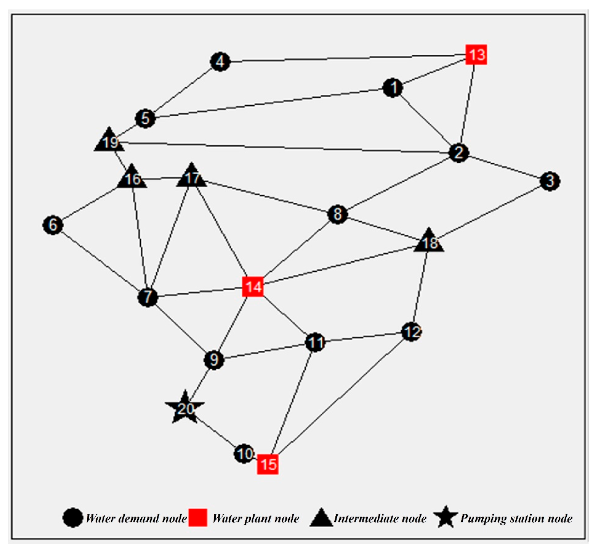
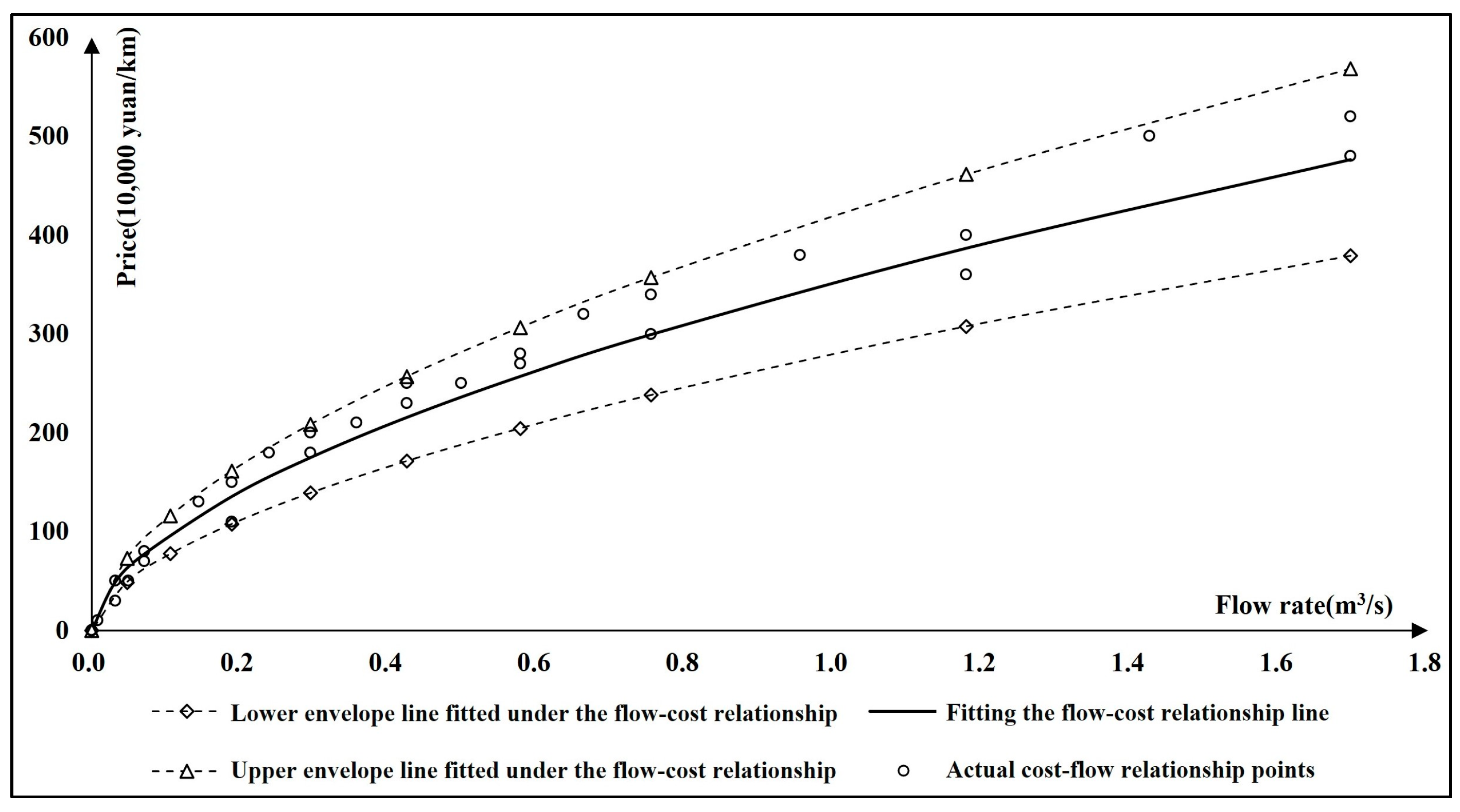
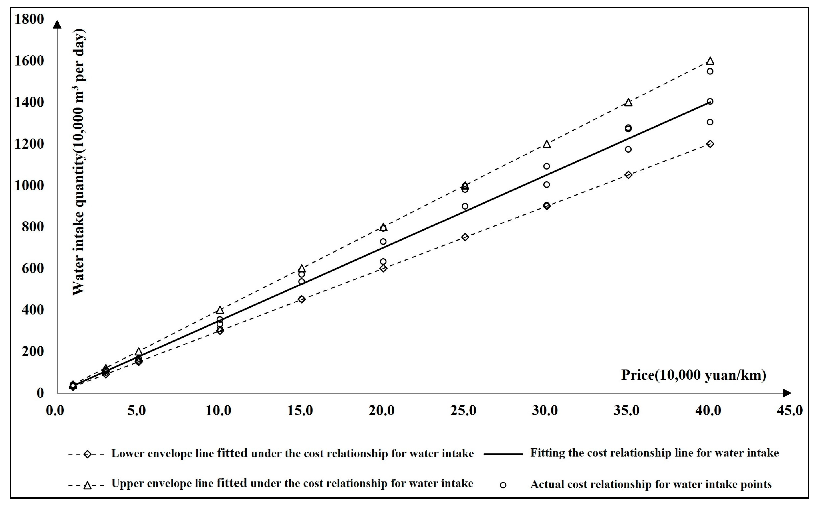
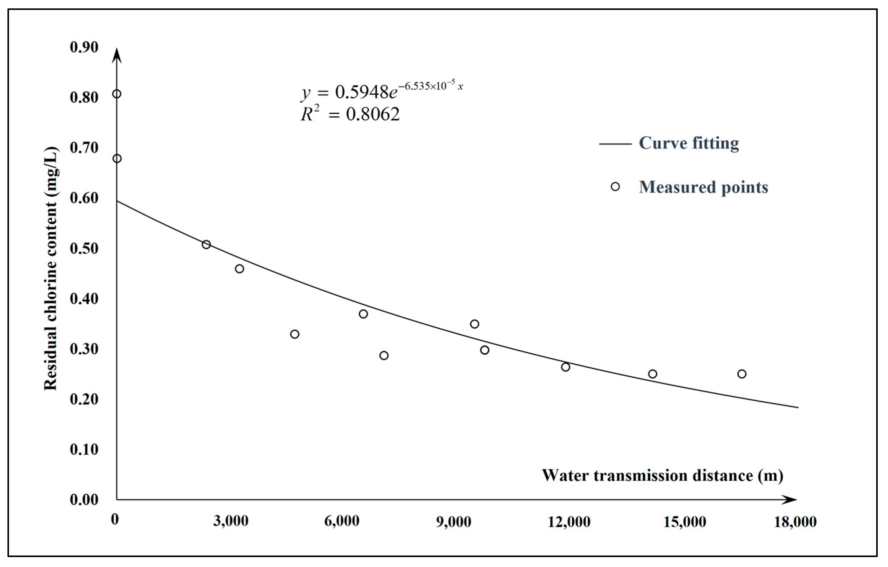
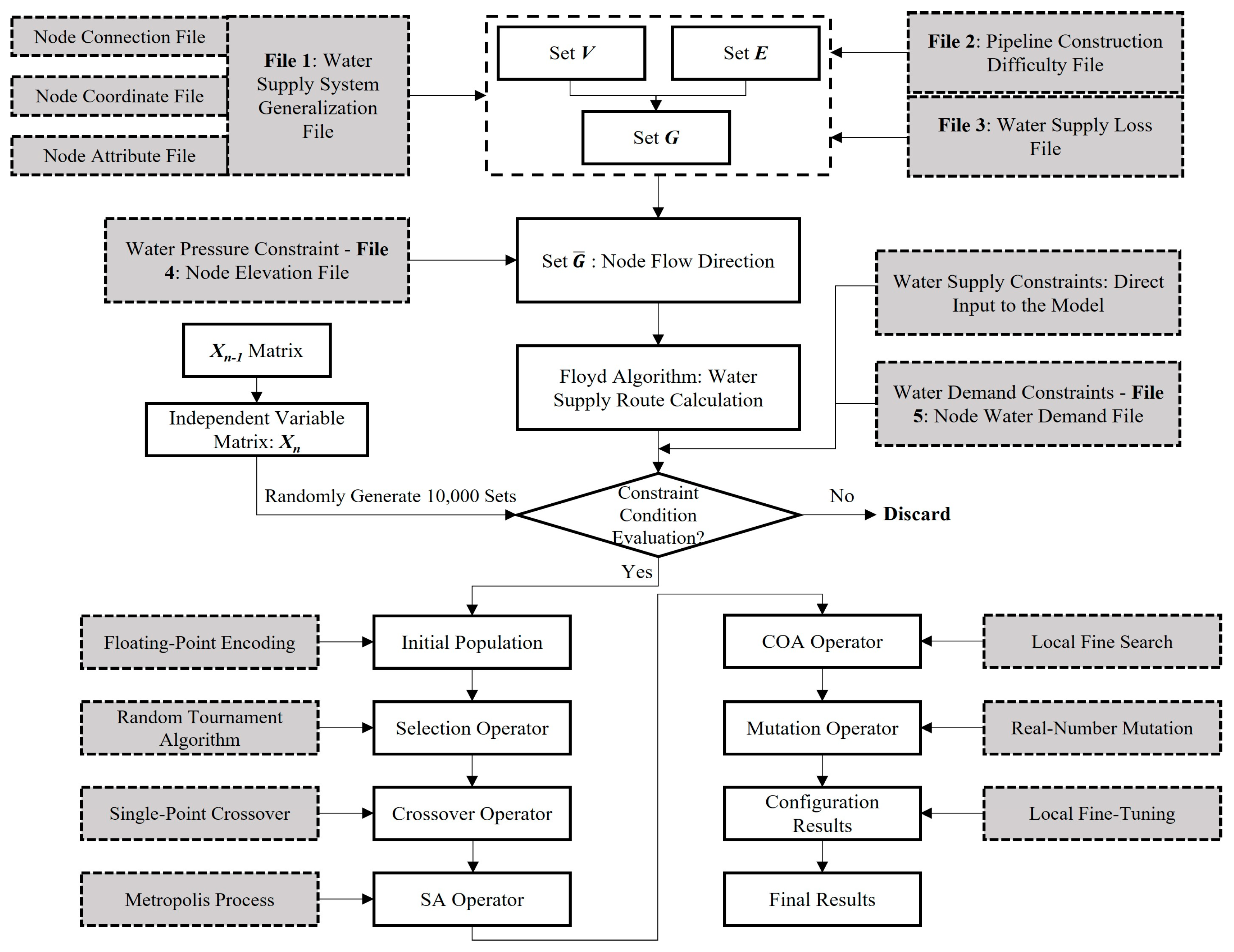
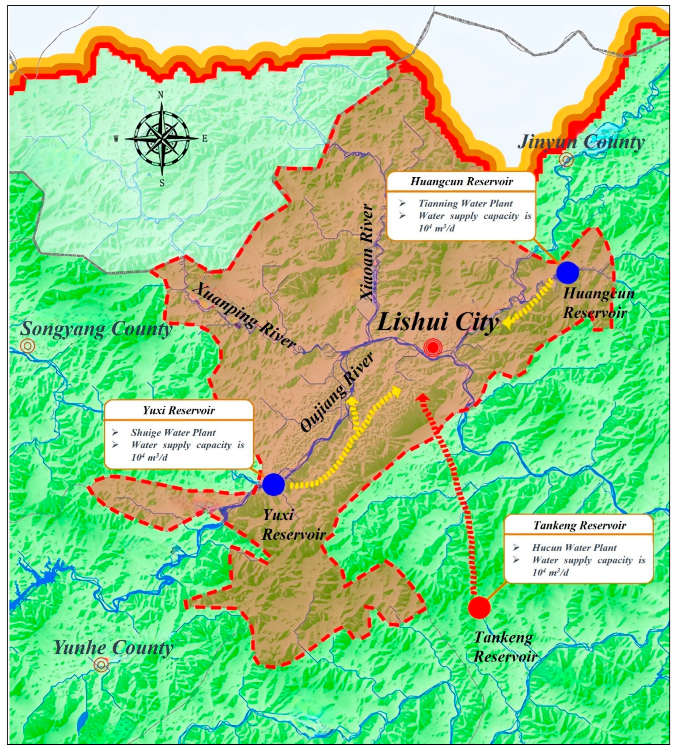
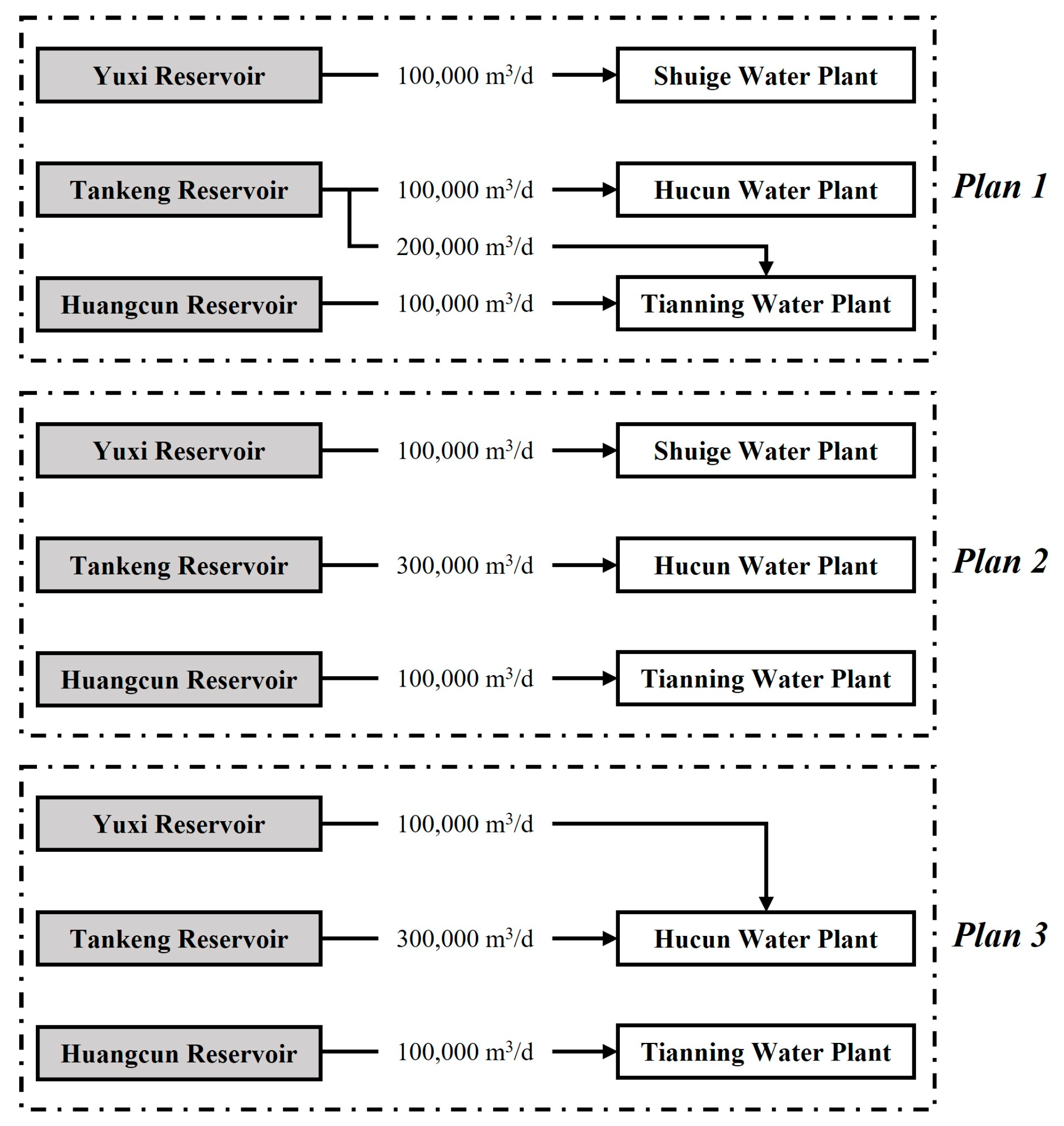

Disclaimer/Publisher’s Note: The statements, opinions and data contained in all publications are solely those of the individual author(s) and contributor(s) and not of MDPI and/or the editor(s). MDPI and/or the editor(s) disclaim responsibility for any injury to people or property resulting from any ideas, methods, instructions or products referred to in the content. |
© 2024 by the authors. Licensee MDPI, Basel, Switzerland. This article is an open access article distributed under the terms and conditions of the Creative Commons Attribution (CC BY) license (https://creativecommons.org/licenses/by/4.0/).