Study on the Impact of Climate Change on Water Cycle Processes in Cold Mountainous Areas—A Case Study of Water Towers in Northeastern China

Abstract

This study applied the fully coupled model WRF/WRF-Hydro to simulate land, air, and water cycles in the Changbai Mountain area (CMA) in Northeast China. This study evaluated the applicability of the coupled model in the region and analyzed the impact of regional climate change on the water cycle in the study area over the past half-century. The temperature in the Changbai Mountains increased significantly from 1975 to 2020. Precipitation, canopy water, and all types of evapotranspiration showed different increasing trends, whereas surface runoff showed a decreasing trend. The comparison revealed that precipitation, canopy water, canopy evaporation, and total evapotranspiration increased gradually in the low-latitude subbasins, whereas runoff decreased more rapidly. Runoff in the study area showed an annual double peak, which was due to snowmelt in spring and abundant precipitation in summer. Under the influence of climate change, the thawing time of frozen soil and snow cover in the study area will advance, leading to an increase in the spring runoff peak and earlier occurrence time. Our results provide a reference for the study of the water cycle process of the coupled model in cold mountainous areas and a scientific reference for the scientific response to climate change and the protection of regional water resource security.

1. Introduction

Over the past century, the global climate has changed significantly. The increase in temperature has led to the melting of ice sheets, an increase in sea level, and changes in the distribution and intensity of precipitation [1,2,3]. Precipitation and air temperature, as the main driving forces of land surface hydrological processes, significantly affect evapotranspiration and runoff processes [4,5]. Surface hydrology also affects the distribution of atmospheric water vapor and energy through evapotranspiration. Therefore, the water cycle is the most active and important link in land–air interactions. Land–air interactions are an important factor to be considered in the study of regional hydrological responses to climate change over long timescales.

Mountainous areas have complex topography, large vertical drops, and more active land, air, water, and energy transmission processes [6]. Mountainous areas generally receive more rainfall compared with plain areas and are often the “water towers” of a region owing to the dense network of rivers and groundwater channels formed in complex geological structures [7,8,9,10,11]. The CMA is an important “water tower” in northeast China. It is the source of the Tumen, Songhua, and Yalu River basins. It is in the core region of the global climate transcontinental zone in Northeast China [12]. The CMA has abundant rainfall, developed water systems, and a vast area of virgin forest with a great water conservation capacity. Regional water resources accounted for 78.6% of the total water resources in Jilin Province. Northeast China has been significantly affected by climate change over the past few decades [13]. The study of the response of the land–air–water cycle to climate change is of great significance for environmental management and protection in the Changbai Mountains, in addition to its importance for water resource utilization, ecological protection, and agricultural development in the lower reaches of the Changbaishan Mountains.

Studies have shown that mountain climates are cold, and the water cycle is complicated by the regulation of frozen soil and snow cover. This manifested in two ways. First, precipitation during the ice and snow seasons is stored in the form of snow cover, which is an important source of spring runoff. Secondly, the presence of frozen soil changes the way water is transported through the soil [14]. Pengfei Han’s study in the source area of the Yangtze River displayed that snowmelt water contributed 6.5–6.7% of the total annual runoff [15]. Based on model simulation results, Stewart calculated that snowfall in the western United States accounted for only 37% of the total precipitation, whereas snowmelt runoff accounted for 53% of the total runoff [16]. During snowmelt, the presence of frozen soil reduces the ability of water to infiltrate [17], such that snowmelt water can be converted into runoff more than rainfall [18]. Climate change significantly affects the regional water cycle, especially the freeze–thaw cycle. Few studies have been conducted to describe and simulate the effects of climate change on complex water cycling processes in mountainous areas under land–air interactions.

Due to the limitations of observational data, as well as the lack of station distribution coefficients and variables, model simulations are usually needed to describe the meteorological and hydrological changes in a watershed. Raster distributed hydrological models can fully consider the spatial differentiation of elevation, soil, vegetation cover, and land use and subsequently simulate the land surface water cycle process in a more refined manner [1,19,20,21]. However, distributed hydrological models are mostly driven by meteorological data and do not consider the interaction of energy and water between the atmosphere as well as the land surface. By coupling meteorological and hydrological models, the water cycle between the atmosphere and land surface can be realized, the response of the meteorological model to surface water vapor transport can be improved, and the description of hydrology in hydrological models can be improved [22,23]. Maxwell first attempted to combine hydrological models with Advanced Prediction Systems [24]. With the development and maturity of WRF, it has become increasingly used as well as the coupled atmospheric model. Chunling Tang evaluated the ability of WRF coupled with VIC to predict rainfall [25]. Sven Wagner developed a fully coupled model of the WRF and HMS for regional water balance simulations at regional and long-term scales [26]. Gochis developed the WRF-Hydro extension package based on Noah_LSM to achieve the coupling of the atmosphere, land surface, and groundwater [27].

In this study, the WRF/WRF-Hydro hydrological model was utilized to simulate regional water cycles. The research conducted by Qian et al. indicates that this model exhibits excellent performance in simulating water cycles in small and medium-sized catchments with high spatial resolution [28]. Simulations by Liu, using WRF-Hydro in a typical mountainous western river basin, display that the model accurately simulates the spatial variability as well as the evolution of runoff, evapotranspiration, soil temperature, and soil moisture [29]. Compared with offline WRF-Hydro, the fully coupled WRF/WRF-Hydro model can fully consider the mutual feedback of energy and water between the atmosphere and land surface and realize the closed simulation of the water cycle, thus improving the simulation effect of meteorological and hydrological elements. The comparative study showed that the simulation effect of the fully coupled WRF/WRF-Hydro on precipitation and runoff was better than that of the offline WRF-Hydro [30,31]. Compared with traditional hydrological models, fully coupled models have a wider application range and have been applied in the Mediterranean Sea region [27]. West Africa [32] and India [33]. However, few studies have been conducted on their application in cold mountainous regions.

In this study, the fully coupled WRF/WRF-Hydro Modeling System (WRF/WRF-Hydro Modeling System) was used to conduct a long-term quantitative hydrological simulation in the CMA, an important water tower in Northeast China. The main aims of this study are as follows: (1) to evaluate the applicability of the land–air coupling model in Northeast China. (2) Quantitative evaluation of the responses of meteorological and hydrological elements to climate change in the CMA. (3) The impacts of climate change on the regional water cycle and its mechanisms were analyzed. We aimed to reveal the response characteristics of land, air, and water cycles in important water source areas under the influence of climate change and provide a scientific reference for the security and efficient use of water resources in the Changbai Mountains in the future. And provide a basis for water resource management and environmental protection in mountain water towers. The research framework and methodology are summarized in Figure 1.

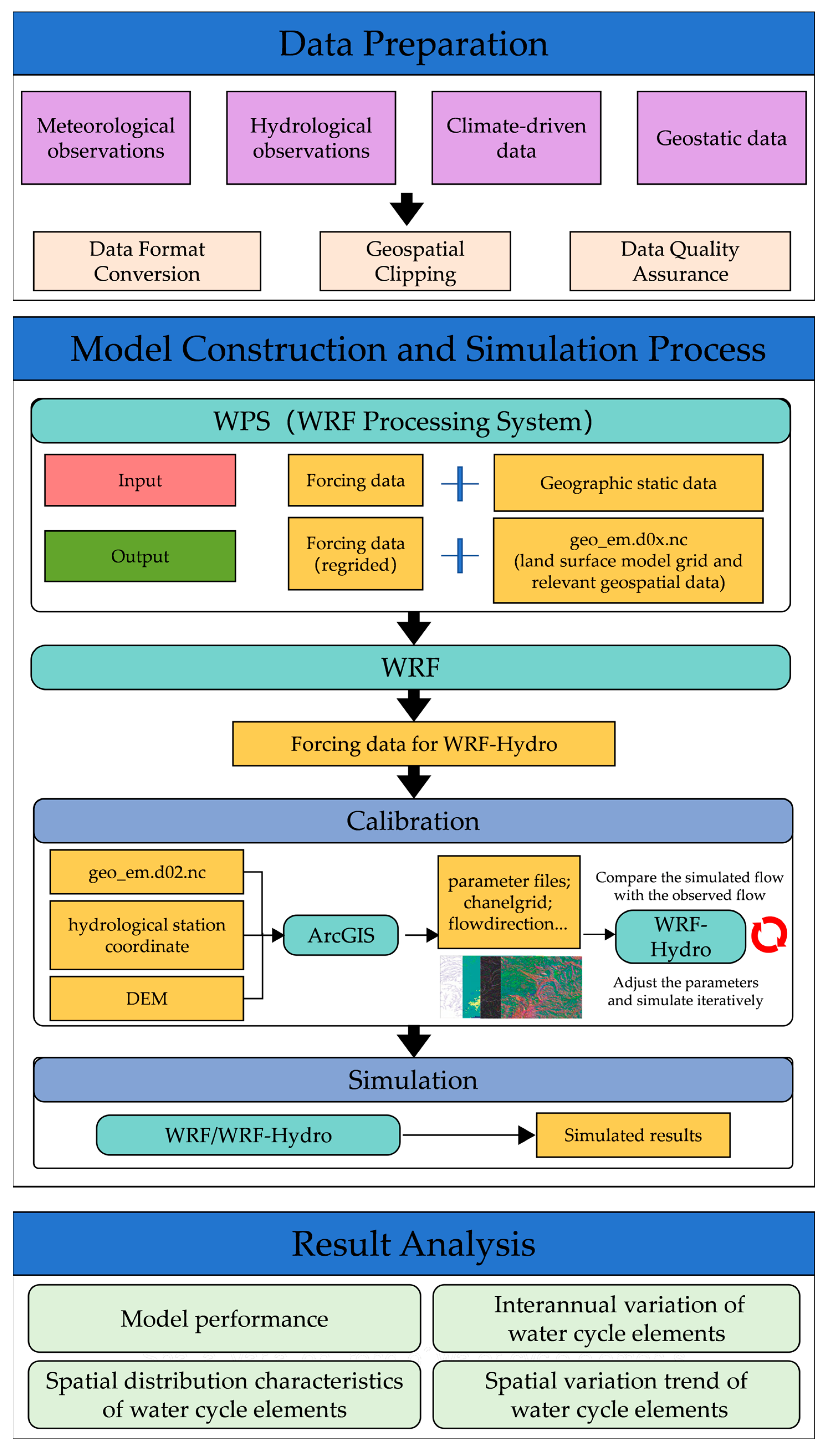
2. Materials and Methods

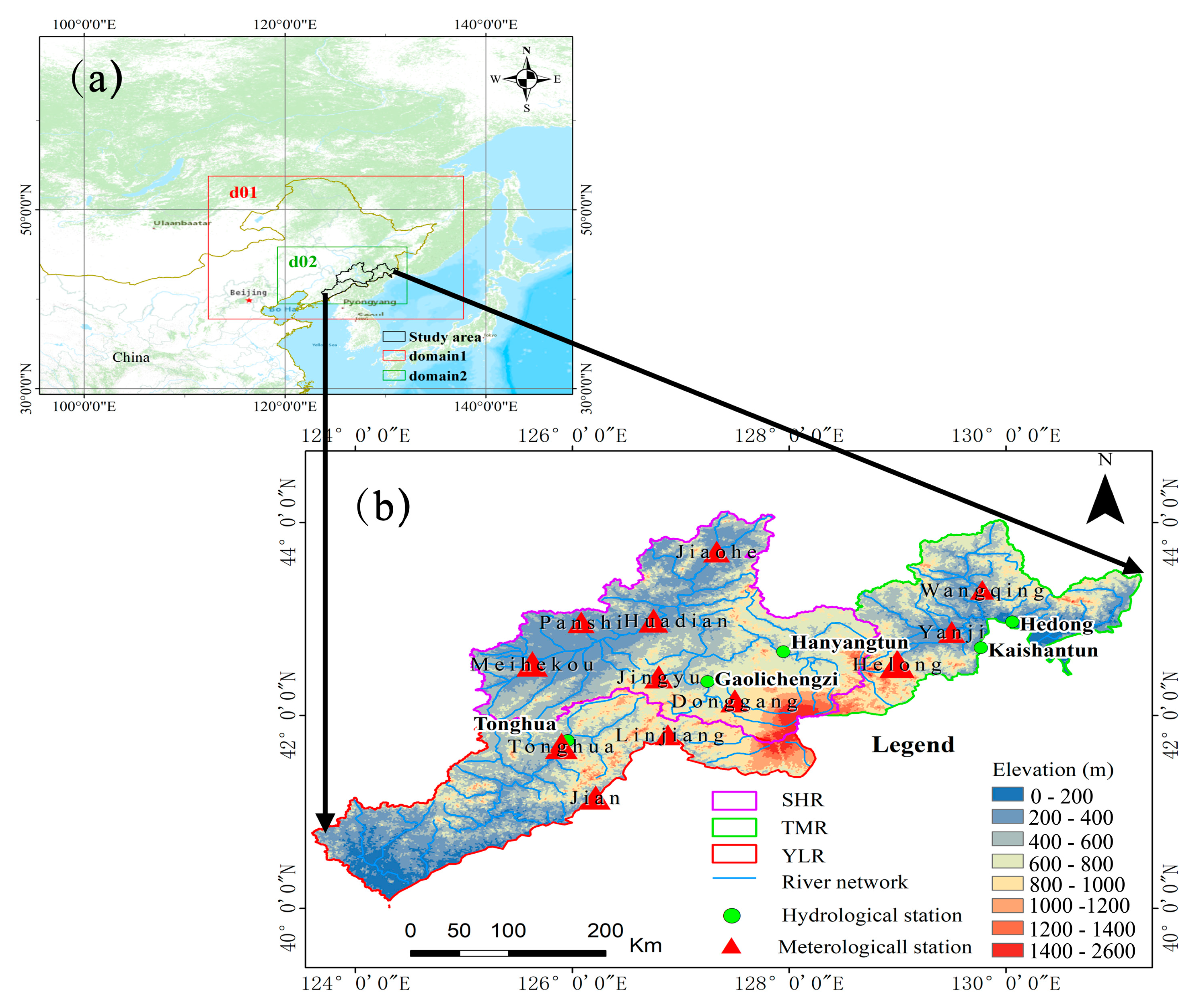
2.1. Study Area

The study area of this paper is the Changbai Mountain Area (CMA), which consists of the Songhua River Basin (SHR), the Tumen River Basin (TRB), and the Yalu River Basin (YRB), located at 123°36′–131°14′ E, 40°4′–44°6′ N, with a total area of about 96,000 km².

From the core area of Changbai Mountain, which is the source of the Songhua River, the Tumen River, and the Yalu River, the three sub-basins extend from south to north as the Tumen River basin, the Songhua River basin, and the Yalu River basin, as shown in Figure 2. The region experiences a temperate continental mountain climate characterized by cold winters, warm summers, and significant monsoon influence, with a high average altitude and long winter seasons. Based on observation data from meteorological stations, the study area has been significantly affected by climate change over the past decades, with the average temperature observed at the 12 stations showing a clear increasing trend (Figure 2b). The topography of this region is complex, and there are obvious differences in the vertical distribution of natural zones. Due to abundant precipitation and a developed water system, it is one of the most important water sources in Northeast China.

2.2. Data

The data from 12 meteorological stations used in the paper were obtained from the China Meteorological Data Network (http://data.cma.cn/) of the China Meteorological Administration. The daily runoff observations from five hydrological stations were selected for model rate and validation, and it was obtained from the Jilin Provincial Hydrological Bureau and the Songliao Water Resources Commission. The station names and geographical locations are also shown in Figure 2. Specific information on these hydrological and meteorological stations is given in

Table 1. Spatial location of meteorological and hydrological stations used in the study.

Type	Rivers	Site	Coordinates		Period of Record (Year)	Source
			Longitude	Latitude
Meterological Station	SHR	Jiaohe	127°33′ E	43°70′ N	1975–2020	China Meteorological Data Network (http://data.cma.cn/, accessed on 1 January 2023) of the China Meteorological Administration
		Huadian	126°76′ E	42°98′ N	1975–2020
		Jingyu	126°79′ E	42°40′ N	1975–2020
		Donggang	127°50′ E	42°15′ N	1975–2020
		Panshi	126°08′ E	42°96′ N	1975–2020
		Meihekou	125°66′ E	42°53′ N	1975–2020
	TMR	Wangqing	129°79′ E	43°30′ N	1975–2020
		Yanji	129°50′ E	42°87′ N	1975–2020
		Helong	129°00′ E	42°53′ N	1975–2020
	YLR	Linjiang	126°90′ E	41°80′ N	1975–2020
		Tonghua	125°92′ E	41°72′ N	1975–2020
		Jian	126°22′ E	41°15′ N	1975–2020
Hydrological Station	SHR	Hanyangtun	127°57′ E	42°39′ N	1975–2020	Jilin Provincial Hydrological Bureau and the Songliao Water Resources Commission
		Gaolichengzi	127°14′ E	42°21′ N	1975–2020
	TMR	Hedong	130°03′E	42°58′ N	1975,1980–2020
		Kaishantun	129°46′ E	42°42′ N	1975,1980–2020
	YLR	Tonghua	125°56′E	41°43′N	1980–2018

.

The forcing data are global, bias-corrected climate model output data from version of NCAR’s Community Earth System Model, which is developed to support WRF research. The data has a temporal resolution of 6 h and a spatial resolution of 0.9° × 1.25° [34]. The geographic static data used in the coupled model was obtained from the WRF users page (https://www2.mmm.ucar.edu/wrf/users/, accessed on 18 April 2023). High-resolution and high-quality terrain datasets, which should be processed for hydrologic connectivity, are the basis for WRF-Hydro to correctly define terrain parameters and terrain routing. The high-resolution DEM data used in this paper is obtained from the HydroSHEDS database (https://www.hydrosheds.org/, accessed on 15 July 2022) [35].

2.3. Models

In this study, the WRF/WRF-Hydro hydrological model was used to simulate the regional water cycle. The land surface hydrological model WRF-Hydro can simulate soil temperature, soil moisture (solid and liquid), snow cover, canopy water, energy fluxes, and water fluxes [36]. The WRF-Hydro can be run offline as a separate hydrological model or coupled with WRF to realize multi-scale meteorological and hydrological simulation and prediction. It has been widely used in scientific research and operational forecasting, and its main operational application example is the National Hydrological Model [37,38]. In scientific research, scholars have conducted many studies on the parameter sensitivity and uncertainty of WRF-Hydro. The results show that the model can obtain a good runoff simulation effect after parameter adjustment [28,39,40].

The fully coupled meteorological–hydrological model was constructed by WRF V4.2 and WRF-Hydro V5.1.2 and the computing platform provided by Beijing Super Cloud Computing Center (BsccCloud). Two nested domain schemes were used in the study, with a spatial resolution of 25 km for domain1 and 5 km for domain2 (Figure 2a). The physical process scheme of WRF was set in reference to the study of He Bohan [41] and Yu Entao [42] in Northeast China (

Table 2. Main WRF model physic options used for the study area.

Categories	Selected Option
Microphysics	WRF Singel-Moment 6class scheme (WSM6)
Cumulus parameterization	Kain-Fritsch
Planetary boundary layer	Yonsei University
Longwave radiation	Rapid Radiative Transfer Model (RRTM)
Shortwave radiation	Dudhia
Land surface model	Noah_MP

).

The simulation process is divided into three steps. Firstly, WRF is used to downscale the forcing data. Downscaled forcing data were used to drive the offline WRF-Hydro, and the hydrological parameters were calibrated by manual stepwise debugging. The calibrated parameters are shown in

Table 3. Calibrated parameters and description.

Prameter	Description	Units
REFKDT	A tunable parameter that significantly impacts surface infiltration and hence the partitioning of total runoff into surface and subsurface runoff.	unitless
RETDEPRTFAC	Multiplier on maximum retention depth before flow is routed as overland flow.	unitless
SLOPE	A coefficient that modifies the drainage out the bottom of the last soil layer.	unitless
OVROUGHRTFAC	A multiplier on Manning’s roughness for overland flow	unitless
MannN	Manning’s roughness coefficient.	s/m1/3
Zmax	A bucket model coefficient of the maximum storage in the bucket before “spilling” occurs.	unitless
SMCMAX	Maximum soil moisture content for each soil type.	m3/m3
LKSATFAC	Multiplier on saturated hydraulic conductivity in lateral flow direction.	m/s

.

In the third step, the fully coupled model was used, and the results were set to be output every 6 h, and each simulation time was 1 year. Especially, the December of the previous year was set as the warm-up time for the model. Figure 1 depicts the technology roadmap for this study, which includes the simulation process for the WRF/WRF-Hydro model.

2.4. Model Calibration

Distributed hydrological models provide amounts of adjustable hydrological parameters to support hydrological simulations in different regions, but the uncertainty of hydrological parameters leads to a huge workload for parameter calibration. Therefore, the important preliminary work is to pick out the parameters that have the greatest impact on the model results and have a clear mechanism of influence. Yucel [43] was the first to analyze the parameter sensitivity of the WRF-Hydro and proposed four important parameters. The highest priority should be given to the permeability coefficient (REFKDT) and the surface retention depth (REFKDEPRT), which can significantly control the amount of runoff. Subsequently, the surface roughness coefficient (OVROUGHRT) and the Manning coefficient (MannN) need to be considered, which can mainly control the shape and peak time of the flow curve. REFKDEPRT and OVROUGHRT are developed to be the two-dimensional parameters related to surface slope and soil type, and the new names were given, REFKDEPRTFAC and OVROUGHRTFAC, respectively. Liu Songnan found in the parameter study of WRF-Hydro that soil bottom drainage coefficient (SLOPE) and hydraulic conductivity (LKSATFAC) had a great influence on the simulation of soil moisture. In addition, the maximum soil moisture (SMCMAX) and the subsurface bucket model parameter (Zmax) were considered in this study. In the calibration process, four important parameters that significantly control the amount of water and the shape of the curve were first adjusted, and then the other parameters were gradually calibrated. The definition and initial values of each parameter can be found in Table 3 and the relevant technical manuals [43,44].

2.5. Static Method

The simulation performance of the coupled model was evaluated by three indicators, which are the correlation coefficient (CC), Nash efficiency coefficient (NSE), and RSR (the ratio of the root mean square error to the standard deviation), and they are defined by Equations (1)–(3). The CC represents the correlation coefficient between the simulated and observed values. The range of CC is between 0 and 1, and the closer to 1, the better the simulation. The value of NSE ranges from $-\infty$ to 1, and a value of 1 indicates that the simulation is completely consistent with the observed value. The higher NSE values indicate better model performance. RSR ranges from 0 to 1; the closer the value is to 0, the better the simulation.

$$CC={\displaystyle \frac{(n\sum \left(Q_{obs,i}{Q}_{sim,i}\right)-\sum \left(Q_{obs,i}{Q}_{sim,i}\right)}{\sqrt{n\sum {Q_{obs,i}}^2-{\left(\sum Q_{obs,i}\right)}^2}\sqrt{n\sum {Q_{sim,i}}^2-{\left(\sum Q_{sim,i}\right)}^2}}}$$

(1)

$$NSE=1-{\displaystyle \frac{\sum {\left(Q_{obs,i}-Q_{sim,i}\right)}^2}{\sum {\left(Q_{obs,i}-\overline{Q_{obs}}\right)}^2}}$$

(2)

$$RSR={\displaystyle \frac{\sqrt{\sum {(Q_{obs,i}-Q_{Sim,i})}^2}}{\sqrt{\sum {\left(Q_{obs,i}-\overline{Q_{obs}}\right)}^2}}}$$

(3)

where $Q_{obs,i}$ denotes the value of observed streamflow, $Q_{sim,i}$ denotes the value of simulated streamflow, $\overline{Q_{obs}}$ denotes the average value of observed streamflow, and n represents the length of streamflow series.

Pettitt test is a non-parametric mutation test method widely used in the field of meteorology and hydrology [45]. The original hypothesis $H_0$ is that there is no mutation point in time series. For time series $A_t\in \left[1,T\right]$, where T is the length of time series, and then $U_{t,T}$ is defined as follows:

$$U_{t,T}=U_{t-i,T}+{{\displaystyle \sum }}_{i=1}^{T}sgn\left(A_t-A_i\right)$$

(4)

$$sgn\left(A_t-A_i\right)=\left\{\begin{array}{c}+1,A_t>A\\ 0,A_t=A, i\in \left[1,t\right]\\ -1,A_t<A\end{array}\right.$$

(5)

Define the $K_t$, and when it satisfies Equation (6),

$$K_t=max\left|U_{t,T}\right| , 1\le i\le T$$

(6)

Then, t is the most likely mutation point, and the statistic p is introduced:

$$p=2exp\left[-{\displaystyle \frac{6K_t^2}{n^3+n^2}}\right]$$

(7)

If p < 0.05, the original hypothesis $H_0$ is rejected, and the mutation point is considered to be statistically significant.

3. Results

The performance of the model was evaluated using the observed streamflow data, and the results showed that the coupling model had a good long-term simulation effect in the study area. In this section, through the analysis of the high-resolution meteorological and hydrological data output by the model, the variation characteristics of water cycle elements in the study area were elaborated.

3.1. Model Performance

Five hydrological stations with relatively complete observation data in the study area were used for model performance evaluation, among which Tonghua station belongs to the YLR, Hanyangtun, and Gaolichengzi belong to the SHR, and Hedong and Kaishantun belong to the TMR (Figure 2b). Except for the Hedong station, the CC and NSE values of all stations exceeded 0.5 in the calibration period and the validation period and the RSR values were also very small, indicating that the overall simulation performance of the coupling model in the three sub-basins was good (

Table 4. The quantities of evaluation index on model performance.

Stations	Calibration Period (40%)			Validation Period (60%)
	CC	NSE	RSR	CC	NSE	RSR
Hanyangtun	0.84	0.67	0.57	0.78	0.57	0.65
Gaolichengzi	0.86	0.68	0.57	0.85	0.58	0.65
Tonghua	0.85	0.61	0.62	0.85	0.61	0.62
Kaishantun	0.78	0.57	0.68	0.80	0.60	0.64
Hedong	0.68	0.38	0.83	0.76	0.55	0.67

). Figure 3 shows the monthly streamflow simulated by the coupled model after calibration and the monthly streamflow data from the hydrological site observation.

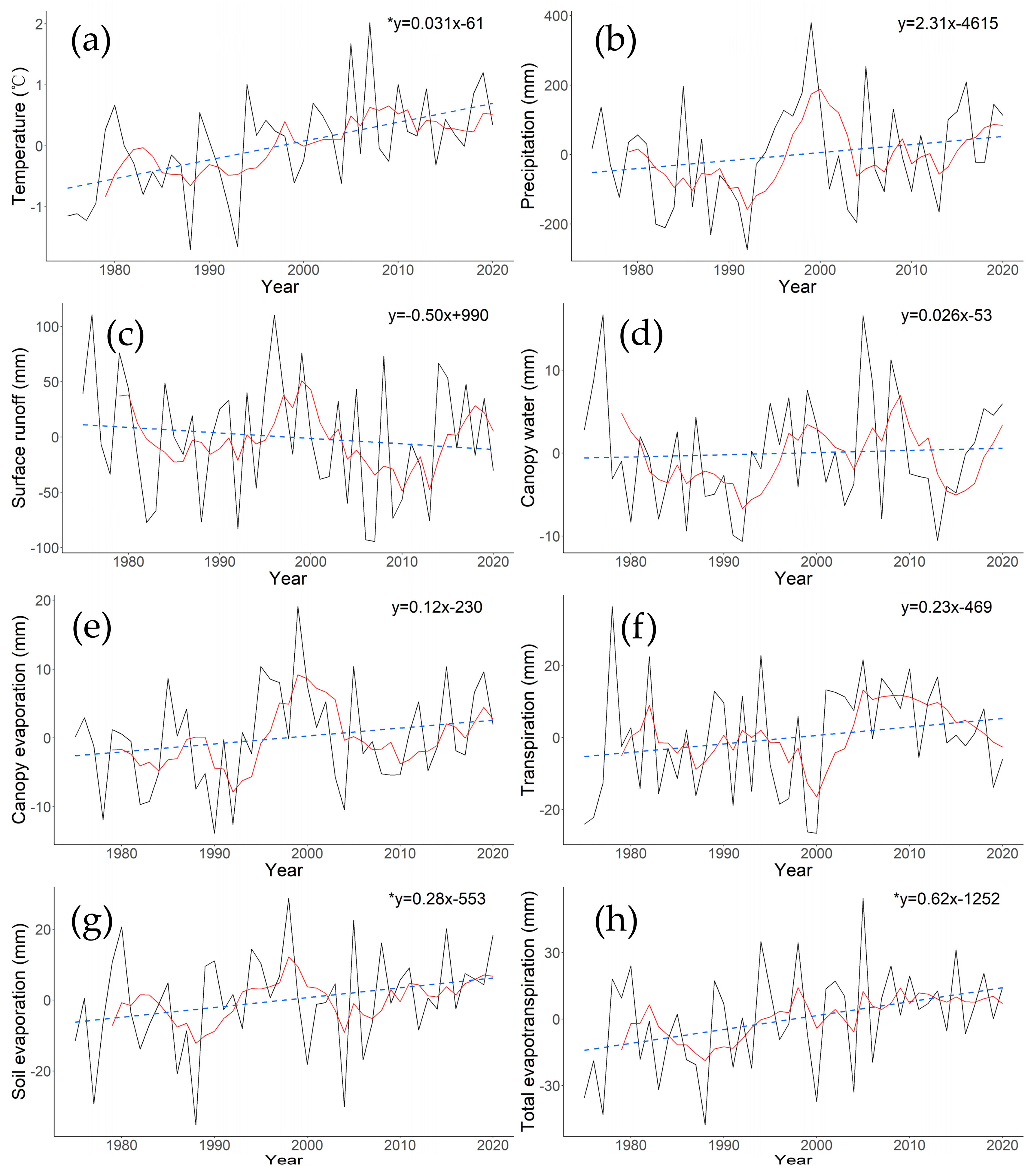
3.2. Interannual Variation of Water Cycle Elements

Further data analysis was conducted on the results of the long-time series water cycle elements output from the model, and we drew the regional annual mean distance level curves, 5-year sliding averages, and linear regression curves for each element (Figure 4). Based on the analysis, we reveal the characteristics of elemental changes in the study area over the last 50 years or so. The warming in the study area was very significant from 1975 to 2020, with a trend of 0.031 °C/a. With the increase in temperature, soil evaporation (0.28 mm/a), canopy evaporation (0.12 mm/a), plant transpiration (0.23 mm/a), and total evapotranspiration (0.63 mm/a) all showed an increasing trend. Precipitation in the study area also showed an increasing trend during the same period, with an increase rate of 2.31 mm/a while a decrease trend in surface runoff (−0.50 mm/a). The rising trend of canopy water (0.026 mm/a) is very weak. The mutation points of meteorological and hydrological elements were determined by the Pettitt method. The change ratio (Cr) is defined as the ratio of the post-mutation mean to the pre-mutation mean. The Tr1 and Tr2 represent the change trend before and after mutation, respectively, and the T represent the change trend from 1975 to 2020 (

Table 5. The abrupt change characteristics of meteorological and hydrological elements. The Cr is defined as the ratio of the post-mutation mean to the pre-mutation mean. The Tr₁ and Tr₂ represent the change trend before and after mutation, respectively, and the Tr represents the change trend from 1975 to 2020.

Elements	Mutational Point	Cr	Tr1	Tr2	Tr	p
Temperature (Temp)	2002	27.5%	0.036 °C/a	0.0068 °C/a	0.031 °C/a	0.001
Precipitation (Prcp)	2002	2.1%	4.59 mm/a	9.72 mm/a	2.31 mm/a	0.13
Surface runoff (Sfr)	1995	−1.2%	−2.00 mm/a	−1.01 mm/a	−0.50 mm/a	0.83
Canopy water (Cw)	2003	4.2%	−0.09 mm/a	−0.05 mm/a	0.026 mm/a	0.66
Canopy evaporation (Ecan)	2001	0.6%	0.38 mm/a	0.36 mm/a	0.12 mm/a	0.23
Transpiration (Etr)	1995	1.8%	0.44 mm/a	0.35 mm/a	0.23 mm/a	0.04
Soil evaporation (Es)	2007	2.7%	0.16 mm/a	0.37 mm/a	0.28 mm/a	0.16
Total evapotranspiration (Et)	2002	2.3%	0.80 mm/a	0.26 mm/a	0.63 mm/a	0.06

). Except for surface runoff, the other elements showed positive mean mutation. The change rate of temperature was the highest, reaching 27.5%. However, the rising trend of temperature slowed down after the mutation year. In addition, runoff, canopy water, canopy evaporation, plant transpiration, and total evapotranspiration all showed a lower change trend after the abrupt change point, while precipitation and soil evaporation showed a higher change trend after the abrupt change.

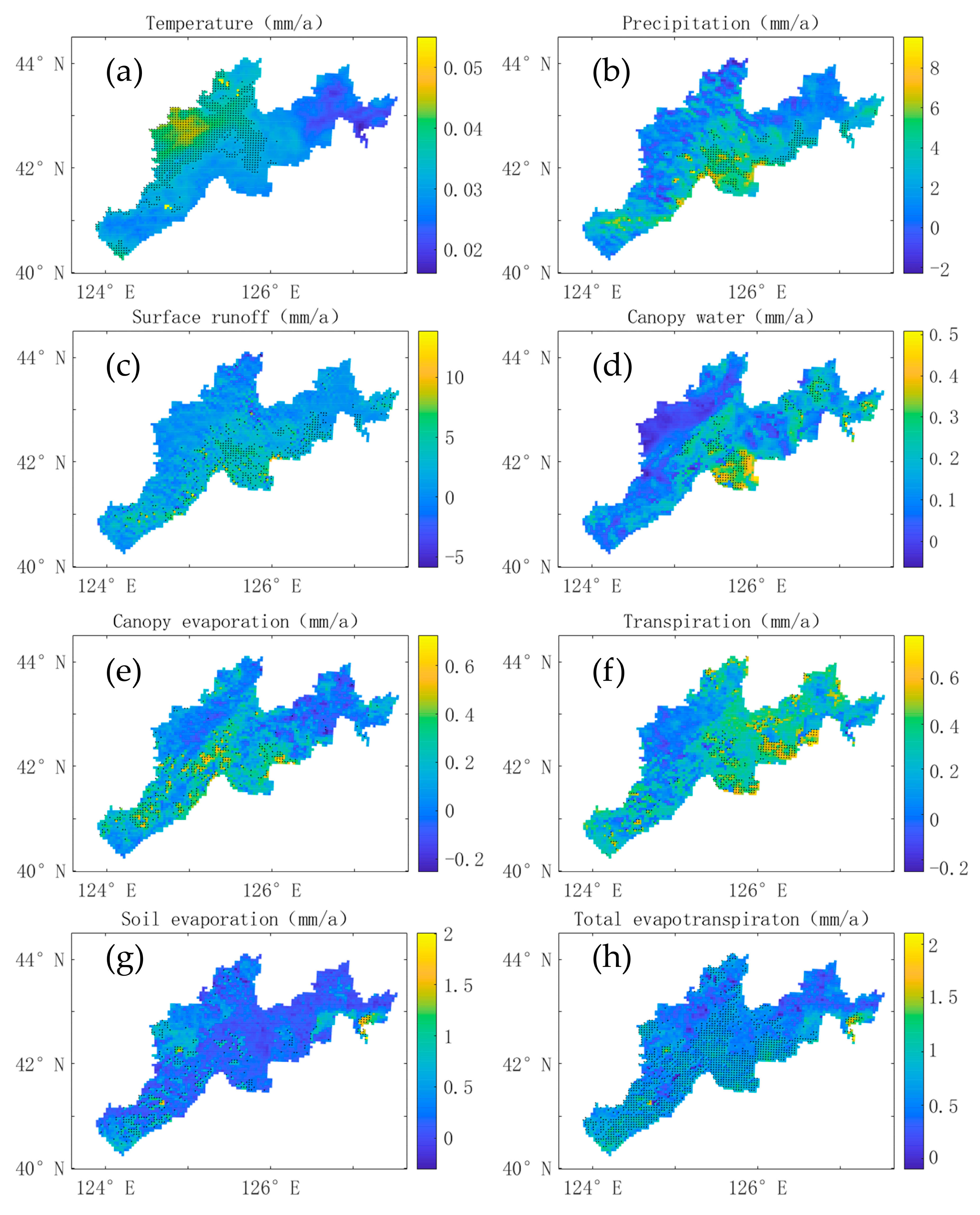
3.3. Spatial Distribution Characteristics of Water Cycle Elements

The fully coupled models are capable of multi-physical processes and multi-scale simulations; they have the advantage of being able to output high-resolution results of regional water cycle elements [46]. So, we can describe the spatial distribution and variation characteristics of regional water cycle elements more precisely and make up for the limitation of sparse distribution of observation stations. This section describes the spatial distribution characteristics of each element. The high-value areas of annual mean temperature in the study area are mainly located in the southern part of the YLR and the eastern part of the TMR, with lower mean temperatures in the core area of Changbai Mountain (Figure 5).

Precipitation is the most important pathway for atmospheric water transport to the land surface and determines the total water resources of the region. The spatial distribution of precipitation in the study area is not uniform, with high values in the core of Changbai Mountain and the SHR and relatively low precipitation in the TMR. The high value of canopy water is in the core area of Changbai Mountain and the central part of the CMA. Precipitation is an important recharge source for surface runoff, so the spatial distribution of surface runoff is more consistent with that of precipitation. However, under the effect of secondary distribution on the land surface, the divergent characteristics of surface runoff that are more obvious than that of precipitation, especially the high-value areas are more concentrated. Canopy evaporation and transpiration increased from northwest to southeast in the study area, while soil evaporation decreased from northwest to southeast. The total evapotranspiration decreased from west to east, with the lowest in the core area of Changbai Mountain and the TMR.

3.4. Spatial Variation Trend of Water Cycle Elements

Temperature is the most important feature of climate change, and it is also the most important factor affecting the regional water cycle [47]. For cold regions, the increase in temperature would affect the melting time and rate of snow cover and seasonally frozen soil [48]. From the perspective of the spatio-temporal variation trend (Figure 6), the area with an obvious temperature rise is mainly in the western part of the study area, and the temperature change in the north TMR is not obvious.

The regions with obvious increases in precipitation and temperature differed greatly, with the highest increasing trend of precipitation in the eastern part of the study area. The areas with a clear upward trend in canopy water are also mainly found in the eastern part of the study area, especially in the core area of Changbai Mountain. This is similar to precipitation, which may lead to a higher upward trend of canopy evaporation in the core area of Changbai Mountain. Plant transpiration showed an increasing trend except for the western part of the study area, while soil evaporation showed an increasing trend mainly in the western part and northeast corner of the study area. The spatial differences in the trends of total evapotranspiration are small but almost show an increasing trend in the whole region.

4. Discussions

4.1. Analysis of Model Uncertainties

The coupled model obtained better simulation results by describing the meteorological and land surface hydrological processes using well-established physical schemes. However, as the groundwater path and physical processes are unknown, the model uses a simple conceptual “Bucket” model to simulate the groundwater volume [49]. The model simplifies the water exchange process between groundwater, soil, and surface water through empirical equations; however, it does not have a real physical meaning [50]. The operation of the model is arithmetically demanding; therefore, the spatial resolution was compromised to achieve a long-term simulation. Lower spatial resolution tends to smooth the topography and is not conducive to runoff simulation; therefore, better results are achieved with a higher spatial resolution simulation [51].

4.2. The Hydrological Response to Climate Change

During 1975–2020, the average annual temperature in the study area showed a rising trend of 0.031 °C/a, which was slightly higher than that of China (1951–2021, 0.026 °C/a) and globally (1951–2021, 0.15 °C/a) in the last 50 years [12], indicating that the climate change in the study area was more significant. A hiatus in global warming occurred during 1998–2013 [52]. According to the abrupt change analysis, the rising temperature trend in the study area slowed after the abrupt change point (2002). From 1975 to 2020, precipitation showed an overall upward trend; however, its spatial distribution showed a significant regional agglomeration characteristic, and the increased rate of precipitation in the core area of Changbai Mountain and the middle and northeast of the YLR was significantly higher than that in the other areas. With a significant increase in precipitation, the risk of extreme precipitation in these regions has increased. For future water resource management and regional security, it is necessary to strengthen research on disaster prevention and emergency responses in these key regions [53,54]. While the precipitation in the study area displayed an upward trend, the surface runoff still showed a downward trend of 0.50 mm/a, which may be related to the increase of total evapotranspiration (0.62 mm/a). In addition, with population growth and social development, regional water intake continues to increase, which may lead to a decrease in regional runoff [55,56]. Compared with the influence of climate change, the contribution of human activities to changes in runoff could be higher [57]. The distribution of the three basins in the study area has obvious latitudinal differences, and the order from north to south is the TMR, SHR, and YLR.

A comparison of the variation trends of elements in the different basins showed that precipitation, canopy water, and total evapotranspiration increased slowly in the high-latitude basin (

Table 6. Interannual variation trend of water cycle elements in sub-basins.

Sub-Basin	Temp (°C/a)	Prcp (mm/a)	Sfr (mm/a)	Cw (mm/a)	Ecan (mm/a)	Etr (mm/a)	Es (mm/a)	Et (mm/a)
TMR	0.029	1.846	−1.285	−0.016	0.067	0.194	0.258	0.573
SHR	0.032	2.257	−0.217	0.054	0.097	0.271	0.283	0.597
YLR	0.031	3.297	0.094	0.056	0.212	0.243	0.279	0.734

). However, the increasing trend of surface runoff and precipitation in the YLR at the lowest latitude was higher than that in the other two basins, which may have also led to the highest rising trend of canopy water and total evapotranspiration in this basin. Although the Songhua River Basin is located in the middle, it has the most significant rising trend in temperature, which may be the reason for the rising trends of plant transpiration and soil evaporation being higher than those in the other two sub-basins [58,59].

4.3. The Impact on Water Cycle Process

The CMA is a seasonally frozen soil area, and its water resources mainly originate from precipitation. In spring (March–May), owing to low temperatures, the soil remained frozen in March (Figure 7). Precipitation was mostly in the form of snow, and evapotranspiration was low and dominated by soil evaporation (Figure 8).

From April to May, as the temperature increased, snow cover and thawing frozen soil gradually increased. Snowmelt water directly or indirectly supplements runoff through surface and lateral flows in the soil, which contributes to the peak runoff in spring. Feng Mingming’s isotope study in the core area of the Changbai Mountain showed that the contribution rate of snowmelt runoff to surface runoff in April–May was as high as 15.38% [60]. In summer (June–August), the frozen soil is completely thawed, and the surface water is replenished by abundant precipitation and groundwater, leading to the peak runoff in summer. Simultaneously, plants grow vigorously and cover the surface so that plant transpiration gradually exceeds soil evaporation and canopy evaporation gradually reaches its maximum value. In autumn (September–November), the soil was not frozen, and precipitation gradually decreased. With a decrease in temperature and vegetation, canopy evaporation and plant transpiration gradually decreased, and soil evaporation dominated the total evapotranspiration (Figure 8). In winter (December–February), snow is the main form of precipitation as rivers and soil gradually freeze, and evapotranspiration is low.

A significant increase in temperature leads to the arrival of snowmelt in advance [61]. From the soil state, the annual freezing time showed a downward trend when the initial surface soil freezing time was delayed, and the thawing time was advanced [62]. However, the second layer of frozen soil was less affected by the air temperature (Figure 9), and there was no obvious change in the thawing period.

After replenishing the surface soil moisture, snowmelt water could not penetrate deeper into the soil, thus forming more surface runoff [63]. This would lead to an increase in peak runoff in spring (Figure 10), and the peak would occur earlier. Zhou Xiaoyu’s study indicates that snowfall in Northeast China increased by 0.19 mm/a in the past few decades [13]. Chen Yongming’s study on snow cover in the CMA showed that the snowmelt rate in spring was significantly higher than that in the last century [12]. This means that there would be more runoff from snowmelt in spring, which would lead to a greater risk of spring flooding in the CMA.

5. Conclusions

The model was calibrated and verified using the observed runoff data. The CC and NSE values were almost all greater than 0.5, indicating that the performance of the model was good during the calibration and validation periods. Therefore, a fully coupled model can be applied to simulate the water cycle in cold mountainous regions.

The study area is very sensitive to climate change. From 1975 to 2020, temperature, precipitation, canopy water, canopy evaporation, plant transpiration, soil evaporation, and total evapotranspiration showed varying degrees of increasing trends. Precipitation, canopy water, canopy evaporation, and total evapotranspiration increased more slowly in the sub-basins located at lower latitudes. The surface runoff decreased more slowly in sub-basins located at lower latitudes and even displayed an upward trend. The CMA is a cold mountainous area with seasonally frozen soil. The form of precipitation and soil state result in different regional water cycle characteristics during different periods of the year. In one year, the regional runoff showed bimodal characteristics. As the temperature increased, the thawing of permafrost and snowmelt occurred earlier, leading to an earlier and larger spring runoff peak.

Against the backdrop of severe climate change and increasing human activity, a series of changes have occurred in the climate and underlying surfaces. The role of land–air interactions in the water cycle cannot be ignored. In long-term hydrological simulation and future scenario prediction studies, the land–air bidirectional coupling model is an effective research tool for long-term hydrological simulations and future scenario prediction studies.

References

1. Arnault, J.; Wei, J.; Rummler, T.; Fersch, B.; Zhang, Z.; Jung, G.; Wagner, S.; Kunstmann, H. A Joint Soil-vegetation-atmospheric Water Tagging Procedure with WRF-hydro: Implementation and Application to the Case of Precipitation Partitioning in the Upper Danube River Basin. Water Resour. Res. 2019, 55, 6217–6243. [Google Scholar] [CrossRef]
2. Special Report on Climate Change and Land—IPCC Site. Available online: https://www.ipcc.ch/srccl/ (accessed on 19 March 2025).
3. Intergovernmental Panel on Climate Change (IPCC). Climate Change 2021—The Physical Science Basis: Working Group I Contribution to the Sixth Assessment Report of the Intergovernmental Panel on Climate Change, 1st ed.; Cambridge University Press: Cambridge, UK, 2023; ISBN 978-1-009-15789-6. [Google Scholar]
4. Zhou, T. New Physical Science behind Climate Change: What Does IPCC AR6 Tell Us? Innovation 2021, 2, 100173. [Google Scholar] [CrossRef] [PubMed]
5. Climate and Hydrologic Ensembling Lead to Differing Streamflow and Sediment Yield Predictions/Climatic Change. Available online: https://link.springer.com/article/10.1007/s10584-021-03011-5 (accessed on 19 March 2025).
6. Stergiadi, M.; Di Marco, N.; Avesani, D.; Righetti, M.; Borga, M. Impact of Geology on Seasonal Hydrological Predictability in Alpine Regions by a Sensitivity Analysis Framework. Water 2020, 12, 2255. [Google Scholar] [CrossRef]
7. Nie, Y.; Pritchard, H.D.; Liu, Q.; Hennig, T.; Wang, W.; Wang, X.; Liu, S.; Nepal, S.; Samyn, D.; Hewitt, K.; et al. Glacial Change and Hydrological Implications in the Himalaya and Karakoram. Nat. Rev. Earth Environ. 2021, 2, 91–106. [Google Scholar] [CrossRef]
8. Viviroli, D.; Dürr, H.H.; Messerli, B.; Meybeck, M.; Weingartner, R. Mountains of the World, Water Towers for Humanity: Typology, Mapping, and Global Significance. Water Resour. Res. 2007, 43, 2006WR005653. [Google Scholar] [CrossRef]
9. Immerzeel, W.W.; Lutz, A.F.; Andrade, M.; Bahl, A.; Biemans, H.; Bolch, T.; Hyde, S.; Brumby, S.; Davies, B.J.; Elmore, A.C.; et al. Importance and Vulnerability of the World’s Water Towers. Nature 2020, 577, 364–369. [Google Scholar] [CrossRef]
10. Yagbasan, O.; Demir, V.; Yazicigil, H. Trend Analyses of Meteorological Variables and Lake Levels for Two Shallow Lakes in Central Turkey. Water 2020, 12, 414. [Google Scholar] [CrossRef]
11. Norbiato, D.; Borga, M.; Merz, R.; Blöschl, G.; Carton, A. Controls on Event Runoff Coefficients in the Eastern Italian Alps. J. Hydrol. 2009, 375, 312–325. [Google Scholar] [CrossRef]
12. Chen, Y.; Chang, Z.; Xu, S.; Qi, P.; Tang, X.; Song, Y.; Liu, D. Altitudinal Gradient Characteristics of Spatial and Temporal Variations of Snowpack in the Changbai Mountain and Their Response to Climate Change. Water 2021, 13, 3580. [Google Scholar] [CrossRef]
13. Zhou, Z.; Shi, H.; Fu, Q.; Li, T.; Gan, T.Y.; Liu, S.; Liu, K. Is the Cold Region in Northeast China Still Getting Warmer under Climate Change Impact? Atmos. Res. 2020, 237, 104864. [Google Scholar] [CrossRef]
14. Singh, P.; Wu, J.Q.; McCool, D.K.; Dun, S.; Lin, C.-H.; Morse, J.R. Winter Hydrologic and Erosion Processes in the U.S. Palouse Region: Field Experimentation and WEPP Simulation. Vadose Zone J. 2009, 8, 426–436. [Google Scholar] [CrossRef]
15. Han, P.; Long, D.; Han, Z.; Du, M.; Dai, L.; Hao, X. Improved Understanding of Snowmelt Runoff from the Headwaters of China’s Yangtze River Using Remotely Sensed Snow Products and Hydrological Modeling. Remote Sens. Environ. 2019, 224, 44–59. [Google Scholar] [CrossRef]
16. Stewart, I.T.; Cayan, D.R.; Dettinger, M.D. Changes in Snowmelt Runoff Timing in Western North America under a ‘business as Usual’ Climate Change Scenario. Clim. Change 2004, 62, 217–232. [Google Scholar] [CrossRef]
17. Demand, D.; Selker, J.S.; Weiler, M. Influences of Macropores on Infiltration into Seasonally Frozen Soil. Vadose Zone J. 2019, 18, 1–14. [Google Scholar] [CrossRef]
18. Bayard, D.; Stähli, M.; Parriaux, A.; Flühler, H. The Influence of Seasonally Frozen Soil on the Snowmelt Runoff at Two Alpine Sites in Southern Switzerland. J. Hydrol. 2005, 309, 66–84. [Google Scholar] [CrossRef]
19. Daniel, E.B. Watershed Modeling and Its Applications: A State-of-the-Art Review. Open Hydrol. J. 2011, 5, 26–50. [Google Scholar] [CrossRef]
20. Devia, G.K.; Ganasri, B.P.; Dwarakish, G.S. A Review on Hydrological Models. Aquat. Procedia 2015, 4, 1001–1007. [Google Scholar] [CrossRef]
21. Zeng, F.; Ma, M.-G.; Di, D.-R.; Shi, W.-Y. Separating the Impacts of Climate Change and Human Activities on Runoff: A Review of Method and Application. Water 2020, 12, 2201. [Google Scholar] [CrossRef]
22. Pietroniro, A.; Soulis, E.; Snelgrove, K.; Kouwen, N. A Framework for Coupling Atmospheric and Hydrological Models. In Proceedings of the International Symposium, Held During the Sixth IAHS Scientific Assembly, Maastricht, The Netherlands, 18–27 July 2001; pp. 27–34. [Google Scholar]
23. Majone, B.; Avesani, D.; Zulian, P.; Fiori, A.; Bellin, A. Analysis of High Streamflow Extremes in Climate Change Studies: How Do We Calibrate Hydrological Models? Hydrol. Earth Syst. Sci. 2022, 26, 3863–3883. [Google Scholar] [CrossRef]
24. Maxwell, R.M.; Chow, F.K.; Kollet, S.J. The Groundwater–Land-Surface–Atmosphere Connection: Soil Moisture Effects on the Atmospheric Boundary Layer in Fully-Coupled Simulations. Adv. Water Resour. 2007, 30, 2447–2466. [Google Scholar] [CrossRef]
25. Tang, C.; Dennis, R.L. How Reliable Is the Offline Linkage of Weather Research & Forecasting Model (WRF) and Variable Infiltration Capacity (VIC) Model? Glob. Planet. Change 2014, 116, 1–9. [Google Scholar] [CrossRef]
26. Wagner, S.; Fersch, B.; Yuan, F.; Yu, Z.; Kunstmann, H. Fully Coupled Atmospheric-hydrological Modeling at Regional and Long-term Scales: Development, Application, and Analysis of WRF-HMS. Water Resour. Res. 2016, 52, 3187–3211. [Google Scholar] [CrossRef]
27. Givati, A.; Gochis, D.; Rummler, T.; Kunstmann, H. Comparing One-Way and Two-Way Coupled Hydrometeorological Forecasting Systems for Flood Forecasting in the Mediterranean Region. Hydrology 2016, 3, 19. [Google Scholar] [CrossRef]
28. Xia, Q.; Fan, Y.; Zhang, H.; Jiang, C.; Wang, Y.; Hua, X.; Liu, D. A Review on the Development of Two-Way Coupled Atmospheric-Hydrological Models. Sustainability 2023, 15, 2803. [Google Scholar] [CrossRef]
29. Liu, Y.; Liu, J.; Li, C.; Yu, F.; Wang, W.; Qiu, Q. Parameter Sensitivity Analysis of the WRF-Hydro Modeling System for Streamflow Simulation: A Case Study in Semi-Humid and Semi-Arid Catchments of Northern China. Asia-Pac. J. Atmos. Sci. 2021, 57, 451–466. [Google Scholar] [CrossRef]
30. Wang, W.; Liu, J.; Li, C.; Liu, Y.; Yu, F.; Yu, E. An Evaluation Study of the Fully Coupled WRF/WRF-Hydro Modeling System for Simulation of Storm Events with Different Rainfall Evenness in Space and Time. Water 2020, 12, 1209. [Google Scholar] [CrossRef]
31. Wang, W.; Liu, J.; Xu, B.; Li, C.; Liu, Y.; Yu, F. A WRF/WRF-Hydro Coupling System with an Improved Structure for Rainfall-Runoff Simulation with Mixed Runoff Generation Mechanism. J. Hydrol. 2022, 612, 128049. [Google Scholar] [CrossRef]
32. Naabil, E.; Kouadio, K.; Lamptey, B.; Annor, T.; Chukwudi Achugbu, I. Tono Basin Climate Modeling, the Potential Advantage of Fully Coupled WRF/WRF-Hydro Modeling System. Model. Earth Syst. Environ. 2023, 9, 1669–1679. [Google Scholar] [CrossRef]
33. Sarkar, S.; Himesh, S. Evaluation of the Skill of a Fully-Coupled Atmospheric–Hydrological Model in Simulating Extreme Hydrometeorological Event: A Case Study over Cauvery River Catchment. Pure Appl. Geophys. 2021, 178, 1063–1086. [Google Scholar] [CrossRef]
34. Bruyere, C.; Monaghan, A.; Steinhoff, D.; Yates, D. Bias-Corrected CMIP5 CESM Data in WRF/MPAS Intermediate File Format; UCAR/NCAR: Boulder, CO, USA, 2015. [Google Scholar]
35. Lehner, B.; Verdin, K.; Jarvis, A. New Global Hydrography Derived from Spaceborne Elevation Data. EoS Trans. 2008, 89, 93–94. [Google Scholar] [CrossRef]
36. Ek, M.B.; Mitchell, K.E.; Lin, Y.; Rogers, E.; Grunmann, P.; Koren, V.; Gayno, G.; Tarpley, J.D. Implementation of Noah Land Surface Model Advances in the National Centers for Environmental Prediction Operational Mesoscale Eta Model. J. Geophys. Res. 2003, 108, 2002JD003296. [Google Scholar] [CrossRef]
37. Ensemble Data Assimilation for Flood Forecasting in Operational Settings: From Noah-MP to WRF-Hydro and the National Water Model|Semantic Scholar. Available online: https://www.semanticscholar.org/paper/Ensemble-Data-Assimilation-for-Flood-Forecasting-in-Zarekarizi/aed531e9ca2297e089daae98a31547fa67e86dde (accessed on 19 March 2025).
38. Ma, Y.; Chandrasekar, V.; Chen, H.; Cifelli, R. Quantifying the Potential of AQPI Gap-Filling Radar Network for Streamflow Simulation through a WRF-Hydro Experiment. J. Hydrometeorol. 2021, 22, 1869–1882. [Google Scholar] [CrossRef]
39. Yang, Y.; Yuan, H.; Yu, W. Uncertainties of 3D Soil Hydraulic Parameters in Streamflow Simulations Using a Distributed Hydrological Model System. J. Hydrol. 2018, 567, 12–24. [Google Scholar] [CrossRef]
40. Mane, D.; Chandrasekar, A. Evaluation of a Stand-Alone WRF-Hydro Modeling System Using Different Rainfall Forcing Data: Case Study over the Godavari River Basin, India. Pure Appl. Geophys. 2022, 179, 3807–3826. [Google Scholar] [CrossRef]
41. He, B.; Sun, Q.; Yu, E.; Wang, H.; Zhang, M.; Hua, W. Numerical simulation of the influence of topography of the Greater Khingan Mountains and Changbai Mountains on summer precipitation in northeast China. Clim. Environ. Stud. 2020, 25, 268–280. [Google Scholar]
42. Yu, E. High-Resolution Numerical Simulation of Seasonal Snowfall in Northeast China. Chin. Sci. Bull. 2013, 58, 690–698. [Google Scholar] [CrossRef]
43. Yucel, I.; Onen, A.; Yilmaz, K.K.; Gochis, D.J. Calibration and Evaluation of a Flood Forecasting System: Utility of Numerical Weather Prediction Model, Data Assimilation and Satellite-Based Rainfall. J. Hydrol. 2015, 523, 49–66. [Google Scholar] [CrossRef]
44. Niu, G.-Y.; Yang, Z.-L.; Mitchell, K.E.; Chen, F.; Ek, M.B.; Barlage, M.; Kumar, A.; Manning, K.; Niyogi, D.; Rosero, E.; et al. The community Noah land surface model with multiparameterization options (Noah-MP): 1. Model description and evaluation with local-scale measurements. J. Geophys. Res. Atmos. 2011, 116, D12109. [Google Scholar] [CrossRef]
45. Xue, Z.G.; Gochis, D.J.; Yu, W.; Keim, B.D.; Rohli, R.V.; Zang, Z.; Sampson, K.; Dugger, A.; Sathiaraj, D.; Ge, Q. Modeling Hydroclimatic Change in Southwest Louisiana Rivers. Water 2018, 10, 596. [Google Scholar] [CrossRef]
46. Eltahir, E.A.B.; Bras, R.L. Precipitation Recycling. Rev. Geophys. 1996, 34, 367–378. [Google Scholar] [CrossRef]
47. Baig, M.A.; Zaman, Q.; Baig, S.A.; Qasim, M.; Khalil, U.; Khan, S.A.; Ismail, M.; Muhammad, S.; Ali, S. Regression Analysis of Hydro-Meteorological Variables for Climate Change Prediction: A Case Study of Chitral Basin, Hindukush Region. Sci. Total Environ. 2021, 793, 148595. [Google Scholar] [CrossRef] [PubMed]
48. Wan, H.; Bian, J.; Zhang, H.; Li, Y. Assessment of Future Climate Change Impacts on Water-Heat-Salt Migration in Unsaturated Frozen Soil Using CoupModel. Front. Environ. Sci. Eng. 2021, 15, 10. [Google Scholar] [CrossRef]
49. Sofokleous, I.; Bruggeman, A.; Camera, C.; Eliades, M. Grid-Based Calibration of the WRF-Hydro with Noah-MP Model with Improved Groundwater and Transpiration Process Equations. J. Hydrol. 2023, 617, 128991. [Google Scholar] [CrossRef]
50. Mohammed, K.; Leconte, R.; Trudel, M. Impacts of Spatiotemporal Gaps in Satellite Soil Moisture Data on Hydrological Data Assimilation. Water 2023, 15, 321. [Google Scholar] [CrossRef]
51. Dixit, A.; Sahany, S.; Kanta Mishra, S. Modeling the Climate Change Impact on Hydroclimate Fluxes over the Beas Basin Using a High-Resolution Glacier-Atmosphere-Hydrology Coupled Setup. J. Hydrol. 2023, 627, 130219. [Google Scholar] [CrossRef]
52. Du, Q.; Zhang, M.; Wang, S.; Che, C.; Ma, R.; Ma, Z. Changes in Air Temperature over China in Response to the Recent Global Warming Hiatus. J. Geogr. Sci. 2019, 29, 496–516. [Google Scholar] [CrossRef]
53. Silva, D.G.; Silva Junior, J.R.D.D.; Souza, F.M.D.; Ramos, D.N.D.S.; Silva, A.R.; Santos, T.S.D.; Moreira, D.M. WRF-Hydro for Streamflow Simulation in the MATOPIBA Region within the Tocantins/Araguaia River Basin—Brazil: Implications for Water Resource Management. Water 2023, 15, 3902. [Google Scholar] [CrossRef]
54. Pasquier, U.; Vahmani, P.; Jones, A.D. Quantifying the City-Scale Impacts of Impervious Surfaces on Groundwater Recharge Potential: An Urban Application of WRF–Hydro. Water 2022, 14, 3143. [Google Scholar] [CrossRef]
55. Wang, J.; Liu, D.; Tian, S.; Ma, J.; Wang, L. Coupling Reconstruction of Atmospheric Hydrological Profile and Dry-up Risk Prediction in a Typical Lake Basin in Arid Area of China. Sci. Rep. 2022, 12, 6535. [Google Scholar] [CrossRef]
56. Towler, E.; Foks, S.S.; Dugger, A.L.; Dickinson, J.E.; Essaid, H.I.; Gochis, D.; Viger, R.J.; Zhang, Y. Benchmarking High-Resolution Hydrologic Model Performance of Long-Term Retrospective Streamflow Simulations in the Contiguous United States. Hydrol. Earth Syst. Sci. 2023, 27, 1809–1825. [Google Scholar] [CrossRef]
57. Zhang, Z.-Q.; Wu, Q.-B.; Hou, M.-T.; Tai, B.-W.; An, Y.-K. Permafrost Change in Northeast China in the 1950s–2010s. Adv. Clim. Change Res. 2021, 12, 18–28. [Google Scholar] [CrossRef]
58. Guo, S.; Tian, L.; Chen, S.; Liang, J.; Tian, J.; Cao, B.; Wang, X.; He, C. Analysis of Effects of Vegetation Cover and Elevation on Water Yield in an Alpine Basin of the Qilian Mountains in Northwest China by Integrating the WRF-Hydro and Budyko Framework. J. Hydrol. 2024, 629, 130580. [Google Scholar] [CrossRef]
59. Yin, D.; Xue, Z.G.; Bao, D.; RafieeiNasab, A.; Huang, Y.; Morales, M.; Warner, J.C. Understanding the Role of Initial Soil Moisture and Precipitation Magnitude in Flood Forecast Using a Hydrometeorological Modelling System. Hydrol. Process. 2022, 36, e14710. [Google Scholar] [CrossRef]
60. Feng, M.; Zhang, W.; Zhang, S.; Sun, Z.; Li, Y.; Huang, Y.; Wang, W.; Qi, P.; Zou, Y.; Jiang, M. The Role of Snowmelt Discharge to Runoff of an Alpine Watershed: Evidence from Water Stable Isotopes. J. Hydrol. 2022, 604, 127209. [Google Scholar] [CrossRef]
61. Mehboob, M.S.; Kim, Y. Impact of Climate Change on the Hydrological Projections over a Western Himalayan River Basin and the Associated Uncertainties. J. Hydrol. 2024, 628, 130460. [Google Scholar] [CrossRef]
62. Li, C.; Yu, G.; Wang, J.; Horton, D.E. Toward Improved Regional Hydrological Model Performance Using State-of-the-science Data-informed Soil Parameters. Water Resour. Res. 2023, 59, e2023WR034431. [Google Scholar] [CrossRef]
63. Li, X.; He, H.S.; Li, N.; Yu, H.; Zong, S.; Wu, Z.; Du, H. Season-Dependent Climate Sensitivity of the Surface Runoff of Major Rivers in Changbai Mountain. J. Hydrol. 2024, 643, 131936. [Google Scholar] [CrossRef]
Figure 1. Flowchart of the research methodology.
Water 17 00969 g001
Figure 2. Study site location. (a) Study location and model nesting area settings. (b) The location of the observation station and the size of the mark of the meteorological station represent the magnitude of the rising temperature.
Water 17 00969 g002
Figure 3. Comparison of simulated and observed flows at hydrological sites from 1975 to 2020. Because some observations are missing, they are not plotted in the figure. (a) Hanyangtun hydrological station; (b) Gaolichengzi hydrological station; (c) Tonghua hydrological station; (d) Kaishantun hydrological station; (e) Hedong hydrological station.
Water 17 00969 g003
Figure 4. The annual variation trend characteristic of each element, the black line is the anomaly curve, the red line is the five-year moving average, and the blue dashed line is the regression curve. The * marks that the variation trend is significant at the 95% confidence level. Subfigures represent different elements: (a) temperature; (b) precipitation; (c) surface runoff; (d) canopy water; (e) canopy evaporation; (f) transpiration; (g) soil evaporation; (h) total evapotranspiration.
Water 17 00969 g004
Figure 5. Spatial distribution of each element, and the value is the mean of multi-year in 1975–2020. Subfigures represent different elements: (a) temperature; (b) precipitation; (c) surface runoff; (d) canopy water; (e) canopy evaporation; (f) transpiration; (g) soil evaporation; (h) total evapotranspiration.
Water 17 00969 g005
Figure 6. Spatio-temporal variation trend of each element. Trends for each grid were calculated from annual values for the period 1975–2020, and the trend of the grid, which is marked with a dot, is significant at the 95% confidence level. Subfigures represent different elements: (a) temperature; (b) precipitation; (c) surface runoff; (d) canopy water; (e) canopy evaporation; (f) transpiration; (g) soil evaporation; (h) total evapotranspiration.
Water 17 00969 g006
Figure 7. The soil temperature and humidity changes in each layer. The soil is divided into four layers, including (a) the first layer: 0–10 cm; (b) the second layer: 10–40 cm; (c) the third layer: 40–100 cm; (d) the fourth layer: 100–200 cm.
Water 17 00969 g007
Figure 8. Annual variation of water cycle elements includes (a) temperature and evapotranspiration, (b) precipitation and runoff.
Water 17 00969 g008
Figure 9. Interannual variation trend of soil freeze–thaw condition: (a,b) show the changes in the first layer, (c,d) show the changes in the second layer.
Water 17 00969 g009
Figure 10. Trend of surface runoff peak in spring.
Water 17 00969 g010