Abstract
The functional relationship between soil permittivity and soil water content serves as the theoretical foundation for electromagnetic wave-based techniques used to determine soil moisture levels. However, the response of permittivity to changes in soil water content varies significantly across different soil types. Current models that utilize soil permittivity to estimate soil water content are often based on empirical statistical relationships specific to particular soil types. Moreover, existing physical models are hindered by an excessive number of parameters, which can be difficult to measure or calculate. This study introduces a universal model, termed the Soil Refractive Index (SRI) model, to describe the relationship between soil permittivity and soil water content. The SRI model is derived from the propagation velocity of electromagnetic waves in various soil components and the functional relationship between electromagnetic wave velocity and relative permittivity. The SRI model expresses soil water content as a linear function of the square root of the relative permittivity for any soil type with the slope and intercept as the two undetermined parameters. The slope is primarily influenced by the relative permittivity of soil water, while the intercept is mainly affected by both the slope and the soil porosity. The applicability of the SRI model is validated through tested soil samples and comparison with previously published empirical statistical models. For dielectric lossless soil, the theoretical value of the slope is calculated to be 0.126. The intercept varies across different soil types and increases linearly with soil porosity. The SRI model provides a theoretical basis for calculating soil water content using permittivity across various soil types.
1. Introduction
Soil water content (θ) is a critical parameter in agriculture, hydrology, and environmental monitoring. The accurate measurement of θ is essential for optimizing irrigation, managing water resources, and understanding soil–plant–atmosphere interactions. Among the various methods for determining θ, electromagnetic wave-based techniques have gained widespread adoption due to their nondestructive nature and efficiency. These techniques rely on the relationship between soil water content and soil relative permittivity (ε), which describes how easily a material can be polarized under an electric field. The large difference in relative permittivity among water (≈80), air (≈1), and soil solids (3–10) makes ε a sensitive indicator of θ.
Electromagnetic wave-based instruments, such as Ground Penetrating Radar (GPR) [1,2,3,4], Time Domain Reflectometry (TDR) [5,6], Frequency Domain Reflectometry (FDR) [7], and capacitance sensors [8,9], utilize the θ-ε relationship to estimate soil water content. Even in active microwave remote sensing, the retrieval of surface soil moisture is based on the contrast in ε between dry soil and water [10]. Despite the widespread use of these techniques, the accuracy of θ estimation depends heavily on the reliability of the θ-ε relationship, which varies significantly across soil types. Therefore, establishing a robust and universal θ-ε model is crucial for improving the precision of soil water content measurements.
Existing models for describing the θ-ε relationship can be broadly categorized into empirical and physical models. Empirical models, such as the widely used Topp equation [11], employ polynomial or linear fits to experimental data. While these models are simple and effective for specific soil types, they lack generalizability. For instance, Roth et al. [12] demonstrated that the Topp equation significantly underestimates θ for certain mineral soils. Moreover, empirical models are limited by their dependence on specific datasets and cannot be extrapolated beyond the tested range of conditions, prompting other researchers to develop alternative equations based on their experimental data [13,14]. These limitations highlight the need for models that can adapt to diverse soil types and conditions.
Physical models, on the other hand, treat soil as a multiphase mixture of dielectric components and provide a theoretical foundation for the θ-ε relationship. Examples include the composite discrete model [15,16,17], composite sphere model [18], composite confocal model [19] and power law dielectric mixing model [2,20,21]. While physical models offer a more universal framework, their practical application is hindered by the complexity of parameter determination. For instance, the power law dielectric mixing model requires parameters such as soil porosity, soil matrix permittivity, and a geometric factor, which are difficult to measure or estimate accurately [20,22,23,24,25,26]. As a result, physical models are often simplified into semi-empirical forms, limiting their utility for broad application.
To address these challenges, this study proposes a novel Soil Refractive Index (SRI) model, which is derived from the propagation velocity of electromagnetic waves in soil and the relationship between wave velocity and relative permittivity. The SRI model provides a general form of the θ-ε relationship applicable to any soil type with parameters that are physically interpretable and easier to determine. The validity of the SRI model is demonstrated through laboratory experiments on three soil types and comparisons with existing models. Additionally, the specific values and calculation methods for model parameters are provided, offering a practical tool for accurate soil water content estimation across diverse soil conditions.
2. Materials and Methods
2.1. Basic Theory
The relative permittivity (ε) of soil is generally complex and can be expressed as
where ε is the relative complex permittivity, is the real component, is the imaginary component, and . The real component () is related to the energy stored in the soil as molecules align within an alternating electric field, while the imaginary component () represents energy losses in the soil under the same conditions.
The imaginary component is related to two basic processes, electrical conduction and dielectric losses, and can be expressed as
where is the relative permittivity due to dielectric losses caused by polar molecules (e.g., water), is the electrical conductivity at zero frequency (S/m), also known as direct current conductivity, is the electromagnetic frequency, and is the permittivity of free space (8.854 × 10⁻¹² F/m).
The magnitude of the imaginary component relative to the real component is quantified by the loss tangent (), which reflects the impact of on soil water content calculations. It is defined as
In a three-phase soil mixture, the propagation speeds of electromagnetic waves in soil, water, and the soil matrix are denoted as , and , respectively. The volumetric water content and soil porosity are represented by and , respectively. The total propagation time within a soil sample can be considered as the sum of travel times through each component, leading to the following equation:
where is the electromagnetic wave velocity in air (≈0.3 m/ns). Rearranging Equation (4) yields
The electromagnetic wave speed in a medium is related to its relative permittivity as follows:
where is the electromagnetic wave speed in any medium, is the real component of relative permittivity, and is the relative magnetic permeability. For non-magnetic media (most soils are non-magnetic), . The term related to in Equation (6) is defined as the Deceleration Factor (DF) of the electromagnetic wave, which is denoted as :
The DF has the maximum value of 1 if , such as for free space, and the minimum value of 0 if , such as for a conductor.
Combining Equations (5)–(7), we obtain
where , and are the Deceleration Factors (DFs) of the soil, soil water and soil matrix, and , and are the real components of complex permittivity for the soil, soil water and soil matrix.
In soil, water is a typical polar molecule, while air and most soil particles are non-polar media. When the electromagnetic wave frequency is much lower than the relaxation frequency of water molecules (17.1 GHz), the imaginary component of relative permittivity () can be neglected compared to the real component in moist soil and water. This condition applies to most soil water content detection technologies, such as Hydra GO, TDR, GPR, FDR, and TDT [1,8,27,28]. For dielectric lossless soils (low clay content and salinity, ), , and . Thus, Equation (8) simplifies to
To generalize the relationship between soil water content and permittivity for all soil types, we rewrite Equations (8) and (9) as
where
and
In Equation (10), the relationship between and is expressed as a linear function between and , where is the slope and is the intercept. For dielectric lossless soils, is determined solely by the relative permittivity of soil water (), while depends on , soil porosity (), and the relative permittivity of the soil matrix (). For dielectric loss soils (e.g., clay-rich or high-salinity soils), and are also influenced by the Deceleration Factor (DF), which is determined by (Equation (7)). Since increases with water content and varies significantly with soil type [29], it is challenging to determine the specific values of DF for different soil components. Generally, in dielectric loss soils, and , as dielectric losses in moist soil are primarily contributed by soil water. Consequently, the slope parameter () for dielectric loss soils is typically lower than that for dielectric lossless soils under the same conditions.
Comparing Equations (8) and (9), it is evident that a linear relationship between and exists for all soil types regardless of dielectric losses. Since is equivalent to the refractive index of an electromagnetic wave passing from air to soil, we refer to Equation (10) as the Soil Refractive Index (SRI) model for soil water content estimation.
2.2. Laboratory Experiments
Three distinct soil types—organic soil (OS), humus soil (HS), and sandy soil (SS)—were collected from different geographical locations to ensure a representative range of soil properties. Both OS and HS were collected in the Great Khingan region of northeast China. OS was excavated from the loose layer of vegetative roots and dead leaves. This area is characterized by abundant moss and blueberry growth, contributing to the high organic matter content of the soil. HS was obtained from the highly decomposed black humus layer of riparian beach land, where inverted tallgrass meadows are prevalent. The high decomposition level of organic materials in this layer makes HS rich in organic matter. SS was collected from a wind-formed sandy area on an ancient riverbed in Wudaoliang, Qinghai–Tibet Plateau. SS represents a typical mineral soil with low organic matter content and high sand fraction.
After collection, the soil samples were transported to the laboratory for processing. The samples were oven-dried at 105 °C for 48 h to remove moisture. The dried soils were manually ground and passed through a 2 mm sieve to eliminate larger particles such as roots, leaves, and gravel. This step ensured that the prepared soil samples were homogeneous and suitable for subsequent testing.
Key soil parameters, including organic matter content (OM), particle density (PD), bulk density (ρ), and soil texture, were analyzed by a specialized soil testing laboratory at The Second Geological and Mineral Exploration Institute of Gansu Provincial Bureau of Geology and Mineral Exploration and Development. Due to the high organic matter content in OS and HS, the organic matter content (OM) of our tested soils was measured by direct cauterization in a muffle furnace at 600 °C, and the results were expressed as weight percentage. Particle density (PD) was measured using a pycnometer (specific gravity bottle), which provides insights into the intrinsic density of soil particles, excluding pore spaces. ρ was measured by weighing oven-dried (105 °C) soil samples made with a ring sampler. Together with particle density (PD), bulk density (ρ) was used to calculate porosity, which is a unitless ratio representing the volume of pore space divided by the total volume of the soil. The proportions of sand (0.075–2 mm), silt (0.005–0.075 mm), and clay (<0.005 mm) were determined using a laser particle size analyzer (Winner 2309) with results expressed as volume percentages.
The tested parameters for each soil type are summarized in Table 1. These include OM, PD, ρ, and the proportions of sand, silt, and clay, which were the averaged results of three duplicate samples. The data highlight the distinct characteristics of OS, HS, and SS, providing a comprehensive basis for validating the SRI model across diverse soil types.

Table 1.
Laboratory tested soil characteristic parameters.
The tested parameters for each soil type are summarized in Table 1, including OM, PD, ρ, and the proportions of sand, silt, and clay. These values represent the averaged results with maximum error ranges derived from three duplicate samples. The data highlight the distinct characteristics of OS, HS, and SS, providing a robust basis for validating the SRI model across diverse soil types.
The relative complex permittivity () and loss tangent () were measured using the Hydra GO device (Stevens Water Monitoring Systems, Inc., Portland, OR, USA), which employs Hydra Probe Soil Sensor technology. The device generates a 50 MHz electromagnetic wave transmitted via planar waveguides to its tines, providing temperature-corrected real () and imaginary () components of relative permittivity. The relative complex permittivity measurement error for each soil sample was within 0.1 for repeated measurements.
Deionized water was incrementally added to oven-dried soil samples and manually mixed to ensure uniform moisture distribution. After each water addition, the relative complex permittivity () and volumetric water content were measured to establish the relationship between soil moisture and dielectric properties. For humus soil (HS) and sandy soil (SS), two replicated soil samples were manually compacted into a 1200 mL round metal container (height: 8.5 cm, diameter: 13.4 cm). The compaction process ensured consistent soil density across replicates. The Hydra GO device was inserted into the center of the container to measure permittivity. Following the permittivity measurements, three ring knife samples were collected from each replicate to determine the soil water content and bulk density. The max error of soil water content measured by three ring knife samples was within 0.01 m3/m3, which demonstrates that our prepared soil samples were homogeneous. For organic soil (OS), three replicated oven-dried soil samples of the same weight were compacted into 2000 mL beakers. Due to the high fibrous content of OS, traditional ring knife sampling was impractical. Instead, the soil was compacted to a consistent volume (1200 mL) within the beakers to ensure uniformity. After each water addition, permittivity was measured using the Hydra GO device. Volumetric water content was determined using the weighing method, which involved measuring the mass change before and after water addition. The unique treatment of OS was necessary due to its high fibrous tissue content, which made it unsuitable for sampling with a ring knife. Additionally, the organic nature of OS allowed it to be easily compressed to the same volume under varying water content, ensuring consistent experimental conditions.
3. Results
3.1. Experimental Results
The scatter plots of relative complex permittivity () and loss tangent () are shown in Figure 1. Both and of the three soil samples (SS, OS, and HS) exhibited a nonlinear increase with increasing soil water content (θ). However, the underlying mechanisms driving this nonlinear behavior differ among soil types due to variations in their physical and chemical properties.
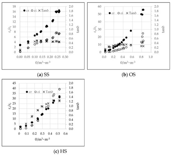
Figure 1.
Laboratory tested relative complex permittivity (εr, εi) and loss tangent (tanδ) under different soil water content conditions of three soils, (a) SS, (b) OS, (c) HS.
For sandy soil (SS) and organic soil (OS), was much smaller compared to , and the loss tangent () remained below 0.5 across the tested moisture range. This indicates that SS and OS can be classified as dielectric lossless soils, where energy dissipation due to dielectric losses is minimal. The low dielectric loss in these soils is primarily attributed to their low clay content, which limits the mobility of ions and the associated conduction losses. As water content increases, the polarization of free water molecules dominates the dielectric response, leading to a nonlinear increase in . However, the absence of significant conductive components (e.g., clay minerals or dissolved salts) results in negligible and low values [27].
In contrast, humus soil (HS) exhibited more complex dielectric behavior. For θ < 0.3 m3/m3, was smaller than , which was similar to SS and OS. However, when θ exceeded 0.3 m3/m3, surpassed , and reached a maximum value of approximately 1.26. The high dielectric loss in HS is primarily due to its elevated clay content, which introduces conductive pathways for ion mobility. As the soil water content increases, the presence of clay minerals facilitates the dissolution of ions and enhances electrical conductivity, leading to significant energy dissipation and higher values [8].
The nonlinear increase in and with θ can be explained by the interaction between soil water and the soil matrix. At low moisture levels, water molecules are tightly bound to soil particles, resulting in limited polarization and low permittivity. As θ increases, free water becomes more abundant, enhancing the soil’s ability to polarize and store electrical energy, which drives the rapid increase in . For , the nonlinearity is influenced by the soil’s conductive properties. In low-clay soils (e.g., SS and OS), remains low due to limited ion mobility. In contrast, high-clay soils (e.g., HS) exhibit a sharp increase in at higher θ values due to the activation of conductive pathways and the associated energy losses.
As established in Section 2.1, a linear relationship exists between soil water content () and the square root of relative permittivity () for any soil type. This relationship is expressed by the Soil Refractive Index (SRI) model as , where and are the slope and intercept parameters, respectively. Figure 2 illustrates the linear relationships between and for the three tested soils: sandy soil (SS), organic soil (OS), and humus soil (HS). The results demonstrate that θ increases linearly with for all three soils, with coefficients of determination (R²) close to 1, indicating an excellent fit. The root-mean-square errors (RMSE) for SS, OS, and HS were 0.008, 0.021, and 0.015, respectively, confirming the suitability of the SRI model for these soils, including the high dielectric loss soil (HS).
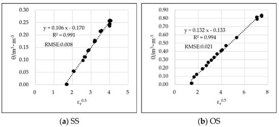
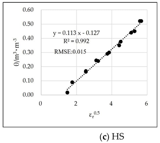
Figure 2.
The linear relationship fitting results between θ and for (a) SS, (b) OS, and (c) HS.
The slope values for SS, OS, and HS were 0.106, 0.132, and 0.113, respectively. These values are primarily controlled by the relative permittivity of soil water (), which is consistent across all soils. The slight variations in slope can be attributed to the random errors in data fitting.
The intercept values for SS, OS, and HS were −0.170, −0.133, and −0.127, respectively. These values are influenced by soil porosity () and the relative permittivity of the soil matrix (). SS, with the highest bulk density (1.523 g/cm3) and lowest porosity (0.430), exhibited the lowest intercept, reflecting its compact structure and limited pore space. In contrast, OS and HS, with higher porosities (0.870 and 0.720, respectively), had higher intercepts. However, the relationship between intercept and porosity for OS and HS appears counterintuitive, as OS, with the highest porosity (0.870), had a slightly lower intercept (−0.133) compared to HS (−0.127). This discrepancy may be attributed to random errors in the soil testing process or the influence of other factors, such as organic matter content and soil texture, which can affect the dielectric properties of the soil. Additionally, the linear fitting process optimizes the slope and intercept to minimize RMSE, which may result in slight deviations from the expected trend.
Assuming the tested soils are dielectric lossless, the slope parameter in the SRI model is primarily determined by the relative permittivity of soil water (), which is a function of temperature (T) and salinity (S). Based on the laboratory measurements by Lane and Saxton [30], the relationships are expressed as
For pure water, and . At room temperature (20 °C), the calculated = 79.8, resulting in for dielectric lossless soils. The SRI model for the tested soils can thus be theoretically determined as
The intercept parameter was calculated for each soil water level with averaged values of −0.229, −0.110, and −0.174 for SS, OS, and HS, respectively. The final SRI models for the three soils are
The soil water content calibration lines based on Equation (15) are compared with laboratory-measured results in Figure 3. The results show that can be accurately calculated using the theoretically determined for all three soils, including HS, which exhibits relatively high dielectric losses. The RMSE values for SS, OS, and HS are 0.018 m3/m3, 0.024 m3/m3, and 0.024 m3/m3, respectively. Although these RMSE values are slightly higher than those obtained from direct linear fitting (Figure 2), the differences are negligible (≤0.01 m3/m3), demonstrating the robustness of the SRI model.
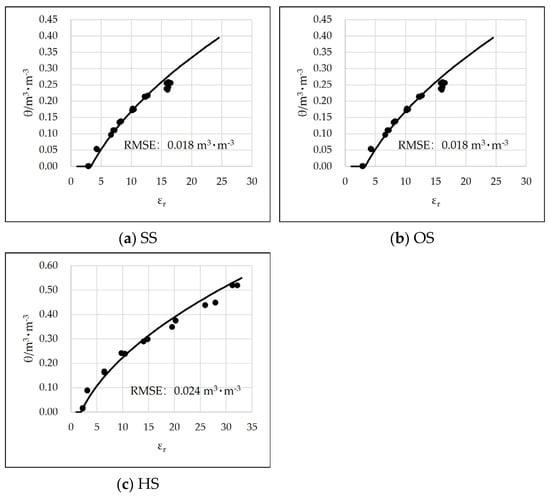
Figure 3.
Comparison between the measured and calculated results with SRI model for (a) SS, (b) OS, and (c) HS.
3.2. Verification with Existing Equations
To evaluate the applicability of the SRI model, comparisons were made with existing soil water content calculation equations for mineral and organic soils (Table 2).
For mineral soils, the equations provided by Topp et al. [11] and Malicki et al. [31] are similar to the SRI model with intercepts (B) and root-mean-square errors (RMSE) of −0.216 (0.019) and −0.194 (0.015), respectively. The absolute errors of the SRI model compared to the Topp equation ranged from −0.025 to 0.026, while those compared to the Malicki equation ranged from −0.024 to 0.027 (Figure 4a,b). In contrast, the Roth et al. [12] equation showed a larger deviation from the SRI model, with B = −0.206 and RMSE = 0.025, and absolute errors ranging from −0.031 to 0.037 (Figure 4c). These deviations likely stem from laboratory test errors and the influence of clay content. For instance, both the Topp and Roth equations are cubic empirical fitting formulas, which are strictly constrained by measured data and calibrated using soils with varying clay contents. Topp’s experiment included nine type soils with clay contents ranging from 9% to 66%, while Roth’s experiment also included nine type soils with clay contents ranging from 2% to 46%. Clay, a typical dielectric loss medium due to its high bound water content and electrical conductivity, significantly affects the dielectric properties of soils.
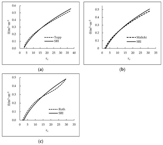
Figure 4.
Comparison between SRI model and equations published by (a)Topp, (b) Malicki and (c) Roth for mineral soils.
Bound water exhibits much lower dielectric permittivity compared to free water with its lower limit likely similar to that of ice (≈3.2) [32]. Dobson et al. found good agreement between theory and experiment for bound water dielectric permittivity in the range of 20 to 40 [20]. Due to the influence of bound water and the relatively high conductivity of clay, the loss tangent () cannot be neglected for clay-rich soils. Consequently, the slope parameter () in the SRI model deviates from the theoretically calculated value of 0.126 for such soils.
Table 2.
Comparison and validation with previously published equations.
Table 2.
Comparison and validation with previously published equations.
| Source | Original Equation Form | Soil Type | ρ/φ | SRI | RMSE |
|---|---|---|---|---|---|
| Topp et al [11] | Mineral soils | 1.25/ND | 0.019 | ||
| Roth et al. [12] | Mineral soils | 1.429/0.443 | 0.025 | ||
| Malicki et al. [31] | Mineral soils | 1.340/0.481 | 0.015 | ||
| Topp et al. [11] | Organic soils | 0.422/ND | 0.020 | ||
| Roth et al. [12] | Organic soils | 0.397/0.672 | 0.009 | ||
| Malicki et al. [31] | Organic soils | 0.240/0.824 | 0.008 | ||
| Schaap et al. [33] | Organic soils | 0.124/0.905 | 0.012 |
Figure 5a compares the SRI model (A = 0.126, B = −0.215) with the Topp equation for sandy loam, which can be considered a dielectric lossless soil. The SRI calibration line aligns well with the Topp equation with an RMSE of 0.010. In contrast, Figure 5b compares the SRI model (A = 0.126, B = −0.212) with the Topp equation for heavy clay soil (66% clay content), which exhibits high dielectric loss due to the electrical conductivity of moist clay. At low soil water content (θ < 0.2), the SRI model calculated lower water content than the Topp equation, while at high water content (θ > 0.4), the Topp equation yielded lower values than the SRI model. This discrepancy arises because the theoretical value of A = 0.126 is unsuitable for heavy clay soils.
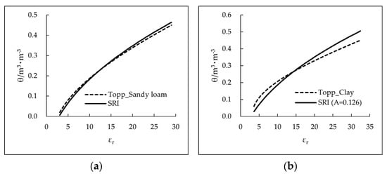
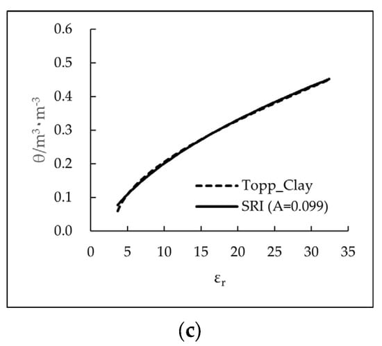
Figure 5.
Comparison between SRI model ( and Topp equation for (a) sandy loam, (b) clay, (c) SRI model () and Topp equation for clay.
For clayey soils, the actual value of A in the SRI model is challenging to determine theoretically due to the variation in with water content in dielectric loss soils. However, based on the general form of the SRI model (Equation (10)), the relationship between and remains linear: , where both A and B are unknown variables. By linear fitting, we obtained A = 0.099 and B = −0.112 for Topp’s heavy clay soil. Figure 5c shows that the SRI model with these modified parameters perfectly matches the Topp equation for heavy clay soil with an RMSE of 0.005.
For organic soils, the comparison between the Topp equation and the SRI model yielded results similar to those for mineral soils. Assuming , the calculated with an RMSE of 0.02. Analysis of the original data from Topp’s experiment revealed that errors primarily occurred at low soil water content levels (θ < 0.15) (Figure 6a). These errors are likely due to laboratory-tested heterogeneity at low water content levels. The Roth equation for organic soil can be equivalently expressed as the SRI model with and , yielding an RMSE of 0.009 (Figure 6b). Similarly, Malicki’s equation for organic soil, a linear fit between and at bulk densities of 0.2–0.3 g/cm3, can be converted into the SRI model with , , and RMSE = 0.008 (Figure 6c). Schaap et al. [33] proposed that the square root of soil relative permittivity is a volumetrically weighted average of different soil components and used this assumption to calibrate forest floor soils. Their linear fitting yielded values ranging from 0.123 to 0.228 for different forest organic soil samples, attributing deviations from the theoretical value of to the influence of bound water, which has lower permittivity. To address deviations at very low permittivity levels ( < 2), Schaap’s equation incorporated an empirical adjustment factor. Even when is set to the theoretical value for free water, Schaap’s equation for forest floor organic soils can still be represented by the SRI model with and RMSE = 0.012 (Figure 6d). The relatively large deviation at very low water content levels is likely due to soil sample shrinkage, as described by the authors.
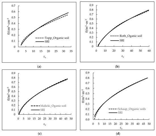
Figure 6.
Comparison between SRI model and (a) Topp equation, (b) Roth equation, (c) Malicki equation and (d) Schaap equation for organic soil.
Through comparisons with previously published results, we conclude that the SRI model, derived from electromagnetic wave propagation, is applicable to both mineral and organic soils. The model requires the determination of two parameters: the slope () and intercept (). For most soils, can be theoretically determined based on the relative permittivity of soil water, yielding a value of 0.126 at room temperature. However, for heavy clay soils, is smaller than 0.126 due to the influence of dielectric loss caused by clay.
3.3. Influence of Soil Porosity
For dielectric lossless soils, the intercept parameter in SRI model can be expressed as
We can find that is determined by three key factors: the slope parameter , the relative permittivity of the soil matrix , and the soil porosity . Since typically ranges between 3 and 10, with most published data clustering around 5 [1,34], and is constant (), the primary influence on comes from soil porosity . Specifically, for dielectric lossless soils, exhibits a linear increase with increasing . This relationship highlights the critical role of soil porosity in determining the intercept parameter , making it a key variable for accurate soil water content estimation.
Figure 7 presents the statistical relationship between soil porosity and the corresponding values of . The dataset includes three soil types (SS, OS, HS) tested in this study as well as mineral and organic soils analyzed by Roth et al. [12], Malicki et al. [31], and Schaap et al. [33]. The results demonstrate a clear linear trend with increasing as soil porosity rises. For example, the sandy soil tested in our study, with a porosity of 0.430, yielded the lowest intercept value of . In contrast, the forest floor organic soils examined by Schaap et al. exhibited the highest intercept value of . These findings underscore the variability of across different soil types and its strong dependence on soil porosity.
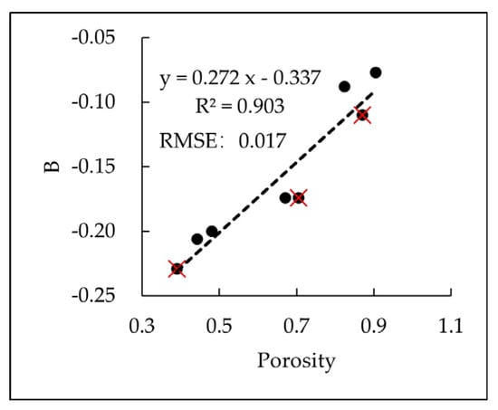
Figure 7.
Statistical relationship between soil porosity and parameter B in SRI model for different soil (red cross marks represents our tested three soils, SS, OS and HS).
Based on the compiled data, the linear fitting function for the intercept parameter can be expressed as
The root mean square error (RMSE) and mean absolute error (MAE) for this fitting are 0.017 and 0.014, respectively. This indicates that if soil porosity is used to estimate , the average error in soil water content calculations using the SRI model is within 0.02. Such a low error margin highlights the robustness and reliability of the SRI model for diverse soil types. This enhances the applicability of the SRI model in real-world scenarios, where soil properties can vary significantly.
4. Discussion
The SRI model provides a robust framework for estimating soil water content () based on relative permittivity (). The slope parameter and intercept parameter are critical to the model’s accuracy and applicability. Below, we provide a detailed analysis of how these parameters vary under different soil conditions and their implications for soil water content estimation.
The slope parameter is primarily determined by the relative permittivity of soil water (), which is a function of temperature and salinity. Variations in soil composition (e.g., clay content, salt) can introduce minor deviations. For example, in soils with high clay content, the presence of bound water and ionic conductivity may slightly alter the effective permittivity, leading to small changes in . However, our experimental results for sandy soil (SS), organic soil (OS), and humus soil (HS) showed that remained relatively stable (0.106–0.132), confirming its robustness across diverse soil types.
The intercept parameter is influenced by soil porosity () and the relative permittivity of the soil matrix (). Soil porosity is the primary factor affecting . In our experiments, increased linearly with φ, as demonstrated by the values for SS (, ), HS (,), and OS (, ). This trend aligns with the theoretical expectation that higher porosity enhances the soil’s ability to store water, leading to a less negative intercept. Although varies little across different soil types, minor differences can still influence . For instance, soils with higher organic matter content (e.g., OS) may exhibit slightly lower due to the lower permittivity of organic materials compared to mineral components.
For dielectric lossless soils, the SRI model simplifies to , where can be estimated using soil porosity or dry soil permittivity. This simplification makes the model highly practical for field applications particularly in soils with low clay content and minimal dielectric losses.
While the SRI model performs well for high dielectric loss soils like HS, further research is needed to refine the estimation of and under such conditions. Potential approaches include incorporating corrections for ionic conductivity and bound water effects.
5. Conclusions
The relationship between soil water content () and relative permittivity () is fundamental to the accurate determination of soil moisture using electromagnetic wave-based techniques. This study proposed the SRI model, which theoretically expresses the - relationship as for any soil type. The SRI model was validated through laboratory experiments on three distinct soils—sandy soil (SS) as a representative mineral soil, and two organic soils (OS and HS)—as well as through comparisons with previously published calibration equations. The results demonstrated that the SRI model accurately describes the - relationship for both mineral and organic soils, highlighting its broad applicability.
In the SRI model, two parameters—slope () and intercept ()—are critical for soil water content calculation. For dielectric lossless soils, the slope parameter is determined by the relative permittivity of soil water (). At room temperature (20 °C), where , the theoretical value of is 0.126. For dielectric loss soils, decreases due to the influence of the loss tangent on electromagnetic wave propagation speed. Interestingly, our experimental results revealed that soils with a loss tangent as high as 1.26 can still be treated as dielectric lossless for soil water content calculations, expanding the practical applicability of the SRI model.
The intercept parameter is influenced by soil porosity () and soil matrix relative permittivity (). Since varies little across different soil types, is primarily determined by and increases linearly with porosity. In practice, can be calculated using dry soil relative permittivity, estimated from measured - data, or derived from soil porosity. This flexibility enhances the utility of the SRI model in diverse field conditions.
While this study provides a robust framework for soil water content estimation using the SRI model, the following limitations and future research directions are worth noting. Our experiments indicated that soils with a loss tangent up to 1.26 can be treated as dielectric lossless. However, due to the limited number of soil samples tested, a definitive threshold for the maximum loss tangent value that qualifies a soil as dielectric lossless remains unclear. Future studies should investigate a wider range of soil types to establish a more precise threshold. Although the SRI model is applicable to dielectric loss soils, this study did not establish a precise method for calculating or estimating the model parameters (e.g., and ) for such soils. Future research should focus on developing accurate parameter estimation techniques for dielectric loss soils to further extend the model’s applicability.
In conclusion, the SRI model offers a universal and theoretically grounded approach for estimating soil water content based on relative permittivity. Its applicability to both mineral and organic soils, combined with its simplicity and flexibility, makes it a valuable tool for soil moisture monitoring in agriculture, hydrology, and environmental science. Addressing the limitations outlined above will further enhance the model’s utility and pave the way for innovative applications in soil science and related fields.
Author Contributions
The contribution of each author is listed as below. Conceptualization, E.D. and L.Z.; methodology, E.D.; validation, E.D.; formal analysis, E.D., R.L. and Y.X.; investigation, D.Z., Z.L., Y.Z. (Yuxin Zhang), Z.X., Y.X., G.L. and Y.Z. (Yonghua Zhao); resources, T.W., X.W. and G.H.; data curation, T.W. and X.W.; writing—original draft preparation, E.D.; writing—review and editing, G.H., L.Z., D.Z., Z.X., L.W., T.W. and X.W.; supervision, T.W. and X.W.; project administration, L.Z. and G.H.; funding acquisition, L.Z. and G.H. All authors have read and agreed to the published version of the manuscript.
Funding
This research was supported by the National Natural Science Foundation of China (grant no. 41931180), the Second Tibet Plateau Scientific Expedition and Research (STEP) program (grant no. 2019QZKK0201), part of this work was also supported by the National Natural Science Foundation of China (grant no. 42322608, 42071093).
Data Availability Statement
All data used in this manuscript were presented in the context, figures and tables.
Conflicts of Interest
The authors declare no conflicts of interest.
References
- Huisman, J.A.; Hubbard, S.S.; Redman, J.D.; Annan, A.P. Measuring Soil Water Content with Ground Penetrating Radar: A Review. Vadose Zone J. 2003, 2, 476–491. [Google Scholar] [CrossRef]
- Du, E.; Zhao, L.; Zou, D.; Li, R.; Wang, Z.; Wu, X.; Hu, G.; Zhao, Y.; Liu, G.; Sun, Z. Soil Moisture Calibration Equations for Active Layer GPR Detection—A Case Study Specially for the Qinghai–Tibet Plateau Permafrost Regions. Remote Sens. 2020, 12, 605. [Google Scholar] [CrossRef]
- Ardekani, M.R.M. Off- and on-Ground GPR Techniques for Field-Scale Soil Moisture Mapping. Geoderma 2013, 200–201, 55–66. [Google Scholar] [CrossRef]
- Shamir, O.; Goldshleger, N.; Basson, U.; Reshef, M. Laboratory Measurements of Subsurface Spatial Moisture Content by Ground-Penetrating Radar (GPR) Diffraction and Reflection Imaging of Agricultural Soils. Remote Sens. 2018, 10, 1667. [Google Scholar] [CrossRef]
- Dalton, F.N. Development of Time-Domain Reflectometry for Measuring Soil Water Content and Bulk Soil Electrical Conductivity. In SSSA Special Publications; Clarke Topp, G., Daniel Reynolds, W., Green, R.E., Eds.; Soil Science Society of America: Madison, WI, USA, 2012; pp. 143–167. ISBN 978-0-89118-925-1. [Google Scholar]
- Noborio, K. Measurement of Soil Water Content and Electrical Conductivity by Time Domain Reflectometry: A Review. Comput. Electron. Agric. 2001, 31, 213–237. [Google Scholar] [CrossRef]
- Qin, A.; Ning, D.; Liu, Z.; Duan, A. Analysis of the Accuracy of an FDR Sensor in Soil Moisture Measurement under Laboratory and Field Conditions. J. Sens. 2021, 2021, 6665829. [Google Scholar] [CrossRef]
- Kelleners, T.J.; Soppe, R.W.O.; Robinson, D.A.; Schaap, M.G.; Ayars, J.E.; Skaggs, T.H. Calibration of Capacitance Probe Sensors Using Electric Circuit Theory. Soil. Sci. Soc. Amer J. 2004, 68, 430–439. [Google Scholar] [CrossRef]
- Robinson, D.A.; Gardner, C.M.K.; Evans, J.; Cooper, J.D.; Hodnett, M.G.; Bell, J.P. The Dielectric Calibration of Capacitance Probes for Soil Hydrology Using an Oscillation Frequency Response Model. Hydrol. Earth Syst. Sci. 1998, 2, 111–120. [Google Scholar] [CrossRef]
- Li, Z.-L.; Leng, P.; Zhou, C.; Chen, K.-S.; Zhou, F.-C.; Shang, G.-F. Soil Moisture Retrieval from Remote Sensing Measurements: Current Knowledge and Directions for the Future. Earth-Sci. Rev. 2021, 218, 103673. [Google Scholar] [CrossRef]
- Topp, G.C.; Davis, J.L.; Annan, A.P. Electromagnetic Determination of Soil Water Content: Measurements in Coaxial Transmission Lines. Water Resour. Res. 1980, 16, 574–582. [Google Scholar] [CrossRef]
- Roth, C.H.; Malicki, M.A.; Plagge, R. Empirical Evaluation of the Relationship between Soil Dielectric Constant and Volumetric Water Content as the Basis for Calibrating Soil Moisture Measurements by TDR. J. Soil Sci. 1992, 43, 1–13. [Google Scholar] [CrossRef]
- Almeida, K.S.S.A.D.; Souza, L.D.S.; Paz, V.P.D.S.; Coelho Filho, M.A.; Hoces, E.H. Models for Moisture Estimation in Different Horizons of Yellow Argisol Using TDR. Semina Ciênc. Agrár. 2017, 38, 1727–1736. [Google Scholar] [CrossRef][Green Version]
- Guo, Y.; Xu, S.; Shan, W. Development of a Frozen Soil Dielectric Constant Model and Determination of Dielectric Constant Variation during the Soil Freezing Process. Cold Reg. Sci. Technol. 2018, 151, 28–33. [Google Scholar] [CrossRef]
- He, H.; Zou, W.; Jones, S.B.; Robinson, D.A.; Horton, R.; Dyck, M.; Filipović, V.; Noborio, K.; Bristow, K.; Gong, Y.; et al. Critical Review of the Models Used to Determine Soil Water Content Using TDR-Measured Apparent Permittivity. In Advances in Agronomy; Elsevier: Amsterdam, The Netherlands, 2023; Volume 182, pp. 169–219. ISBN 978-0-443-19268-5. [Google Scholar]
- Loor, G.P.D. Dielectric Properties of Heterogeneous Mixtures Containing Water. J. Microw. Power 1968, 3, 67–73. [Google Scholar] [CrossRef]
- Loor, G.P.D. Dielectric Properties of Heterogeneous Mixtures with a Polar Constituent. Appl. Sci. Res. Sect. B 1964, 11, 310–320. [Google Scholar] [CrossRef]
- Friedman, S.P. A Saturation Degree-dependent Composite Spheres Model for Describing the Effective Dielectric Constant of Unsaturated Porous Media. Water Resour. Res. 1998, 34, 2949–2961. [Google Scholar] [CrossRef]
- Jones, S.B.; Friedman, S.P. Particle Shape Effects on the Effective Permittivity of Anisotropic or Isotropic Media Consisting of Aligned or Randomly Oriented Ellipsoidal Particles. Water Resour. Res. 2000, 36, 2821–2833. [Google Scholar] [CrossRef]
- Dobson, M.; Ulaby, F.; Hallikainen, M.; El-rayes, M. Microwave Dielectric Behavior of Wet Soil-Part II: Dielectric Mixing Models. IEEE Trans. Geosci. Remote Sens. 1985, GE-23, 35–46. [Google Scholar] [CrossRef]
- He, H.; Dyck, M.; Zhao, Y.; Si, B.; Jin, H.; Zhang, T.; Lv, J.; Wang, J. Evaluation of Five Composite Dielectric Mixing Models for Understanding Relationships between Effective Permittivity and Unfrozen Water Content. Cold Reg. Sci. Technol. 2016, 130, 33–42. [Google Scholar] [CrossRef]
- Comas, X.; Slater, L.; Reeve, A. Spatial Variability in Biogenic Gas Accumulations in Peat Soils Is Revealed by Ground Penetrating Radar (GPR). Geophys. Res. Lett. 2005, 32, 2004GL022297. [Google Scholar] [CrossRef]
- Parsekian, A.D.; Slater, L.; Giménez, D. Application of Ground-penetrating Radar to Measure Near-saturation Soil Water Content in Peat Soils. Water Resour. Res. 2012, 48, 2011WR011303. [Google Scholar] [CrossRef]
- Birchak, J.R.; Gardner, C.G.; Hipp, J.E.; Victor, J.M. High Dielectric Constant Microwave Probes for Sensing Soil Moisture. Proc. IEEE 1974, 62, 93–98. [Google Scholar] [CrossRef]
- Whalley, W.R. Considerations on the Use of Time-domain Reflectometry (TDR) for Measuring Soil Water Content. J. Soil Sci. 1993, 44, 1–9. [Google Scholar] [CrossRef]
- Brovelli, A.; Cassiani, G. Effective Permittivity of Porous Media: A Critical Analysis of the Complex Refractive Index Model. Geophys. Prospect. 2008, 56, 715–727. [Google Scholar] [CrossRef]
- Pérez, M.; Mendez, D.; Avellaneda, D.; Fajardo, A.; Páez-Rueda, C.I. Time-Domain Transmission Sensor System for on-Site Dielectric Permittivity Measurements in Soil: A Compact, Low-Cost and Stand-Alone Solution. HardwareX 2023, 13, e00398. [Google Scholar] [CrossRef]
- Blonquist, J.M.; Jones, S.B.; Robinson, D.A. Standardizing Characterization of Electromagnetic Water Content Sensors: Part 2. Evaluation of Seven Sensing Systems. Vadose Zone J. 2005, 4, 1059–1069. [Google Scholar] [CrossRef]
- Campbell, J.E. Dielectric Properties and Influence of Conductivity in Soils at One to Fifty Megahertz. Soil Sci. Soc. Am. J. 1990, 54, 332–341. [Google Scholar] [CrossRef]
- Lane, J.A.; Saxton, J.A. Dielectric Dispersion in Pure Polar Liquids at Very High Radio Frequencies—III. The Effect of Electrolytes in Solution. Proc. R. Soc. Lond. A 1952, 214, 531–545. [Google Scholar] [CrossRef]
- Malicki, M.A.; Plagge, R.; Roth, C.H. Improving the Calibration of Dielectric TDR Soil Moisture Determination Taking into Account the Solid Soil. Eur. J Soil Sci. 1996, 47, 357–366. [Google Scholar] [CrossRef]
- Dirksen, C.; Dasberg, S. Improved Calibration of Time Domain Reflectometry Soil Water Content Measurements. Soil Sci. Soc. Am. J. 1993, 57, 660–667. [Google Scholar] [CrossRef]
- Schaap, M.G.; De Lange, L.; Heimovaara, T.J. TDR Calibration of Organic Forest Floor Media. Soil Technol. 1997, 11, 205–217. [Google Scholar] [CrossRef]
- Heimovaara, T.J. Frequency Domain Analysis of Time Domain Reflectometry Waveforms: 1. Measurement of the Complex Dielectric Permittivity of Soils. Water Resour. Res. 1994, 30, 189–199. [Google Scholar] [CrossRef]


Disclaimer/Publisher’s Note: The statements, opinions and data contained in all publications are solely those of the individual author(s) and contributor(s) and not of MDPI and/or the editor(s). MDPI and/or the editor(s) disclaim responsibility for any injury to people or property resulting from any ideas, methods, instructions or products referred to in the content. |
© 2025 by the authors. Licensee MDPI, Basel, Switzerland. This article is an open access article distributed under the terms and conditions of the Creative Commons Attribution (CC BY) license (https://creativecommons.org/licenses/by/4.0/).