Forecasting the River Ice Break-Up Date in the Upper Reaches of the Heilongjiang River Based on Machine Learning

Abstract

Ice-jam floods (IJFs) are a significant hydrological phenomenon in the upper reaches of the Heilongjiang River, posing substantial threats to public safety and property. This study employed various feature selection techniques, including the Pearson correlation coefficient (PCC), Grey Relational Analysis (GRA), mutual information (MI), and stepwise regression (SR), to identify key predictors of river ice break-up dates. Based on this, we constructed various machine learning models, including Extreme Gradient Boosting (XGBoost), Backpropagation Neural Network (BPNN), Random Forest (RF), and Support Vector Regression (SVR). The results indicate that the ice reserves in the Oupu to Heihe section have the most significant impact on the ice break-up date in the Heihe section. Additionally, the accumulated temperature during the break-up period and average temperature before river ice break-up are identified as features closely related to the river’s opening in all four feature selection methods. The choice of feature selection method notably impacts the performance of the machine learning models in predicting the river ice break-up dates. Among the models tested, XGBoost with PCC-based feature selection achieved the highest accuracy (RMSE = 2.074, MAE = 1.571, R² = 0.784, NSE = 0.756, TSS = 0.950). This study provides a more accurate and effective method for predicting river ice break-up dates, offering a scientific basis for preventing and managing IJF disasters.

1. Introduction

Ice-jam floods (IJFs) are a hydrological phenomenon caused by the obstruction of water flow due to the accumulation and blockage of ice, which is mainly manifested through the rupture, movement, and evolution of river ice due to sudden changes in temperature and other environmental factors [1,2,3]. In recent years, IJFs have become increasingly frequent in many high-latitude and high-altitude regions due to global warming [4,5]. At the same time, owing to rapid population growth and accelerated socio-economic development, higher requirements have been placed on the prevention of IJF risks [6,7,8]. Accurately predicting river ice break-up dates can aid in identifying and assessing potential IJF disasters in advance, optimizing water resource management, and assisting ecological protection departments in implementing appropriate measures to safeguard aquatic habitats and maintain ecological balance. Consequently, developing precise tools to predict river ice break-up dates and evaluate the impact of various factors on their variability has become a complex and critical focus of IJF research.

At present, two primary types of models are utilized to predict river ice break-up dates: numerical simulation methods and statistical methods [9]. Numerical simulation methods employ physical models that account for the mechanics and thermodynamics of ice layers, predicting ice break-up by simulating the rupture process. Common numerical simulation models, such as RIVICE, DYNARICE, ICEJAM, and RIVJAM [10,11,12,13], offer detailed dynamic predictions. However, in practice, acquiring real-time and accurate data from field observations is frequently challenging due to adverse environmental conditions and the complexity of ice-flooding regions [14,15]. This scarcity of data constrains the accuracy and reliability of the models, diminishing their effectiveness. Furthermore, a significant limitation of these traditional hydrological models is the complexity associated with parameter calibration. Accurate parameter calibration is crucial for reliable predictions; however, this process often requires substantial time and expertise. Statistical methodology refers to methods for collecting, collating, analyzing, and interpreting statistical data and for drawing certain conclusions about the issues they reflect. Statistical methods do not require a large number of boundary initial conditions or a variety of complex technical parameters and can, therefore, be adapted to many ambiguous background problems. Lei et al. [16] correlated historical hydrometeorological data with the river ice break-up dates and established empirical correlation diagrams between the factors with higher coefficients and the date of river opening for forecasting. The accuracy rate of their forecasting was 72%, demonstrating the effectiveness of statistical methods in addressing complex environmental problems with limited data and uncertainties. However, statistical methods have their own limitations. They often rely on assumptions about data distribution, such as normality or independence, which may not always hold true for real-world data. Furthermore, the accuracy of statistical conclusions is contingent on data quality, and issues such as measurement errors, missing values, or noise can undermine the validity of results. In addition, statistical methods typically focus on correlation rather than causation, and without careful experimental design or control for confounding variables, they may lead to misleading conclusions.

In recent years, the development of Artificial Intelligence (AI) has opened new paths and demonstrated great potential for ice forecasting [17]. By leveraging its ability to process large datasets and analyze complex systems, AI is expected to improve the accuracy of river ice break-up forecasting and enhance model interpretability. Smith et al. [18] used Bayesian logistic regression to estimate the frequency of IJFs while considering uncertainty in the historical record, thereby making the flood frequency analysis more accurate. Liu et al. [19] combined a Long Short-Term Memory (LSTM) network with a CEEMDAN-decomposed time series to predict river ice break-up. Shevnina and Solov’eva [20] investigated the correlation between the autumn accumulation temperature and ice break-up dates, achieving a probability of correct prediction between 67% and 86%. The variability of time-series data has increased due to more unpredictable weather patterns and a higher frequency of extreme events caused by global warming. However, multi-feature forecasting can provide more accurate results by combining and analyzing multiple features and adapting to changes in different data sources and forecasting needs [21,22,23,24]. As a data-driven approach, choosing appropriate predictors is the key to successful prediction [25,26]. However, the mechanism of IJFs is complex and influenced by multiple factors, with intricate nonlinear relationships among them, making feature engineering particularly important [27]. Effective feature engineering enables machine learning (ML) models to better capture nonlinear relationships, eliminate redundant features, and minimize the impact of irrelevant inputs on performance [28,29,30]. Ji et al. [31] utilized the correlation coefficient method for feature selection and applied a fuzzy optimization neural network to predict the river closure at the estuary of the Three Lakes section of the Yellow River, achieving a prediction accuracy of 80%. Li et al. [32] studied the method of determining the forecasting factors in the process of ice forecasting by using AI technology and used Back Propagation Neural Network (BPNN) to forecast river ice break-up in the Mohe section of the Heilongjiang River with a prediction accuracy rate of between 50% and 75%.

Although IJFs have been extensively studied by many scholars [33,34,35], their suddenness, wide impact and erratic characteristics still limit the accuracy of existing forecasting models [36,37,38]. Most studies have employed a single feature selection method or a single model for forecasting, with limited consideration of integrating multiple feature selection methods and ML models. In ice forecasting, complex and nonlinear relationships often exist between the forecast target and influencing factors, and a single method may fail to capture all features contributing to the model. Furthermore, different ML models with different assumptions, ways of handling data, and varying adaptability to specific problems may also affect the final prediction. Therefore, in this study, multiple feature selection techniques (PCC, GRA, MI, and SR) were used to screen the contributing factors to reduce the bias caused by a single method, and multiple ML models (XGBoost, BPNN, RF, and SVR) were constructed on this basis. The aim was to elucidate the changing characteristics of river ice break-up dates in the upper Heilongjiang River, along with their influencing factors, and to maximize prediction accuracy. Enhancing disaster prevention capabilities and exploring the complementary advantages of diverse methods can offer valuable insights for improving ML models.

2. Material and Methods

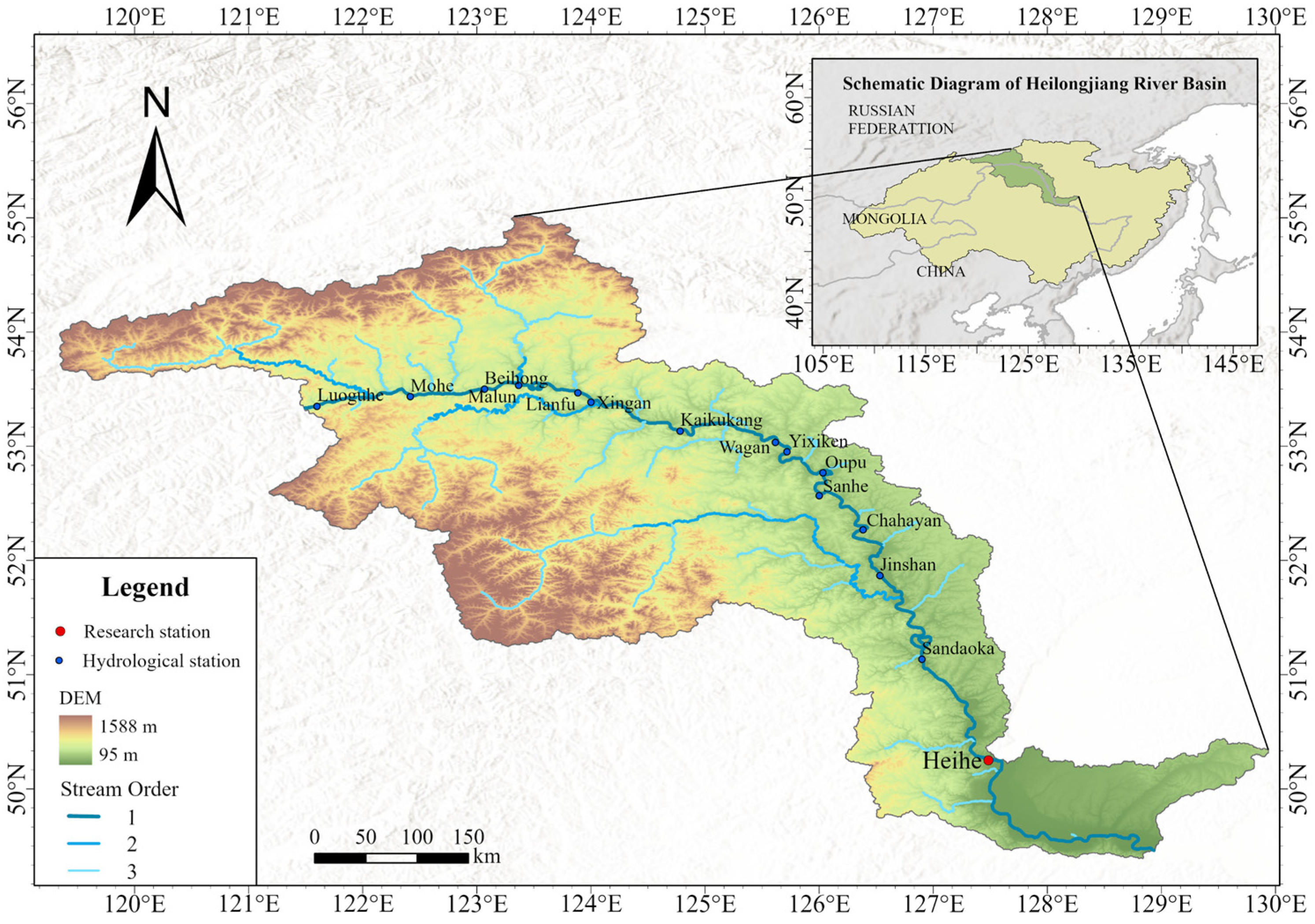
2.1. Overview of the Study Area

The main course of the Heilongjiang River starts at the confluence of the Shilka and Argun Rivers and extends to Khabarovsk, Russia, with a total length of 2821 km. Winter lasts for about 8 months, with an ice-covered period averaging over 150 days. Due to its unique river channel shape, flow rate, and hydrometeorological conditions, IJFs occur frequently. From 1940 to 2023, there were 34 years of severe IJF disasters, which greatly impacted the production and lives of the local people [39,40].

Heihe is located in the mid-temperate zone (Figure 1) [41], where the river typically freezes in November and begins thawing in late April or early May. The annual average temperature ranges from −1.3 °C to 0.4 °C, with extreme minimum temperatures dropping as low as −45 °C. The annual precipitation averages around 500 mm, mostly concentrated during the summer months. Heihe is located directly across from Russia’s Amur Region. It plays a “leading” role in early warning and forecasting for flood control, flood prevention, and ice jam disaster mitigation in the Heilongjiang River. Historically, IJFs in the Heilongjiang River have caused significant harm to the people along its banks, and the Heihe section alone has experienced ice dams five times, resulting in severe damage.

2.2. Data Acquisition and Processing

River ice break-up dates, water levels, and ice thicknesses for the Heihe section were obtained from the Heilongjiang Hydrology and Water Resources Center. Daily atmospheric reanalysis data, including temperature, wind speed, snow depth, cloudiness, and precipitation, were sourced from the ERA5-Land dataset provided by the European Centre for Medium-Range Weather Forecasts (ECMWF), with a horizontal resolution of 0.1° × 0.1°. This dataset is available at https://cds.climate.copernicus.eu, accessed on 1 June 2023. River channel data were acquired from the Global River Widths from Landsat Database, which can be accessed on Zenodo (https://doi.org/10.1126/science.aat0636). Data analysis and processing were carried out using Python 3.8, Origin 2022, and Excel 2021.

2.3. Calculation of Ice Reserves

During winter, as the temperature drops, a significant amount of water is stored in rivers as solid ice, referred to as ice reserves. Ice reserves serve as an indicator of the amount of ice accumulated in rivers during the winter. In order to obtain an accurate picture of the changes in ice reserves and their impact on the river ice break-up, first, two-dimensional calculations were performed using DEM data with 12.5 m resolution. The area of the river that was frozen was determined based on the frozen water level recorded at each hydrological station during the previous year. Second, the measured maximum ice thickness at the hydrological stations was used to calibrate the ice thickness growth coefficient of the freezing degree day method in order to deduce the river ice thickness and ice reserves during the open river period. The formulas used to calculate ice reserves and ice thickness are provided below [42]:

$$h_m=\alpha \sqrt{FDD},$$

(1)

$$\Delta W_{ice}={\displaystyle {\int }_0^L{h}_{m}dA},$$

(2)

where h_m is the maximum ice thickness, m; α is the ice thickness growth factor, cm/(°C·d)^−0.5; FDD is the freezing degree days, °C·d; and A is the frozen area, m². Equation (2) can be expressed as follows:

$$W_{ice}={\displaystyle \sum _{i=1}^n\Delta W_{ice}}$$

(3)

2.4. Mann-Kendall Test

The Mann–Kendall test is a non-parametric method used to analyze trend characteristics and change points in data series. When using the Mann–Kendall algorithm to test broad trends in time series data, the trends are categorized as no apparent trend, increasing trend, or decreasing trend. The test compares the relative magnitude of the sample data rather than the data values themselves, so the underlying data does not need to follow a particular distribution or require the trend of change to be linear. The overall statistic S is calculated by comparing each pair of data points and is then normalized to a Z-value to assess whether a significant trend exists in the time-series data. This method is widely used in the analysis of hydrological and meteorological datasets [43].

2.5. Feature Selection Methods

Feature selection is a key step in improving the predictive power of a model and avoiding overfitting. The purpose of feature selection is to select the most representative and informative subset from a large number of features and remove redundant or irrelevant features. The evolution of ice conditions is affected by a variety of factors, and there is often a complex nonlinear relationship between forecast objects and disaster-causing factors. Twelve candidate factors were identified through a comprehensive analysis of the geographic location and ice condition characteristics of the Heilongjiang Heihe section (see

Table 1. Candidate factors for predicting the river ice break-up date.

Candidate Factors	Code
Accumulated temperature during the break-up period (°C)	X1
Date of positive temperature stabilization (d)	X2
Average temperature before river ice break-up (°C)	X3
Ice reserves (m3)	X4
Average wind speed during the break-up period (m/s)	X5
Average snow depth during the break-up period (mm)	X6
Precipitation prior to river freeze-up (mm)	X7
Precipitation during the river freeze-up period (mm)	X8
Precipitation before river ice break-up (mm)	X9
Precipitation during the break-up period (mm)	X10
Average cloud cover during the break-up period (0–1)	X11
Maximum ice thickness (cm)	X12

Note: ‘Prior to river freeze-up’ refers to October; ‘during the river freeze-up period’ refers to November through March of the following year; ‘before river ice break-up’ refers to March of the following year, and the ‘break-up period’ refers to April 1–20 of the following year.

). Next, Min-Max normalization [44] was applied to eliminate the dimensional differences between different features. Four feature selection methods were used to identify the features that significantly impact the ice break-up date in the Heihe section.

2.5.1. Pearson Correlation Coefficient

The Pearson correlation coefficient (PCC) is used to measure the linear correlation between two sets of data. It is calculated as the covariance between the two variables, divided by the product of their standard deviations. Its value ranges from −1 to 1.

After calculating the Pearson correlation coefficient, a significance test can also be conducted to assess the statistical significance of the correlation coefficient. These significance tests are designed to evaluate whether the observed correlation coefficient is sufficiently large to reject the presence of correlation due to random sampling errors [45]. If the correlation is not significant, a high coefficient may be meaningless and due to chance. Generally, a p-value of less than 0.05 is required to conclude that a significant relationship exists between the two datasets.

2.5.2. Grey Relational Analysis

Grey Relational Analysis (GRA) is a multi-factor statistical method used to measure the degree of association between factors of two systems as they change over time or across different objects. This association, known as the Grey Relational Grade (GRG), is higher when the trends of the two factors are consistent, indicating synchronous changes. Conversely, if the trends are dissimilar, the GRG is lower. The threshold is set to 0.3. This threshold is based on related studies [32,39], which suggest that a GRG value of 0.3 effectively excludes features with a low association with the river ice break-up date, thereby improving model accuracy, reducing computational complexity, and minimizing the risk of overfitting.

2.5.3. Mutual Information

Mutual Information (MI) is a concept in probability and information theory that is used to assess the degree of interdependence between two variables. Mutual information is calculated for each feature and the target variable, and the features are ranked according to the value of mutual information. A higher value of MI indicates a stronger dependency between the feature and the target variable.

For features with high MI values, permutation tests can be used to assess the statistical significance of the relationship. A small p-value (typically <0.05) indicates that the MI of the feature is significantly higher than expected under random conditions, confirming a strong relationship between the feature and the target variable.

2.5.4. Stepwise Regression

Stepwise Regression (SR) is a method for automatically screening variables that significantly affect the regression equation from a large set of available variables. SR begins with one independent variable and adds variables to the regression equation one by one, based on the significance of their effect on the dependent variable, y. After introducing a new variable, if any of the previously included variables are no longer significant, they will be removed. When previously introduced variables become insignificant due to the inclusion of subsequent variables, those variables are removed to ensure that the regression equation contains only significant variables before introducing new ones, ultimately leading to an optimal combination of variables.

In SR, the significance levels for adding (α) and removing (β) variables are typically set at 0.4. This threshold is based on related studies [32]. Studies indicate that the threshold of 0.4 can reflect the many-to-one relationships between various influencing factors and the river ice break-up dates.

2.6. Machine Learning Algorithms

ML refers to algorithms that automatically learn from data to make predictions or decisions. Datasets are typically divided into a training set and a test set. The training set is a dataset used to train an ML model so that it can learn the relationship between input features and target variables. The training process usually involves tuning the parameters of the model to minimize the model’s prediction error on the training set. The test set, on the other hand, is the dataset used to evaluate the performance of the ML model. The test set verifies the model’s ability to generalize to unseen data, i.e., its capacity to predict new, unknown data.

In our study, we utilized the ’random_state’ parameter to randomly partition the dataset into a training set (80%) and a test set (20%). Models were then constructed using XGBoost, BPNN, RF, and SVR. The details of the training and test datasets are provided in

Table 2. Dataset segmentation.

Dataset	Variable	Minimum	Maximum	Mean
Training Set	X1 (°C)	−65.51	115.18	20.06
	X2 (d)	−19	17	2
	X3 (°C)	−14.51	−1.68	−8.69
	X4 (m3)	2.55 × 108	3.21 × 108	2.88 × 108
	X5 (m/s)	2.13	3.71	2.87
	X6 (mm)	0	88.67	6.90
	X7 (mm)	7.13	102.27	35.71
	X8 (mm)	47.50	197.50	91.80
	X9 (mm)	1.40	38.00	13.67
	X10 (mm)	1.5	151.30	34.53
	X11 (0–1)	30.54	76.11	57.87
	X12 (cm)	85	1.75	120
Test Set	X1 (°C)	−38.64	84.12	29.39
	X2 (d)	−11	18	3
	X3 (°C)	−14.52	−3.84	−10.15
	X4 (m3)	2.79 × 108	3.18 × 108	2.98 × 108
	X5 (m/s)	2.39	3.37	2.83
	X6 (mm)	0	31.32	6.47
	X7 (mm)	8.95	86.47	38.57
	X8 (mm)	44.90	137	84.88
	X9 (mm)	2.40	26.90	14.15
	X10 (mm)	4.10	72.6	33.24
	X11 (0–1)	42.43	65.54	54.83
	X12 (cm)	78	173	119

Note: The river ice break-up date was converted to a numeric value, which is shown as the number of days to 1 April.

.

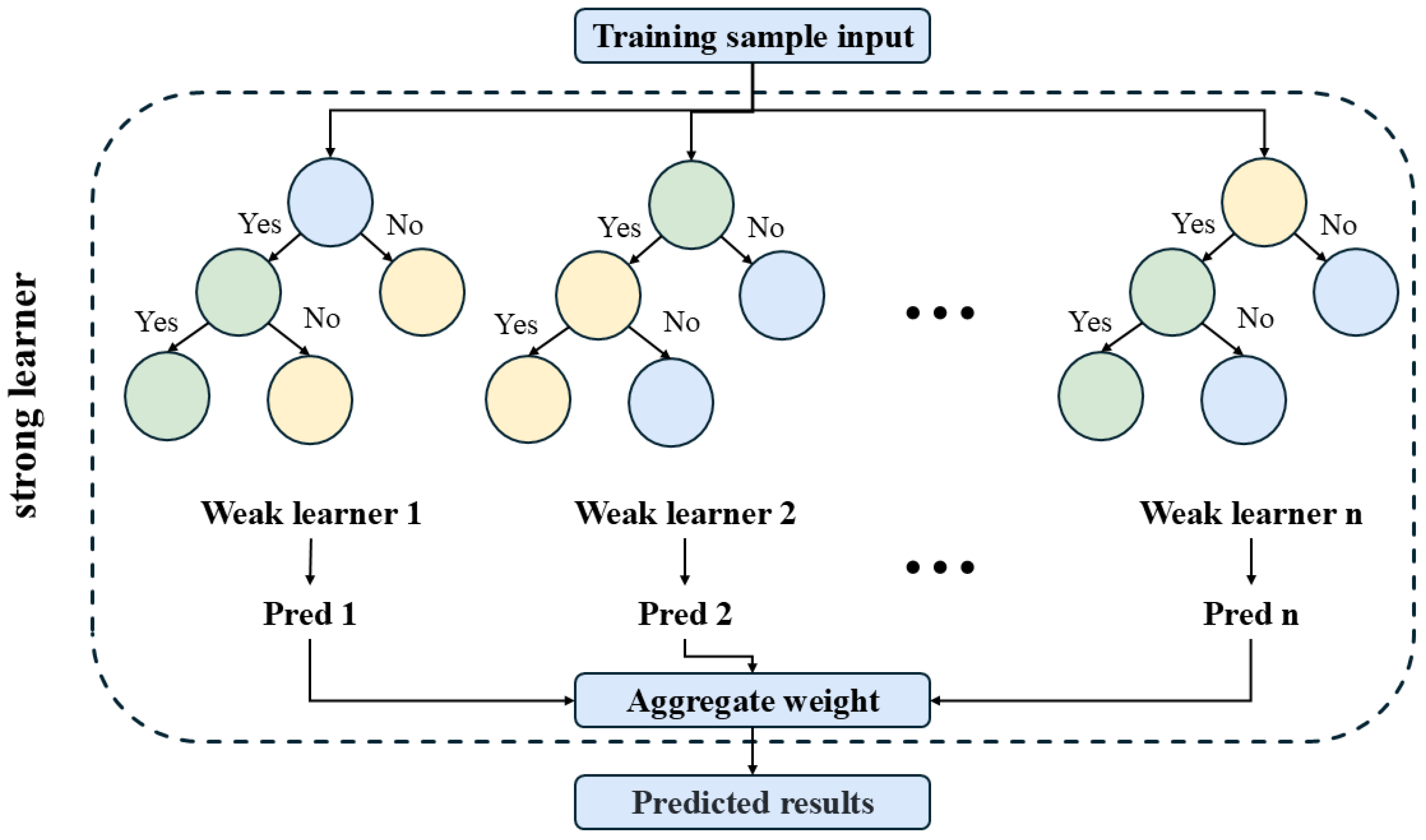
2.6.1. Extreme Gradient Boosting

Extreme Gradient Boosting (XGBoost) is an efficient decision tree algorithm based on gradient boosting. It introduces several innovations to the traditional Gradient Boosting Decision Tree (GBDT) framework, markedly improving model performance and efficiency [46]. The core idea of XGBoost is to enhance the predictive capability of the model by incrementally optimizing the loss function. As a forward additive model, it makes predictions by combining multiple weak learners (i.e., decision trees) into a strong learner. During the training process, each new tree aims to fit the residuals (i.e., prediction errors) between the target values and the predictions of all existing trees. By continually reducing these residuals, XGBoost gradually enhances the prediction accuracy of the entire model. Figure 2 provides a schematic of the model.

2.6.2. Back Propagation Neural Network

The Back Propagation Neural Network (BPNN) is a type of artificial neural network that employs the backpropagation learning algorithm. It generally consists of an input layer, one or more hidden layers, and an output layer. During training, the network receives input data, calculates the output, and compares it to the expected result. The difference is used to compute an error signal, which is then backpropagated through the network to update the weights. Figure 3 provides a schematic of the model.

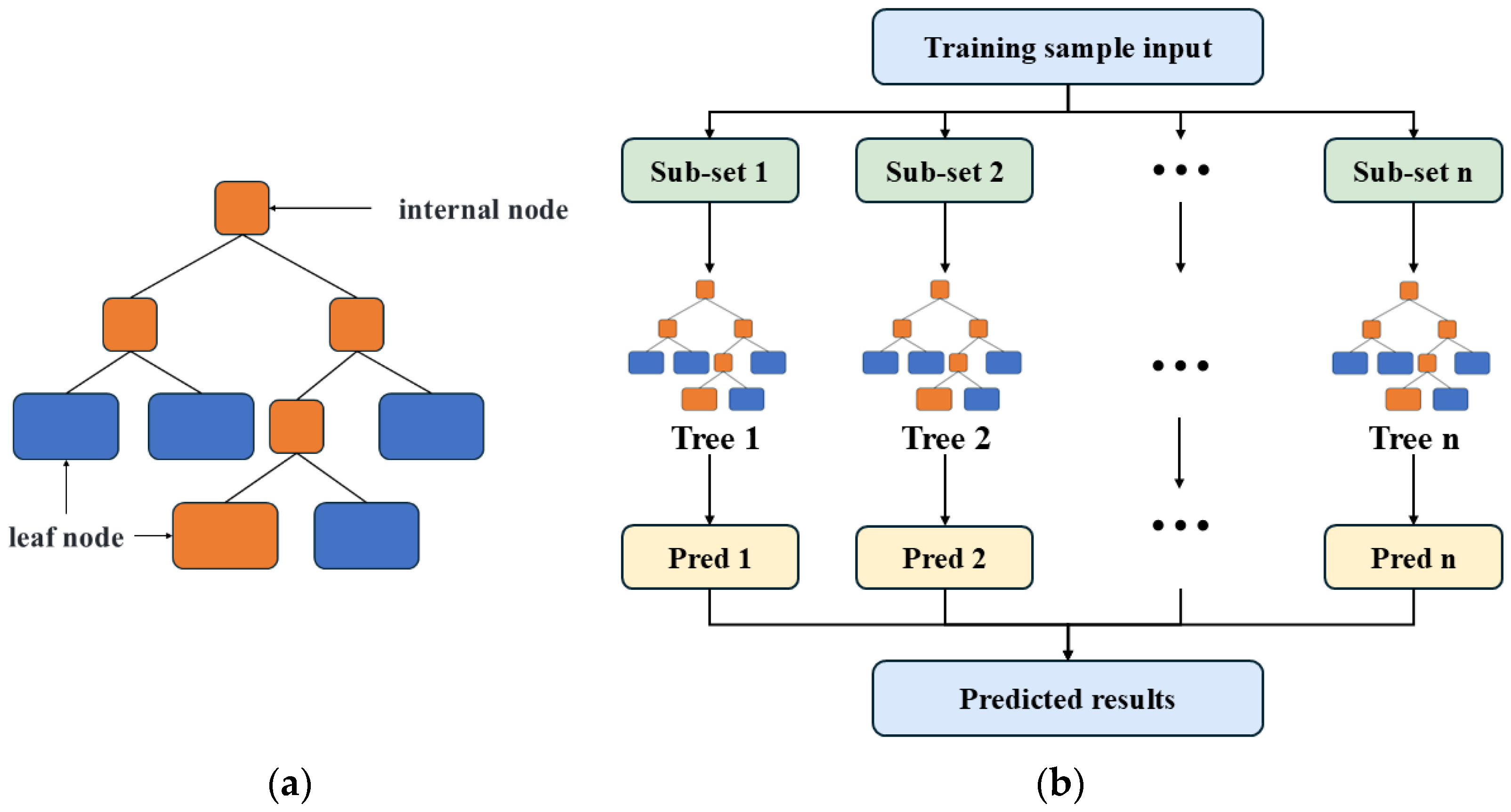
2.6.3. Random Forest

The Random Forest (RF) model is an ML algorithm based on ensemble learning and random feature selection. It improves the accuracy and robustness of the decision trees by constructing multiple decision trees and combining their prediction results. In a Random Forest, each decision tree is trained on sub-samples randomly selected from the original dataset using bootstrap sampling. Moreover, whenever a decision tree splits a node, the algorithm randomly selects a subset of features and makes the split decision based only on those features. Through the double randomization of samples and features, RF effectively reduces the risk of overfitting that may occur with individual decision trees. For regression tasks, the final prediction is obtained by averaging the results from all decision trees, enhancing the model’s stability and accuracy. Figure 4 provides a schematic representation of the model.

2.6.4. Support Vector Regression

Support Vector Regression (SVR) is a regression analysis method based on the principles of Support Vector Machines (SVMs). The goal of SVR is to define a regression function that ensures that the prediction errors are within a predefined ε (tolerance) range without penalty while simultaneously minimizing the complexity of the model. This helps ensure that the model not only fits the training data well but also maintains good generalization ability. When dealing with nonlinear relationships, SVR uses a kernel function to map the data into a higher-dimensional space [47], where linear fitting can be applied to address the nonlinear regression problem.

2.7. Settings of Model Parameter

In ML, hyperparameters play a crucial role in the performance of models. To optimize the performance of each model, it is necessary to determine the optimal hyperparameter settings through iterative experiments that evaluate prediction errors between predicted and observed values. This study employed a cross-validated grid search to identify optimal parameters for enhancing model performance; a summary of the hyperparameter settings for the four models is presented in

Table 3. ML training parameters.

Model	Parameters	PCC	GRA	MI	SR
XGBoost	learning_rate	0.1	0.01	0.01	0.01
	max_depth	11	5	9	9
	n_estimators	100	500	300	200
	subsample	0.6	0.6	1.0	0.6
	colsample_bytree	0.8	0.8	0.8	0.9
BPNN	hidden_layer_sizes	(50)	(50, 50)	(50)	(50, 50)
	activation	identity	relu	identity	tanh
	solver	lbfgs	lbfgs	lbfgs	adam
	alpha	0.0001	0.0001	0.0001	0.01
RF	n_estimators	100	200	100	100
	min_samples_split	4	5	10	5
	min_samples_leaf	2	4	2	4
	max_depth	10	20	10	20
SVR	C	10	10	10	0.1
	kernel	rbf	rbf	rbf	linear
	epsilon	0.2	0.2	0.2	0.1

.

2.8. Evaluation Metrics

After using ML models for predictions, it is essential to evaluate their performance to analyze their accuracy and practicality. This study employed commonly used evaluation metrics, including root mean square error (RMSE), Mean Absolute Error (MAE), Nash–Sutcliffe Efficiency (NSE), and Coefficient of Determination (R²), to assess the performance of various ML models. The formulas for these evaluation metrics are as follows [19]:

$$RMSE=\sqrt{{\displaystyle \frac{1}{n}}{\displaystyle \sum _{i=1}^n{(O_i-S_i)}^2}},$$

(4)

$$MAE={\displaystyle \frac{1}{n}}{\displaystyle \sum _{i=1}^n\left|O_i-S_i\right|},$$

(5)

$$NSE=1-{\displaystyle \frac{{\displaystyle \sum _{i=1}^n{\left(O_i-S_i\right)}^2}}{{\displaystyle \sum _{i=1}^n{\left(O_i-\overline{O}\right)}^2}}},$$

(6)

$$R^2={\left[{\displaystyle \frac{{\displaystyle \sum _{i=1}^n(O_i-\overline{O})(S_i-\overline{S})}}{\sqrt{{\displaystyle \sum _{i=1}^n{(O_i-\overline{O})}^2}}\sqrt{{\displaystyle \sum _{i=1}^n{(S_i-\overline{S})}^2}}}}\right]}^2,$$

(7)

where O_i and S_i represent the observed and predicted values of the river ice break-up date, respectively; $\overline{O}$ and $\overline{S}$ are the mean values of the observed and simulated data; n is the length of the sequence; and SD_O and SD_S are the standard deviations of the observed and predicted values, respectively. These statistics can be defined using the following formulas:

$$S{D}_O=\sqrt{{\displaystyle \frac{{\displaystyle \sum _{i=1}^n{(O_i-\overline{O})}^2}}{n}}}$$

(8)

$$S{D}_S=\sqrt{{\displaystyle \frac{{\displaystyle \sum _{i=1}^n{(S_i-\overline{S})}^2}}{n}}}$$

(9)

To visually represent the performance of different ML models, a Taylor diagram offers an effective visualization method. This diagram integrates the correlation coefficient (R), standard deviation (SD), and centered root mean square error (CRMSE) into a polar coordinate system using the cosine theorem. By plotting the R, SD, and CRMSE of the simulated values against the observed values on the Taylor diagram, model performance can be represented as points. The relationships between these statistics are defined using the following formulas:

$$CRMS{E}^2=S{D_O}^2+S{D_S}^2-2S{D}_{O}S{D}_{S}R$$

(10)

Among them, the centered CRMSE between observed and predicted values can be defined using the following equation:

$$CRMSE=\sqrt{{\displaystyle \frac{1}{n}}{\displaystyle \sum _{i=1}^n{\left[(O_i-\overline{O})-(S_i-\overline{S})\right]}^2}}$$

(11)

The Taylor diagram can intuitively quantify the correlation between simulated and observed points. The Taylor Skill Score (TSS) is a numerical summary of the Taylor diagram and reflects a comprehensive measure of simulation skill. The calculation formula for the Taylor Skill Score is as follows:

$$TSS={\displaystyle \frac{4(1+R{)}^4}{{(\frac{S{D}_S}{S{D}_O}+\frac{S{D}_O}{S{D}_S})}^2{(1+R_0)}^4}}$$

(12)

where TSS represents the Taylor Skill Score, where a higher score indicates better model performance. R₀ is the maximum R between the predicted and observed river ice break-up date.

2.9. Model Simulations

The framework for predicting the river ice break-up date comprises four key steps: data collection and preprocessing, ML model construction, model simulation, and model evaluation. This framework efficiently processes input data, constructs appropriate prediction models, and systematically evaluates their performance to enhance the accuracy of river ice break-up date predictions.

Firstly, based on previous research [24,40], variables that could trigger IJFs were identified and collected. The collected data were subsequently normalized using Min-Max normalization to eliminate the impact of differing units and scales on model training. Different feature selection methods were used to filter out the feature combinations that have a significant impact on IJFs. These selected features were then fed into different models, which were trained using the data from the training set to learn the relationship between the features and the river ice break-up date. Grid search was employed to explore all possible hyperparameter combinations to find the best configuration. The performance of the models on the test set is evaluated using a variety of evaluation metrics (MAE, RMSE, R², NSE, and TSS) to determine the model’s ability to generalize to unseen data. Figure 5 outlines the research framework.

3. Results and Analysis

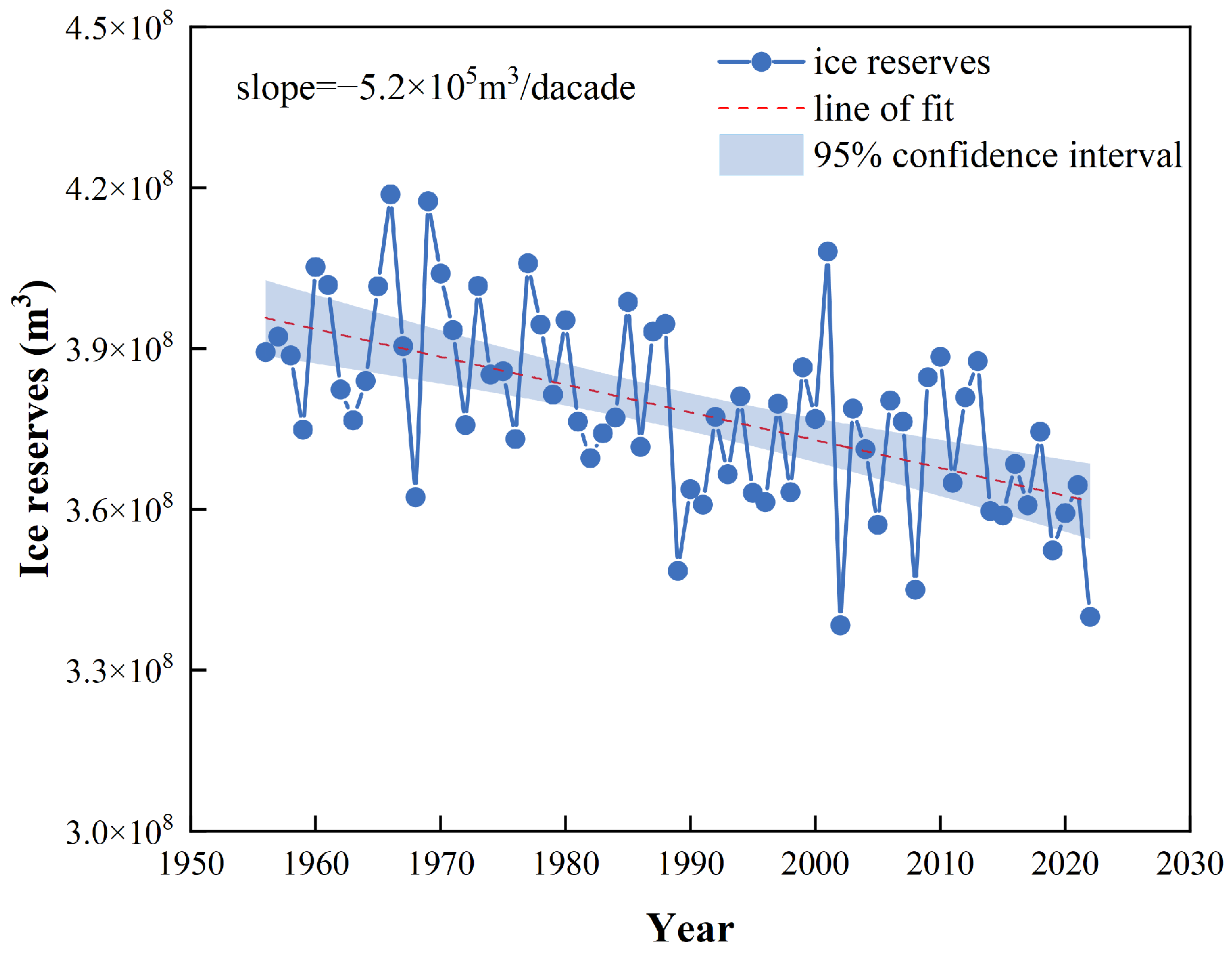
3.1. Ice Conditions Change

Figure 6 shows that the average ice reserves in the upper reaches of the Heilongjiang River from 1956 to 2022 were 3.79 × 10⁸ m³, with maximum and minimum ice reserves recorded in 1966 and 2002, respectively, representing a difference of 1 × 10⁸ m³. The Mann–Kendall test produced a Z-value of −4.89, suggesting a significant downward trend with a rate of change of 5.2 × 10⁵ m³ per decade (p < 0.05).

To simplify the calculations and investigate the influence of ice reserves on the river ice break-up date, we analyzed the effects of river sections on the break-up date using MI, PCC, and GRA methods. The results indicate that, among the upper Heilongjiang River sections, the ice reserves in the segment from Oupu to Heihe have the most significant impact on the river ice break-up date at the Heihe section, with correlation coefficients, grey relational degrees, and MI values of 0.480, 0.479, and 0.176, respectively. Consequently, we chose the ice reserves in the section from Oupu to Heihe as a candidate feature for predicting the river ice break-up date at the Heihe section.

3.2. Correlation Analysis

In this study, twelve candidate predictive factors were identified as potential input features. The significance of the relationship between the river opening date and these candidate input features was quantified using MI, PCC, SR, and GRA.

Table 4. Feature selection results.

Study Area	PCC	GRA	MI	SR
Heihe section	X1, X2, X3, X4, X6, X8, X11	X1, X2, X3, X4, X6, X11	X1, X2, X3, X4	X1, X3, X5, X7, X9, X11

presents the final results after feature selection, while Figure 7 shows the detailed results.

In the feature selection based on PCC, the significance levels of X₅, X₇, X₉, X₁₀, and X₁₂ were greater than 0.05, so these features were excluded from further analysis. X₁ and X₃ exhibited significant negative correlations with the river ice break-up date (p < 0.05), with correlation coefficients of −0.69 and −0.59, indicating that the river ice break-up date advances as accumulated temperature during the break-up period and average temperature before river ice break-up increase. On the other hand, X₂, X₄, X₆, X₈, and X₁₁ exhibited significant positive correlations with the river ice break-up date (p < 0.05), with correlation coefficients of 0.65, 0.48, 0.35, 0.29, and 0.41, respectively. The increase in these positively correlated characteristic values will lead to a delay in the river’s ice break-up date that year. This is consistent with the findings of Magnuson et al. on the relationship between climate change and river ice break-up dates [48,49,50,51], further confirming the impact of climate change on river ice conditions.

In the GRA-based feature selection process, a threshold of 0.3 was set for screening, which excluded candidate features X₅, X₇, X₈, X₉, X₁₀, and X₁₂. Additionally, in the MI feature selection, the significance levels of X₁ to X₄ were less than 0.05 based on permutation tests, so these features were selected for forecasting the river ice break-up date. In the Python 3.8 environment, SR was conducted using the ordinary least squares (OLS) method from the statsmodels library, with significance levels for introducing (α) and removing (β) variables set to 0.4. The analysis results indicated that factors X₁, X₁₁, X₃, X₇, X₉, and X₅ were sequentially included in the model. However, after introducing new variables, the influence of X₂ became non-significant and was subsequently excluded.

In the study at the Heihe section, four feature selection methods consistently identified “Accumulated temperature during the break-up period” (X₁) and “Average temperature before river ice break-up” (X₃) as key features, with strong predictive power for forecasting the river ice break-up date. Relatively, precipitation has a minor effect on the river ice break-up date, particularly “precipitation during the river opening period” (X₁₀), which was not selected in any of the four feature selection methods. The results suggest that different feature selection methods screen the data through different criteria, objectives, and algorithms and that these methods may focus on different characteristics during the selection process, and therefore, their final screening results may differ.

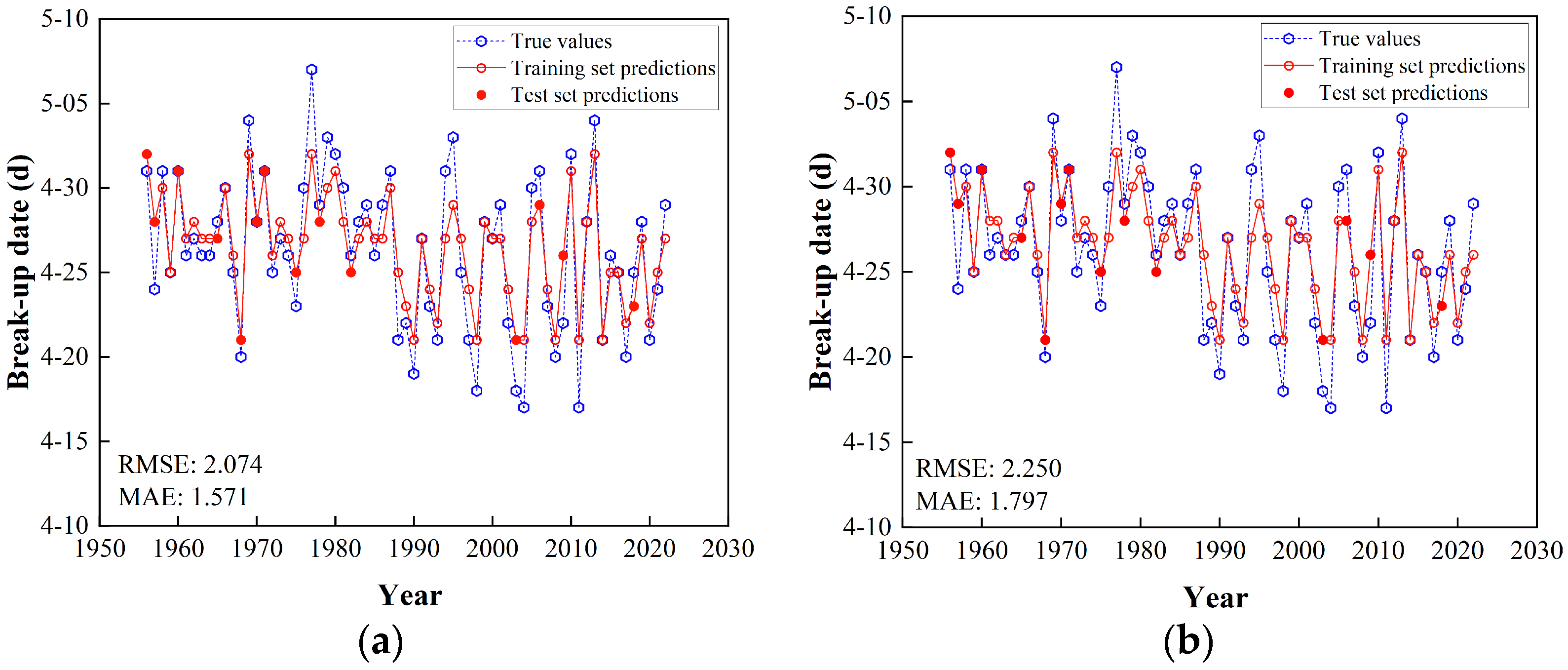
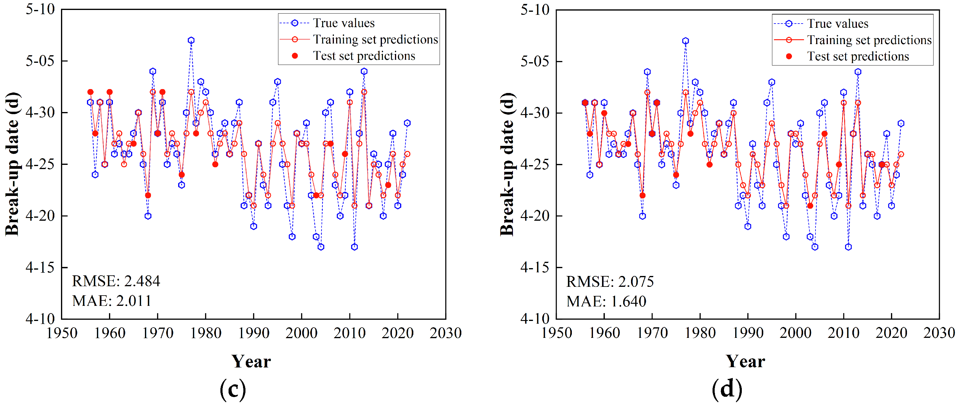
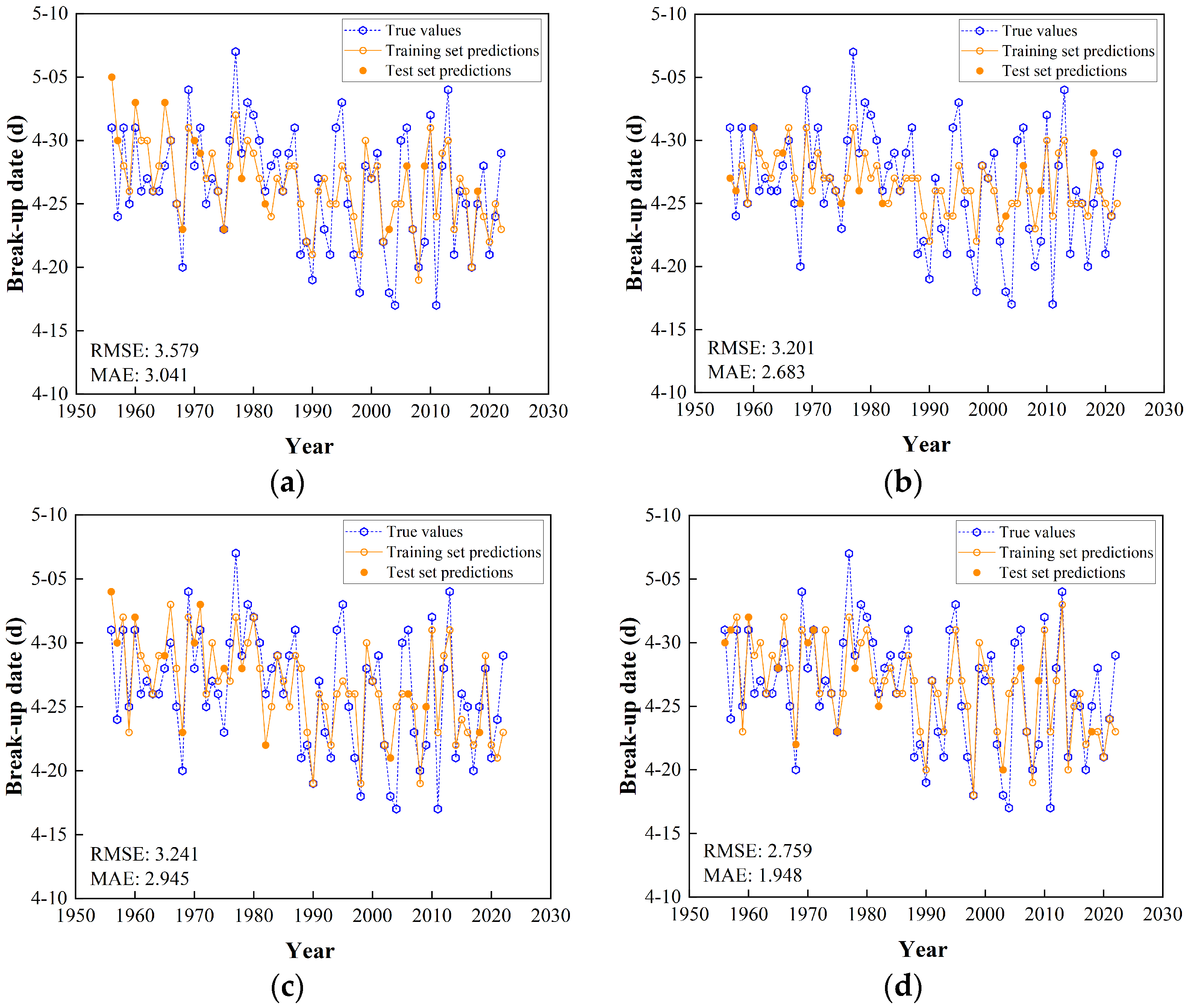
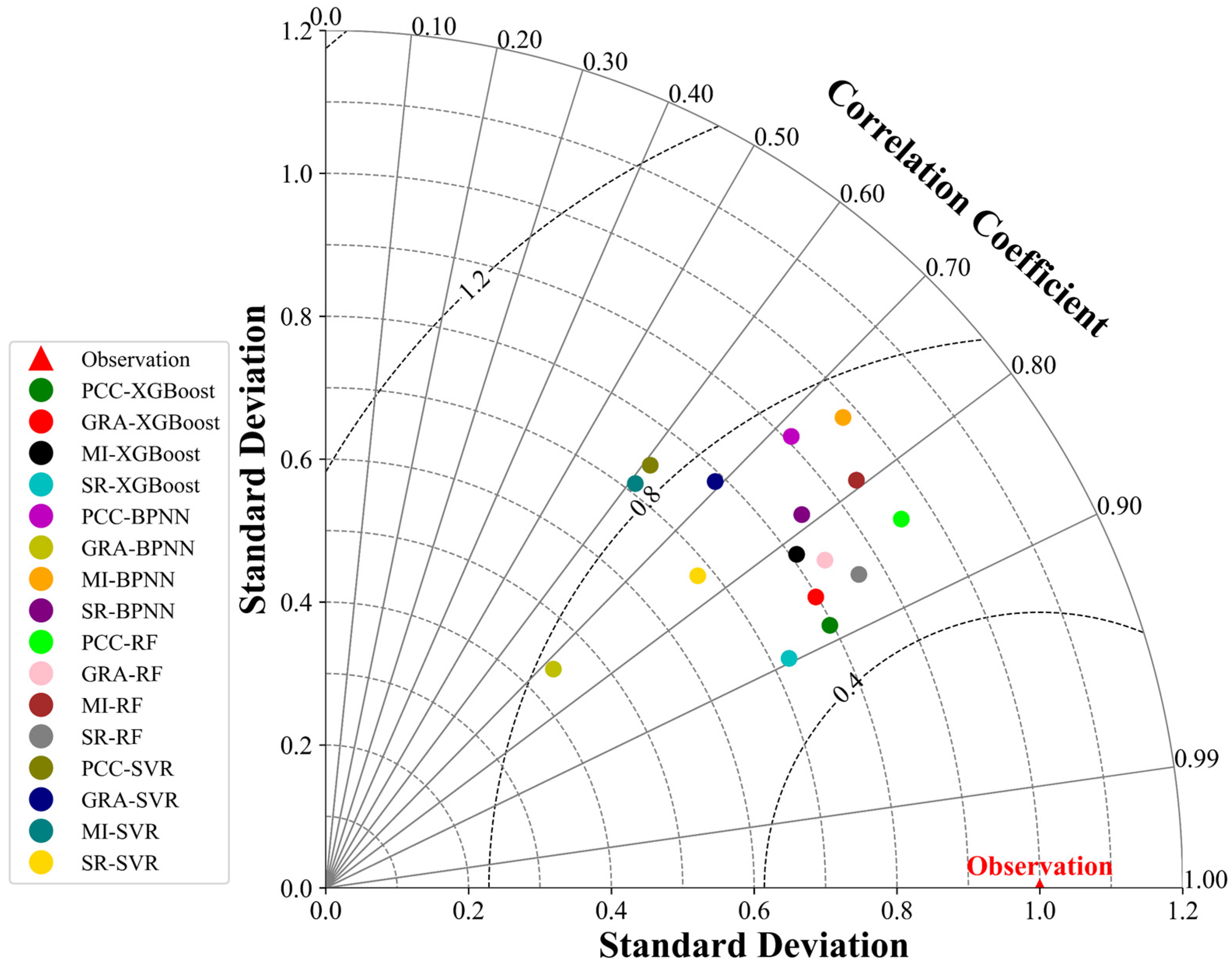
3.3. Results of Predicting River Ice Break-Up Dates

This study imports the features selected by different feature selection methods to different ML models for making predictions. Figure 8, Figure 9, Figure 10, and Figure 11 show different ML model predictions based on different feature selection methods, respectively. In the figures, the blue dashed line represents the actual river ice break-up dates, while the solid line with hollow markers indicates the predictions for the training set, and the solid markers represent the predictions for the test set.

Between 1956 and 2022, the earliest and latest river ice break-up dates at the Heihe section occurred on 15 April 2004 and 5 May 1977, respectively, resulting in a 20-day interval. The Mann–Kendall test yielded a Z-value of −2.14, indicating a significant trend of advancement in the river ice break-up date at the Heihe section, with a rate of change of 0.682 days per decade (p < 0.05). Over the 67-year period, the river ice break-up date advanced by 4.57 days in total. The Mann–Kendall mutation test revealed that the river ice break-up date at the Heihe section experienced significant changes in 1969, 2005, 2011, and 2014.

From

Table 5. Model performance on training and test sets.

Model	Methods	Training Set					Test Set
		RMSE	MAE	R2	NSE	TSS	RMSE	MAE	R2	NSE	TSS
XGBoost	PCC	1.950	1.537	0.907	0.823	0.848	2.074	1.571	0.784	0.756	0.950
	GRA	1.998	1.553	0.895	0.814	0.836	2.250	1.797	0.740	0.712	0.901
	MI	2.185	1.722	0.863	0.778	0.783	2.484	2.011	0.666	0.649	0.822
	SR	2.206	1.782	0.883	0.774	0.769	2.075	1.640	0.803	0.755	0.923
BPNN	PCC	3.140	2.645	0.549	0.539	0.521	3.579	3.041	0.514	0.272	0.682
	GRA	3.412	2.807	0.523	0.458	0.358	3.201	2.683	0.520	0.418	0.379
	MI	3.041	2.402	0.571	0.570	0.615	3.241	2.945	0.547	0.403	0.724
	SR	2.850	2.206	0.623	0.622	0.655	2.759	1.948	0.620	0.567	0.785
RF	PCC	1.475	1.116	0.914	0.898	0.974	2.442	2.038	0.708	0.661	0.907
	GRA	1.993	1.577	0.827	0.815	0.871	2.445	2.041	0.699	0.660	0.892
	MI	2.103	1.689	0.806	0.794	0.885	2.690	2.232	0.628	0.589	0.813
	SR	2.243	1.740	0.787	0.766	0.799	2.283	1.871	0.743	0.704	0.932
SVR	PCC	3.369	2.557	0.484	0.472	0.436	3.179	2.738	0.468	0.426	0.585
	GRA	3.242	2.309	0.537	0.511	0.476	2.969	2.451	0.511	0.499	0.647
	MI	3.413	2.602	0.476	0.458	0.412	3.180	2.736	0.441	0.425	0.543
	SR	3.121	2.560	0.631	0.547	0.461	2.813	2.325	0.551	0.550	0.680

, we observe that different combinations of models and feature selection methods have a significant impact on the prediction performance. Overall, there are notable differences in the prediction performance of the models when different feature selection methods are used. Taking RMSE and MAE as examples, under different feature selection methods, the RMSE and MAE values of each model fluctuate, indicating that feature selection has an important impact on model prediction accuracy. Furthermore, specific to each model, we observe that the XGBoost model generally exhibits superior prediction performance. In particular, PCC-XGBoost achieves the best prediction accuracy and model fit. In addition, SR-BPNN exhibits relatively good performance. The BPNN’s R² and NSE values improved when combined with SR, indicating that SR optimized the feature set of the RF to a certain extent, thus enhancing its predictive ability and model fit. The RF model, on the other hand, exhibits relatively stable predictive performance, with its RMSE, MAE, R², and NSE values remaining within a relatively stable range regardless of which feature selection method is used. Regarding the SVR model, its prediction performance tends to be relatively weaker across most feature selection methods; its R² and NSE values also increase under the SR method, indicating that SR has also optimized the feature set of the SVR to some extent.

In summary, the impact of feature selection methods on model performance is significant. Different feature selection methods can result in significant differences in model prediction accuracy and fit. Therefore, it is crucial to choose an appropriate feature selection method when performing model training. For a particular model and dataset, it may be necessary to experimentally compare the performance of different feature selection methods to select the most suitable feature set and model combination.

To comprehensively evaluate the prediction results of river ice break-up dates, this study employed five metrics: RMSE, MAE, R², NSE, and TSS. Given that different ML models exhibit varying performances on these metrics, we utilized Taylor diagrams as a visual representation of model performance. The Taylor diagram integrates the correlation coefficient, standard deviation, and CRMSE within a polar coordinate system, thereby illustrating the agreement between predicted and observed ice break-up dates. In the Taylor diagram, the radial distance from the origin to the predicted point represents the standard deviation. The cosine of the azimuthal angle signifies the correlation coefficient between the predicted and observed values; hence, an angle nearer to the origin direction indicates a correlation coefficient closer to +1, suggesting a stronger linear relationship between the two sets of values. The CRMSE is depicted by the distance between the predicted and observed points, with a shorter distance implying that the model’s predictions are more consistent with the observed data, reflecting better model performance.

The Taylor diagram results are shown in Figure 12. Notably, when the same model is applied with different feature selection methods, there are discernible variations in the predictions of the river ice break-up dates. Similarly, when the same feature selection method is employed, significant performance disparities arise among different models. The distribution within the Taylor diagram is quite scattered, with notable differences. The correlation coefficients of the 16 model combinations range from 0.66 to 0.89. Furthermore, the worst-performing model combination is GRA-BPNN, situated farthest from the observation point, with a TSS of 0.379. In contrast, the best-performing combination is PCC-XGBoost, positioned closer to the observation point, boasting a TSS of 0.950. This indicates that PCC-XGBoost surpasses the other combinations in terms of prediction accuracy. Therefore, PCC-XGBoost was selected as the prediction model for the Heihe section.

Based on the Standard for hydrological information and hydrological forecasting, for ice forecasts with a lead time of 6 to 10 days, a maximum permissible error of 3 days is established. Forecasts with an absolute error of less than 3 days are considered acceptable. The PCC-XGBoost model has a qualification rate of 85.71%, meeting the standard for first-class forecasting.

4. Discussion

The study results indicate a clear downward trend in the ice reserves volume in the upper reaches of the Heilongjiang River during the study period. This finding was confirmed using the Mann–Kendall test (Z = −4.89, p < 0.05), with a reduction of 5.2 × 10⁵ cubic meters of ice reserves per decade. These findings are consistent with the global trend of decreasing ice masses due to climate warming [52]. Furthermore, methods such as PCC, GRA, and MI indicate that the ice reserve volume from Oupu to Heihe impacts the ice break-up date at the Heihe section. This supports previous studies suggesting that ice reserves are a key climatic factor that can provide valuable information for predicting the ice break-up date [53,54]. All four feature selection methods consistently identified the accumulated temperature during the ice break-up period and the average temperature before the ice break-up as key factors influencing the break-up date. The rise in both accumulated temperature during the break-up period and the average temperature before the break-up tends to lead to an earlier ice break-up. This further reinforces the importance of climatic factors in determining the river ice break-up date [55,56]. Ice break-up in the study area has significantly advanced, with an average advancement of 0.682 days per decade. The observed trend of earlier ice break-ups is likely a direct result of warming temperatures in the region, suggesting that climate change is accelerating the ice break-up date of the Heilongjiang River’s Heihe section.

During the model development phase, input selection is often an overlooked key task. As shown in Table 5, a comparative analysis of different ML models reveals that feature selection has a significant impact on model performance. However, the best feature selection method varies depending on the structure of the ML model. This difference highlights the point that a “one-size-fits-all” feature engineering approach cannot optimize the performance of specific model structures. The four feature selection methods in this study are model-agnostic, aiming to identify predictive features independently of the underlying ML algorithm’s structure. The best-performing model is PCC-XGBoost, with a prediction accuracy of 85.71%. Compared with methods proposed in the existing literature [16], the prediction accuracy improves by 13.71%. XGBoost is a powerful ensemble learning algorithm based on gradient boosting that is known for effectively handling nonlinear relationships. It outperforms other ML algorithms in prediction because it minimizes a regularized objective function by iteratively adding decision trees that correct residuals from previous iterations [57,58]. XGBoost’s performance varies markedly across feature selection methods, with optimal results depending on scenario-specific input parameters. This aligns with the observations of Hussain and Khan [59]. XGBoost may overfit in imbalanced or extreme event data, and careful adjustment of regularization parameters is required [60]. The performance of BPNN is unstable. Although the best model can be obtained by iteratively adjusting parameters [61], BPNN has limited generalization ability in extreme climate event prediction, primarily due to the insufficient coverage of extreme scenarios in the training data rather than the network architecture itself [62,63]. This issue has also been confirmed by Dai et al. [64] through multiple experiments. As the model is trained, RF performs better than SVR and BPNN. Tyralis et al. [65] confirmed that RF has better stability and prediction performance compared with other ML models. However, RF is sensitive to noise or irrelevant features, which may reduce its generalization performance. Despite these limitations, ensemble and hybrid models generally improve prediction performance compared with independent ML methods, as clearly confirmed in the literature [35]. Compared with other machine learning models, SVR performs poorly in this study. Despite systematic hyperparameter tuning of SVR through grid search, its prediction accuracy remains significantly lower than that of other models. This phenomenon may be due to the highly non-stationary and asymmetric nonlinear relationships between the climate variables involved in the study, while SVR relies on kernel functions to map data into high-dimensional space for linear separation. Although theoretically, the RBF kernel can handle complex nonlinearity, its performance in practice is limited by challenges such as insufficient sample size and high feature dimensions [66]. When the training data fail to adequately cover the distribution range of extreme events, SVR struggles to learn a robust decision boundary from the limited samples.

In addition, this study has several limitations that need to be addressed and explored in future research. The results of the current ice reserve calculations are influenced by the accuracy of the freezing degree-day model and the precision of river freezing area calculations. In future research, we plan to utilize satellite remote sensing data to enhance the accuracy of ice reserve calculations. In ML, the quality of the data directly affects the model’s performance and predictive ability. If the data contain noise, missing values, or outliers, the accuracy and robustness of the model will be compromised. In this study, although we made efforts to collect a broad dataset for training the ML model, the insufficient precision of the data may negatively impact the model’s predictive performance. Additionally, we observed that significant errors in the meteorological information of the input data typically lead to decreased model prediction accuracy. This could be because the meteorological information serves as a key input feature for predicting the river ice break-up date, and its accuracy is directly related to the model’s predictive performance. With the continuous expansion of future datasets and the emergence of high-precision data, we expect the model’s accuracy to improve significantly, leading to more reliable predictions. Given the complexity involved in the formation of the IJF, further studies could incorporate additional feature engineering or consider integrating feature engineering with model architecture optimization during preprocessing. We will also focus on improving the interpretability of the model. This includes optimizing the selection of features and indicators, as well as applying the SHAP method to analyze the impact of different features on the river ice break-up date.

5. Conclusions

This study analysed and calculated river ice break-up dates and ice reserves in upper Heilongjiang from 1956 to 2022. In addition, key features of the break-up dates in the study area were screened based on multiple feature selection techniques (MI, PCC, SR, and GRA) to optimize the prediction accuracy of the ML models (XGBoost, BPNN, RF, and SVR). The results of the study show the follwoing:

• The river ice break-up date of the Heihe section of the Heilongjiang River shows an early trend, with the river ice break-up date advancing by 0.682 days every 10 years. The ice reserves in the Oupu–Heihe section in the upper reaches of the Heilongjiang River have the most significant impact on the river ice break-up date in the Heihe section. The correlation coefficient, grey relational degree, and mutual information value were 0.480, 0.479, and 0.176, respectively.
• The different feature sets obtained for feature selection using PCC, MI, GRA, and SR reflect the different data characteristics that these methods focus on. Accumulated temperature during the break-up period and average temperature before river ice break-up were considered to have a significant effect on the opening of the river for a wide range of criteria, with abrupt temperature changes being a key factor affecting the timing of the opening of the river.
• The best feature selection method varies depending on the structure of the ML model. By comparing 16 different combinations, PCC-XGBoost resulted in the smallest bias, achieving a prediction accuracy of 85.71%. According to the Standard for Hydrological Information and Hydrological Forecasting, this is classified as a first-class solution and can be used for river opening date prediction.

References

1. Lindenschmidt, K.-E.; Rokaya, P. A stochastic hydraulic modelling approach to determining the probable maximum staging of ice-jam floods. J. Environ. Inform. 2019, 34, 45–54. [Google Scholar] [CrossRef]
2. Hicks, F.; Beltaos, S. River Ice. In Cold Region Atmospheric and Hydrologic Studies. The Mackenzie GEWEX Experience; Woo, M., Ed.; Springer: Berlin/Heidelberg, Germany, 2008; pp. 281–305. [Google Scholar] [CrossRef]
3. Rokaya, P.; Budhathoki, S.; Lindenschmidt, K.-E. Ice-jam flood research: A scoping review. Nat. Hazards 2018, 94, 1439–1457. [Google Scholar] [CrossRef]
4. Cunderlik, J.M.; Ouarda, T.B.M.J. Trends in the timing and magnitude of floods in Canada. J. Hydrol. 2009, 375, 471–480. [Google Scholar] [CrossRef]
5. Ghoreishi, M.; Lindenschmidt, K.-E. Unlocking effective ice-jam risk management: Insights from agent-based modeling and comparative analysis of social theories in Fort McMurray, Canada. Environ. Sci. Policy 2024, 157, 103731. [Google Scholar] [CrossRef]
6. Pagneux, E.; Gísladóttir, G.; Jónsdóttir, S. Public perception of flood hazard and flood risk in Iceland: A case study in a watershed prone to ice-jam floods. Nat. Hazards 2011, 58, 269–287. [Google Scholar] [CrossRef]
7. Das, A.; Lindenschmidt, K.-E. Current status and advancement suggestions of ice-jam flood hazard and risk assessment. Environ. Rev. 2020, 28, 373–379. [Google Scholar] [CrossRef]
8. Das, A.; Budhathoki, S.; Lindenschmidt, K.-E. Development of an ice-jam flood forecasting modelling framework for freeze-up/winter breakup. Hydrol. Res. 2023, 54, 648–662. [Google Scholar] [CrossRef]
9. Barrette, P.D.; Khan, A.A.; Lindenschmidt, K.-E. A glimpse at twenty-five hydraulic models for river ice. In Proceedings of the 27th IAHR International Symposium on Ice, Gdańsk, Poland, 9–13 June 2024; Available online: https://www.iahr.org/library/infor?pid=30349 (accessed on 20 May 2023).
10. Lindenschmidt, K.-E. RIVICE—A Non-Proprietary, Open-Source, One-Dimensional River-Ice Model. Water 2017, 9, 314. [Google Scholar] [CrossRef]
11. Fu, H.; Guo, X.; Yang, K.; Wang, T.; Guo, Y. Ice accumulation and thickness distribution before inverted siphon. J. Hydrodyn. 2017, 29, 61–67. [Google Scholar] [CrossRef]
12. Carson, R.; Beltaos, S.; Groeneveld, J.; Healy, D.; She, Y.; Malenchak, J.; Morris, M.; Saucet, J.-P.; Kolerski, T.; Shen, H.T. Comparative testing of numerical models of river ice jams. Can. J. Civ. Eng. 2011, 38, 669–678. [Google Scholar] [CrossRef]
13. Beltaos, S. Numerical modelling of ice-jam flooding on the Peace-Athabasca delta. Hydrol. Process. 2003, 17, 3685–3702. [Google Scholar] [CrossRef]
14. Ladouceur, J.-R.; Morse, B.; Lindenschmidt, K.-E. A comprehensive method to estimate flood levels of rivers subject to ice jams: A case study of the Chaudière River, Québec, Canada. Hydrol. Res. 2023, 54, 995–1016. [Google Scholar] [CrossRef]
15. Beltaos, S.; Burrell, B.C. Hydrotechnical advances in Canadian river ice science and engineering during the past 35 years. Can. J. Civ. Eng. 2015, 42, 583–591. [Google Scholar] [CrossRef]
16. Lei, Q.; Zhang, D.; Li, J. Discussion on the ice breakup forecasting and analysis method at Jiayin station, Heilongjiang. Heilongjiang Hydr. Sci. Technol. 2010, 39, 16–17. (In Chinese) [Google Scholar]
17. Lindenschmidt, K.-E.; Rokaya, P.; Das, A.; Li, Z.; Richard, D. A novel stochastic modelling approach for operational real-time ice-jam flood forecasting. J. Hydrol. 2019, 575, 381–394. [Google Scholar] [CrossRef]
18. Smith, J.D.; Lamontagne, J.R.; Jasek, M. Considering uncertainty of historical ice jam flood records in a Bayesian frequency analysis for the Peace-Athabasca Delta. Water Resour. Res. 2024, 60, e2022WR034377. [Google Scholar] [CrossRef]
19. Liu, M.; Wang, Y.; Xing, Z.; Wang, X.; Fu, Q. Study on forecasting break-up date of river ice in Heilongjiang Province based on LSTM and CEEMDAN. Water 2023, 15, 496. [Google Scholar] [CrossRef]
20. Shevnina, E.V.; Solov’eva, Z.S. Long-term variability and methods of forecasting dates of ice break-up in the mouth area of the Ob and Yenisei rivers. Russ. Meteorol. Hydrol. 2008, 33, 458–465. [Google Scholar] [CrossRef]
21. Madaeni, F.; Chokmani, K.; Lhissou, R.; Gauthier, Y.; Tolszczuk-Leclerc, S. Convolutional neural network and long short-term memory models for ice-jam predictions. Cryosphere 2022, 16, 1447–1468. [Google Scholar] [CrossRef]
22. Kalke, H.; Loewen, M. Support vector machine learning applied to digital images of river ice conditions. Cold Reg. Sci. Technol. 2018, 155, 225–236. [Google Scholar] [CrossRef]
23. Tom, M.; Prabha, R.; Wu, T.; Baltsavias, E.; Leal-Taixé, L.; Schindler, K. Ice monitoring in Swiss lakes from optical satellites and webcams using machine learning. Remote Sens. 2020, 12, 3555. [Google Scholar] [CrossRef]
24. Chen, S.; Ji, H. Fuzzy optimization neural network approach for ice forecast in the Inner Mongolia reach of the Yellow River. Hydrol. Sci. J. 2005, 50, 319–330. [Google Scholar] [CrossRef]
25. Ge, Q.; Wang, J.; Liu, C.; Wang, X.; Deng, Y.; Li, J. Integrating feature selection with machine learning for accurate reservoir landslide displacement prediction. Water 2024, 16, 2152. [Google Scholar] [CrossRef]
26. Paulson, N.H.; Kubal, J.; Ward, L.; Saxena, S.; Lu, W.; Babinec, S.J. Feature engineering for machine learning enabled early prediction of battery lifetime. J. Power Sources 2022, 527, 231127. [Google Scholar] [CrossRef]
27. Chicco, D.; Oneto, L.; Tavazzi, E. Eleven quick tips for data cleaning and feature engineering. PLoS Comput. Biol. 2022, 18, e1010718. [Google Scholar] [CrossRef]
28. Diebold, F.X.; Göbel, M.; Coulombe, P.G. Assessing and comparing fixed-target forecasts of Arctic sea ice: Glide charts for feature-engineered linear regression and machine learning models. Energy Econ. 2023, 124, 106833. [Google Scholar] [CrossRef]
29. Nichol, J.J.; Peterson, M.G.; Peterson, K.J.; Fricke, G.M.; Moses, M.E. Machine learning feature analysis illuminates disparity between E3SM climate models and observed climate change. J. Comput. Appl. Math. 2021, 395, 113451. [Google Scholar] [CrossRef]
30. Verdonck, T.; Baesens, B.; Óskarsdóttir, M.; vanden Broucke, S. Special issue on feature engineering editorial. Mach. Learn. 2024, 113, 3917–3928. [Google Scholar] [CrossRef]
31. Ji, H.; Zhang, A.; Gao, R.; Zhang, B.; Xu, J. Application of the break-up date prediction model in the Inner Mongolia Reach of the Yellow River. Adv. Sci. Technol. Water Res. 2012, 32, 42–45. [Google Scholar]
32. Li, C.; Guo, X.; Wang, Z. Determination on forecast factor of artificial intelligence ice-forecast. Water Resour. Hydropower Eng. 2012, 43, 9–13. (In Chinese) [Google Scholar] [CrossRef]
33. Rokaya, P.; Budhathoki, S.; Lindenschmidt, K.-E. Trends in the Timing and magnitude of ice-jam floods in Canada. Sci. Rep. 2018, 8, 5834. [Google Scholar] [CrossRef] [PubMed]
34. Das, A.; Lindenschmidt, K.-E. Modelling climatic impacts on ice-jam floods: A review of current models, modelling capabilities, challenges, and future prospects. Environ. Rev. 2021, 29, 378–390. [Google Scholar] [CrossRef]
35. Salimi, A.; Ghobrial, T.; Bonakdari, H. A comprehensive review of AI-based methods used for forecasting ice jam floods occurrence, severity, timing, and location. Cold Reg. Sci. Technol. 2024, 227, 104305. [Google Scholar] [CrossRef]
36. Das, A.; Rokaya, P.; Lindenschmidt, K.-E. The impact of a bias-correction approach (delta change) applied directly to hydrological model output when modelling the severity of ice jam flooding under future climate scenarios. Clim. Change 2022, 172, 19. [Google Scholar] [CrossRef]
37. Lubiniecki, T.; Laroque, C.P.; Lindenschmidt, K.-E. Identifying ice-jam flooding events through the application of dendrogeomorphological methods. River Res. Appl. 2024, 40, 191–202. [Google Scholar] [CrossRef]
38. Huang, F.; Shen, H.T. Dam removal effect on the lower St. Regis River ice-jam floods. Can. J. Civ. Eng. 2023, 51, 215–227. [Google Scholar] [CrossRef]
39. Li, Y.; Han, H.; Sun, Y.; Xiao, X.; Liao, H.; Liu, X.; Wang, E. Risk evaluation of ice flood disaster in the upper Heilongjiang River based on catastrophe theory. Water 2023, 15, 2724. [Google Scholar] [CrossRef]
40. Wang, T.; Liu, Z.; Guo, X.; Fu, H.; Liu, W. Prediction of breakup ice jam with Artificial Neural Networks. J. Hydraul. Eng. 2017, 48, 1355–1362. (In Chinese) [Google Scholar] [CrossRef]
41. Li, M.; Yang, D.; Hou, J.; Xiao, P.; Xing, X. Distributed hydrological model of Heilongjiang River basin. J. Hydroelectr. Eng. 2021, 40, 65–75. (In Chinese) [Google Scholar]
42. Cao, W.; Xiao, D.; Li, G. How to make ice dam forecasting for Heilongjiang River. J. China Hydrol. 2014, 34, 72–76. (In Chinese) [Google Scholar]
43. Chang, Y.; Liu, X.; Zhao, X.; Shen, Y. Multi-scale analysis of runoff variability and its influencing factors in the mountainous Hutuo River Basin. J. Water Resour. Eng. 2023, 34, 59–70. (In Chinese) [Google Scholar]
44. Massie, D.D.; White, K.D.; Daly, S.F. Application of neural networks to predict ice jam occurrence. Cold Reg. Sci. Technol. 2002, 35, 115–122. [Google Scholar] [CrossRef]
45. Rafi, M.N.; Imran, M.; Nadeem, H.A.; Abbas, A.; Pervaiz, M.; Khan, W.; Ullah, S.; Hussain, S.; Saeed, Z. Comparative influence of biochar and doped biochar with Si-NPs on the growth and anti-oxidant potential of Brassica rapa L. under Cd toxicity. Silicon 2022, 14, 11699–11714. [Google Scholar] [CrossRef]
46. Friedman, J.H. Greedy function approximation: A gradient boosting machine. Ann. Stat. 2001, 29, 1189–1232. [Google Scholar] [CrossRef]
47. Cortes, C.; Vapnik, V. Support-vector networks. Mach. Learn. 1995, 20, 273–297. [Google Scholar] [CrossRef]
48. Magnuson, J.J.; Robertson, D.M.; Benson, B.J.; Wynne, R.H.; Livingstone, D.M.; Arai, T.; Assel, R.A.; Barry, R.G.; Card, V.; Kuusisto, E.; et al. Historical trends in lake and river ice cover in the Northern Hemisphere. Science 2000, 289, 1743–1746. [Google Scholar] [CrossRef]
49. Prowse, T.D.; Beltaos, S. Climatic control of river-ice hydrology: A review. Hydrol. Process. 2002, 16, 805–822. [Google Scholar] [CrossRef]
50. Ji, X.; Zhao, J. Analysis of correlation between sea ice concentration and cloudiness in the central Arctic. Acta Oceanol. Sin. 2015, 37, 92–104. (In Chinese) [Google Scholar] [CrossRef]
51. Schweiger, A.J.; Lindsay, R.W.; Vavrus, S.; Francis, J.A. Relationships between Arctic sea ice and clouds during autumn. J. Clim. 2009, 22, 4799–4810. [Google Scholar] [CrossRef]
52. Jacob, T.; Wahr, J.; Pfeffer, W.T.; Swenson, S. Recent contributions of glaciers and ice caps to sea level rise. Nature 2012, 482, 514–518. [Google Scholar] [CrossRef]
53. Prowse, T.D.; Bonsal, B.R.; Duguay, C.R.; Lacroix, M.P. River-ice break-up/freeze-up: A review of climatic drivers, historical trends and future predictions. Ann. Glaciol. 2007, 46, 443–451. [Google Scholar] [CrossRef]
54. Rokaya, P.; Morales-Marín, L.; Bonsal, B.; Wheater, H.; Lindenschmidt, K.-E. Climatic effects on ice phenology and ice-jam flooding of the Athabasca River in western Canada. Hydrol. Sci. J. 2019, 64, 1265–1278. [Google Scholar] [CrossRef]
55. Burrell, B.C.; Beltaos, S.; Turcotte, B. Effects of climate change on river-ice processes and ice jams. Int. J. River Basin Manag. 2022, 21, 421–441. [Google Scholar] [CrossRef]
56. Yang, X.; Pavelsky, T.M.; Allen, G.H. The past and future of global river ice. Nature 2020, 577, 69–73. [Google Scholar] [CrossRef]
57. Chen, T.; Guestrin, C. XGBoost: A Scalable Tree Boosting System. In Proceedings of the 22nd ACM SIGKDD International Conference on Knowledge Discovery and Data Mining (KDD ’16), San Francisco, CA, USA, 13–17 August 2016; Association for Computing Machinery: New York, NY, USA, 2016; pp. 785–794. [Google Scholar] [CrossRef]
58. Niazkar, M.; Menapace, A.; Brentan, B.; Piraei, R.; Jimenez, D.; Dhawan, P.; Righetti, M. Applications of XGBoost in water resources engineering: A systematic literature review (Dec 2018–May 2023). Environ. Model. Softw. 2024, 174, 105971. [Google Scholar] [CrossRef]
59. Hussain, D.; Khan, A.A. Machine learning techniques for monthly river flow forecasting of Hunza River, Pakistan. Earth Sci. Inform. 2020, 13, 939–949. [Google Scholar] [CrossRef]
60. Zhang, W.; Wang, H.; Lin, Y.; Jin, J.; Liu, W.; An, X. Reservoir inflow predicting model based on machine learning algorithm via multi-model fusion: A case study of Jinshuitan river basin. IET Cyber-Syst. Robot. 2021, 3, 265–277. [Google Scholar] [CrossRef]
61. Aksoy, H.; Mohammadi, M. Artificial neural network and regression models for flow velocity at sediment incipient deposition. J. Hydrol. 2016, 541, 1420–1429. [Google Scholar] [CrossRef]
62. Nielsen, M.A. Neural Networks and Deep Learning; Determination Press: San Francisco, CA, USA, 2015; Available online: http://neuralnetworksanddeeplearning.com/ (accessed on 29 December 2023).
63. Hu, H.; Zhang, J.; Li, T. A novel hybrid decompose-ensemble strategy with a VMD-BPNN approach for daily streamflow estimating. Water Resour. Manag. 2021, 35, 5119–5138. [Google Scholar] [CrossRef]
64. Dai, W.; Cai, Z. Predicting coastal urban floods using artificial neural network: The case study of Macau, China. Appl. Water Sci. 2021, 11, 161. [Google Scholar] [CrossRef]
65. Tyralis, H.; Papacharalampous, G.; Langousis, A. A Brief Review of Random Forests for Water Scientists and Practitioners and their Recent History in Water Resources. Water 2019, 11, 910. [Google Scholar] [CrossRef]
66. Deka, P.C. Support vector machine applications in the field of hydrology: A review. Appl. Soft Comput. 2014, 19, 372–386. [Google Scholar] [CrossRef]
Figure 1. The geography of the study area.
Water 17 00434 g001
Figure 2. Extreme Gradient Boosting schematic.
Water 17 00434 g002
Figure 3. Neural network schematic.
Water 17 00434 g003
Figure 4. Random Forest schematic. (a) Decision tree diagram; (b) Random Forest model structure diagram.
Water 17 00434 g004
Figure 5. Flowchart of the prediction model.
Water 17 00434 g005
Figure 6. Interannual variability of ice reserves in the upper reaches of the Heilongjiang River.
Water 17 00434 g006
Figure 7. Feature importance analysis for features X1 to X12. (a) PCC; (b) GRA; (c) MI; (d) SR.
Water 17 00434 g007
Figure 8. XGBoost model prediction results. (a) PCC; (b) GRA; (c) MI; (d) SR.
Water 17 00434 g008aWater 17 00434 g008b
Figure 9. BPNN model prediction results. (a) PCC; (b) GRA; (c) MI; (d) SR.
Water 17 00434 g009
Figure 10. RF model prediction results. (a) PCC; (b) GRA; (c) MI; (d) SR.
Water 17 00434 g010aWater 17 00434 g010b
Figure 11. SVR model prediction results. (a) PCC; (b) GRA; (c) MI; (d) SR.
Water 17 00434 g011
Figure 12. Taylor diagram of model predictions.
Water 17 00434 g012