Abstract
Accurate water hammer mitigation simulation is crucial for designing and protecting pipeline systems. This study draws on the principles of the Muskingum method to develop an improved discrete vaporous cavity model (DVCM) that enhances computational accuracy. The key improvements include significantly reducing numerical dissipation by optimizing the Courant number (Cn) and adjusting the friction coefficient (f) to balance numerical and physical dissipation. Specifically, the predictive accuracy of the node water head was improved by 69.93%, and the accuracy of the liquid–column separation time was enhanced by 77.21%. These enhancements were achieved by proposing an equivalent treatment method for numerical and physical dissipation, ensuring that the model’s total dissipation matches actual physical conditions. The validation process involved simulating the liquid column separation process using data from the Simpson experiment. The results demonstrated a high degree of consistency with the experimental data, confirming the effectiveness of the proposed method.
1. Introduction
Liquid column separation refers to certain parts of the pipeline (especially the raised parts) of the pressure drop below the saturated steam pressure; the water in the pipeline begins to vaporize and form a steam cavity. When the pressure near the steam cavity of the pipeline rises above the steam pressure, steam liquefaction again, and the steam cavity gradually decreases until the collapse; the collapse of the moment will produce a considerable rise in pressure, the occurrence of a pipe burst. In the pumping station system, the maximum elevated pressure [1,2] will even exceed the maximum theoretical water hammer pressure [3]. It can reach 7 times the normal operating pressure of the water column [4]; improper protection will cause piping system [5] major water hammer accidents, such as pumps, piping, valves, and other equipment damage, and even flooding of the pumping station, water supply interruption, and other serious consequences.
Liquid–column separation is a complex phenomenon involving the variation in two-phase flow, which has attracted many scholars to propose various models to study its mechanisms over the years. In 1969, Streeter [6] first proposed the Discrete Vaporous Cavity Model (DVCM), laying the foundation for studying liquid–column separation. Subsequently, Wiggert and Sundquist [7] discovered in 1979 that pressure changes in transient flow could cause the release of dissolved gasses in water and established the dispersed bubble model. Wylie E. Reference [8] proposed the discrete gaseous cavity model (DGCM) based on the ideal gas law, which assumes that the volume of gas bubbles changes with pressure. In addition, Fu You [9] developed a numerical model for calculating liquid–column separation water hammer based on the two-fluid mathematical model (TFM), using the Steger–Warming flux vector splitting (SW-FVS) and non-oscillatory nonlinear dissipation (NND) schemes to solve the model. Among these models, the DVCM performs well in simulating the growth and collapse of vapor cavities but suffers from numerical instability and potential non-convergence issues. The DGCM introduces the concept of free gas, which helps suppress pressure spikes, but the presence of free gas may introduce uncertainties in the results. The two-fluid model (TFM) describes the two-phase flow characteristics by coupling the continuity and momentum equations of the gas and liquid phases. Although it offers higher computational accuracy, it requires more computational resources. Based on the research of predecessors, Yu Jianping, Hu Liren, and others [10] used the DVCM and other models in 2023 to simulate the pressure rise in a single pipeline due to liquid–column separation, achieving good prediction results that closely matched experimental values. This indicates that the DVCM has a high potential for application in simulating liquid–column separation. Therefore, resolving the numerical instability and dissipation issues of the DVCM would facilitate its broader application in engineering practices.
Satisfying the Courant–Friedrich–Lewy (CFL) [11,12] condition, i.e., Cn < 1, is crucial for the numerical stability of water strike calculations. In interpolating the DVCM using the eigenline method, as shown in Figure 1, the nodes on both sides often cannot be precisely located simultaneously at the endpoints due to the combined effect of wave speed and flow velocity. Cn = 1 cannot be guaranteed, which is particularly significant in open channel flow where the wave speed and the flow velocity are very close. The irrational selection of Cn may cause numerical oscillations or significant numerical dissipation in the bridging water strike computation, significantly reducing the prediction accuracy of DVCM [13]. This paper uses the measured data from Simpson’s experiment [14] as a benchmark, and three sets of simulations with different Cn are performed. The simulation results are shown in Figure 2, which clearly shows the effect of Cn on the DVCM prediction results.

Figure 1.
Schematic diagram of the feature line.
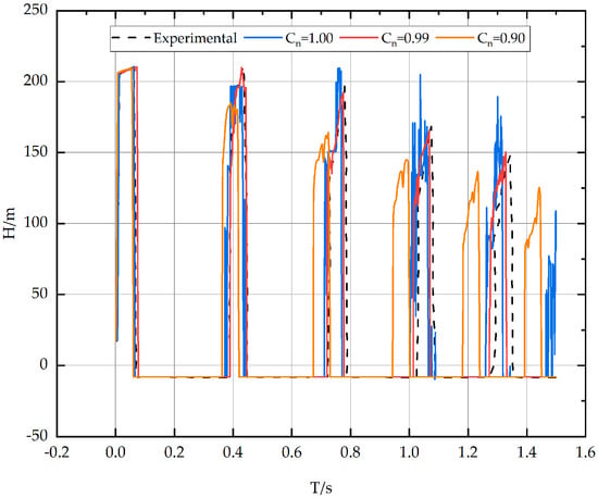
Figure 2.
Comparison of Cn prediction results of three groups.
When Cn is close to 1 (e.g., 0.99), the model prediction accuracy is high; when Cn is exactly 1, the prediction results will have violent numerical oscillations, which will affect the prediction effect; and when Cn is low (e.g., 0.90), the numerical dissipation generated in the process of simplifying the differential equation into a difference equation is too large, which has a more noticeable effect on the time and intensity of the occurrence of the bridging water strike [15].
Balancing numerical stability and computational accuracy is often a dilemma in numerical computations. This paper uses the Muskingum method [16] to address this contradiction and improve the traditional discrete vaporous cavity model (DVCM). As a widely adopted river flow evolution algorithm, the Muskingum method determines parameter factors through trial calculations. It utilizes the error of the finite difference numerical solution of the kinematic wave equation to compensate for the physical diffusion term of the diffusive wave. This ensures that the numerical solution is the exact solution of the diffusive wave equation. Inspired by this method, this paper analyzes the simulation process’s relationship between numerical and physical dissipation. It innovatively proposes adjusting the physical dissipation in the water hammer program to compensate for numerical dissipation in the calculations. This approach effectively improves the predictive accuracy of the DVCM and provides a new idea for enhancing computational accuracy in numerical simulations in other fields.
2. Research Methodology
2.1. MOC Algorithm Overview
For the small fluid element in the pipeline shown in Figure 3, a force analysis is conducted to derive the motion and continuity differential equations. These equations are then simplified to form a pair of quasilinear hyperbolic differential equations, denoted as L1 and L2:
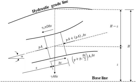
Figure 3.
Force Analysis on a Small Fluid Element in a Pipeline.
By introducing the characteristic factor x and simplifying L1 and L2, the characteristic line equations can be obtained as follows:
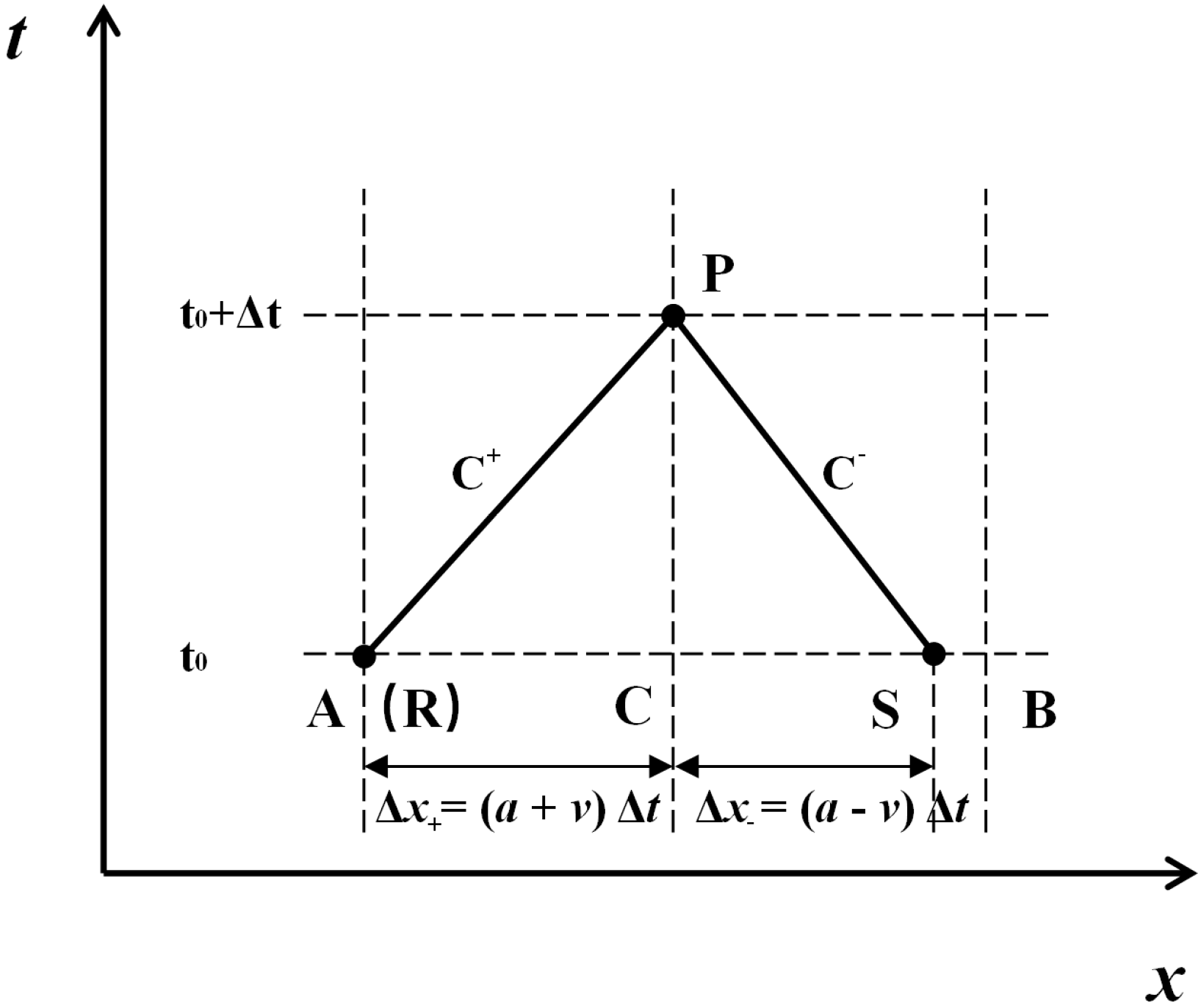
Through the above transformation, the original two partial differential equations are converted into two ordinary differential equations using the method of characteristics. Each is accompanied by a constraint condition and restricted to the specific paths described by the corresponding characteristic line equations, as shown in Figure 4.
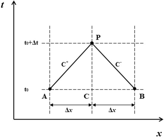
Figure 4.
Characteristics in the x-t plane.
Assuming that the dependent variables h and q are known at points A and B on a given characteristic line, integrating along the two characteristic lines allows the solution of the characteristic line equations (Equation (3)):
Letting , , the above equation can be rewritten as
Then, using the equations above, the values of HP and QP at point P can be determined:
2.2. DVCM Algorithm Overview
DVCM assumes [17,18] that there is no gas in the initial stability of the pipeline; in the process of hydraulic transition, when the pressure at a node of the pipeline is lower than the saturation vapor pressure of the liquid, it is considered that the vapor generated by the vaporization of the liquid is concentrated in the cross-section of the calculation node, the head in the vapor cavity remains unchanged, and the pressure at the boundary is equal to the pressure inside the vapor cavity; when the vapor cavity collapses, the head and flow at the node can still be solved using the method of characteristic lines.
The simulation process of water–column separation and its reconnection boundary conditions can be carried out through the following specific computational steps.
- Determine whether water column separation occurs.
The absolute pressure at the cross-section of node i can be expressed as
Among them, the condition for liquid column separation to occur is .
- 2.
- Calculate liquid column separation.
When node i is in a state of liquid column separation, the transient parameters can be calculated using the following formulas:
Furthermore, the flow rate of the cavity formed by liquid column separation can be expressed by the rate of change in the cavity’s volume, as shown in Equation (8):
Furthermore, the volume formula for the cavity formed by liquid column separation can be simplified to Equation (9):
- 3.
- Increase the pressure after reconnection.
If during the calculation process, it is considered that the water column reconnects at that instant, and the transient parameters can be calculated using the following formulas:
When calculating node i, first determine the gas volume at the previous time step. If gas is present, the node is considered a liquid column separation boundary, and the node head, inlet flow rate, outlet flow rate, and gas cavity volume at time step j can be directly calculated using Equations (7)–(9). If no gas is present, further assess whether the node head Hpi is below the cavitation pressure. If it is below the cavitation pressure, the node is transformed into a boundary point with the pressure headset as the airhead. Subsequently, the inlet flow rate, outlet flow rate, and gas cavity volume at time step j are calculated using the continuity and characteristic line equations. If the node head is above the cavitation pressure, liquid column separation and reconnection are deemed to occur, and Equation (10) is employed for the calculation.
In all the above calculations, the wave velocity of water strikes in the piping system is unaffected by the gas volume change. When the liquid column separation phenomenon occurs, the wave velocity of the water column is considered to remain constant between the inner node and the outer node because all the generated gas is concentrated at the inner node. The specific calculation steps are shown in Figure 5.
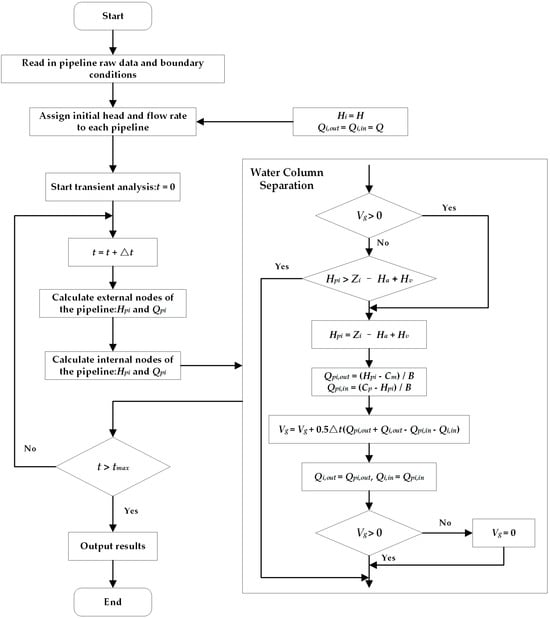
Figure 5.
Flowchart of DVCM calculation.
2.3. Numerical Dissipation Compensation Methods
In engineering, only physical dissipation, such as along-travel head loss and local head loss, exists in the pipeline where liquid column separation occurs. In the hydraulic transition process, the physical dissipation is mainly reflected in the along-travel head loss [19,20]; according to the formula, the along-travel head loss is positively correlated with the resistance coefficient f. When using DVCM to simulate liquid column separation, the program will generate additional numerical dissipation, which leads to distortion of the prediction results. To solve the above problems, in this paper, the numerical dissipation is equivalently converted to the physical dissipation, and the total dissipation calculated by the program is the same as the actual total dissipation by adjusting the physical dissipation (i.e., the drag coefficient f) downward to improve the accuracy of the model calculation.
2.3.1. Evaluation of Error Model (EAM)
This paper introduces two metrics to assess the degree of influence of different parameters on the prediction results, namely the numerical dissipation error metric Xn and the physical dissipation error metric Xm. The peak head lift and the column separation time of [21] are chosen as the constituent factors in the metrics.
To calculate the numerical dissipation error index Xn, for example, taking into account that when the value of Cn is 1, the prediction results are prone to numerical oscillation phenomenon, Cn tends to 1, the differential equation is simplified to the difference equation generated by the truncation error caused by the numerical dissipation of close to negligible, this paper takes the prediction results when Cn is 0.99 as a benchmark and calculates the relative error of model prediction with different Cn, as shown in Equation (11):
The physical error index Xm is calculated in the same way as above. In this paper, the relative error of the model at different f is calculated as shown in Equation (12). After taking the drag coefficient f of 0.0245 (experimental value) as the benchmark:
where is the head error weight, is the time error weight, n is the number of times liquid column separation occurs at the node, H is the nodal head, T is the nodal liquid column separation time, and x is the value of Cn or f corresponding control group.
2.3.2. Assessment of the Level of Numerical Dissipation
Taking a single simple pipe as an example, when Cn is 1, there will be apparent numerical oscillations, and when it is 0.99, the numerical dissipation is minimal and no numerical oscillations occur. Five different numerical errors Xn are obtained when the Cn values are 0.99, 0.95, 0.9, 0.85, and 0.8, respectively. The Xn value decreases gradually as the Cn decreases, and the numerical dissipation increases. The calculation results will be plotted on the graph, which can be Xn and Coulomb number Cn of the change rule. Take a simple pipe as an example; this paper simulates five groups of different f values corresponding to the calculation of working conditions. As the resistance coefficient f decreases, the physical dissipation gradually decreases, Xm gradually increases, and when f is 0, the predicted value of the overestimation level reaches the peak and Xm reaches the maximum value. The results of the calculations are plotted on a graph to obtain the pattern of change of Xm concerning the drag coefficient f (refer to the following example for verification).
2.3.3. Parameter Optimization
When the sum of the numerical and physical error factors is close to zero (Xn + Xm ≈ 0), the numerical dissipation is compensated by reducing the physical dissipation, which improves the accuracy of the model calculations and brings the results closer to the real solution.
This strategy can be extended to series and bifurcated complex piping systems. Before the numerical simulation, trial calculations are first carried out for each pipeline separately to obtain its numerical dissipation error factor Xn. By adjusting the physical dissipation error factor Xm of each pipeline network, the additional numerical dissipation is compensated separately, which improves the accuracy of the model calculations and ensures numerical stability.
3. Instance Validation
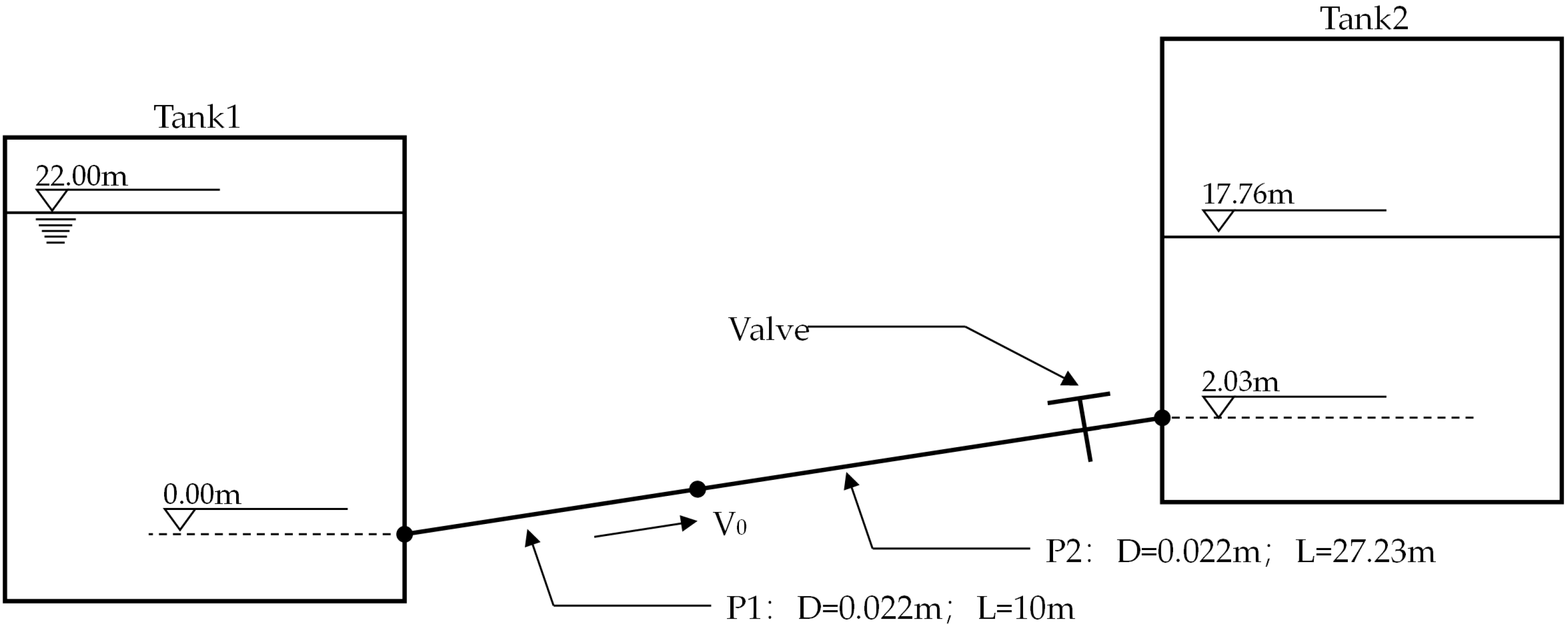
This paper validates the liquid–column separation experiments carried out with the experimental setup built by Bergant and Simpson from the University of Adelaide, Australia. The model sketch is shown in Figure 6.
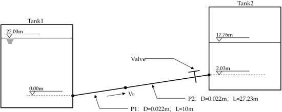
Figure 6.
Diagram of the experimental model.
In the experiment, water flowed from water tank 1 through the upstream pipeline to water tank 2. The upstream water tank’s normal storage level was 22 m, and the downstream water tank’s storage level was 17.76 m. The water tank diversion pipeline’s inlet elevation was 0 m and its outlet elevation was 2.03 m. The experiments measured the steady-state pipeline flow velocity V0 as 1.4 m/s, corresponding to a pipeline resistance coefficient f of 0.0245. The pipeline computational model parameters are as follows (Table 1).

Table 1.
Parameters of the pipeline calculation model.
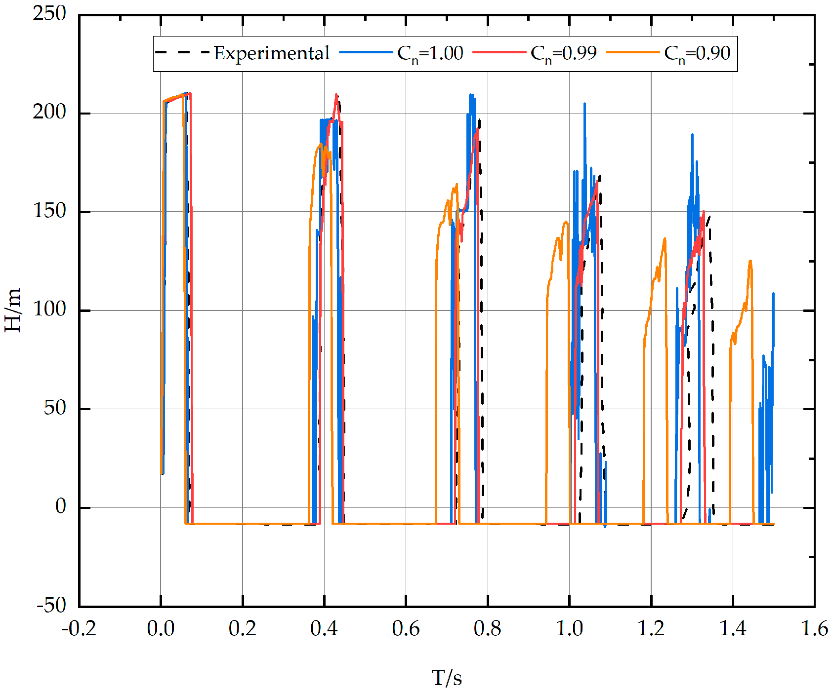
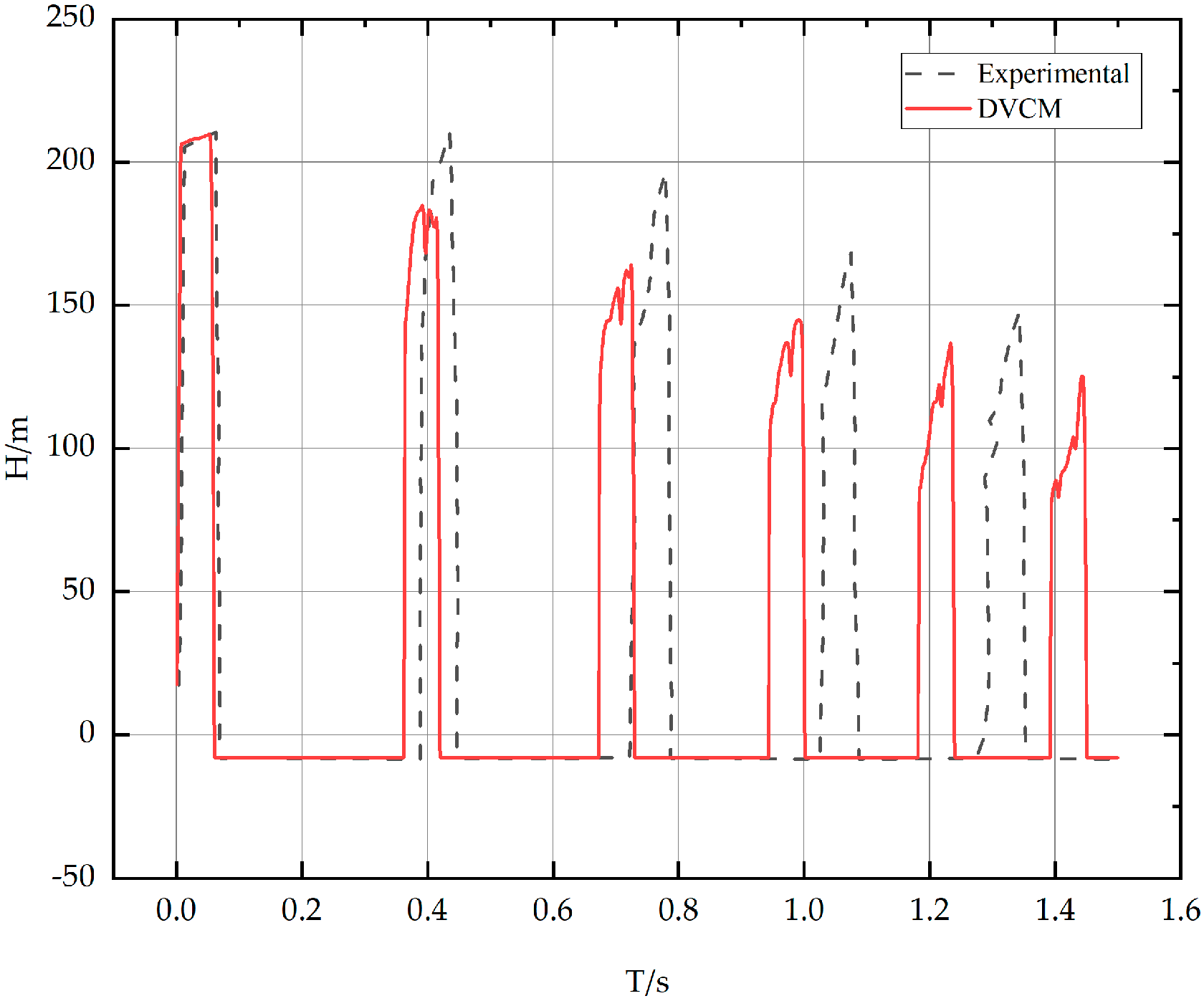
The upstream and downstream Coulomb numbers Cns of the valves were 0.99 and 0.93, respectively, at the time of calculation. During the operation, the downstream valve was suddenly closed, and the closure time was 0.006 s. The measured results at the valves and the predicted results of the DVCM are shown in Figure 7 below. The calculation results show that the model predicts that the peak head at the node at the valve is low compared with the experimental value, and the phase front shift is too significant. It indicates that the numerical dissipation of the program in the calculation is relatively large, causing error accumulation which affects the DVCM prediction results.
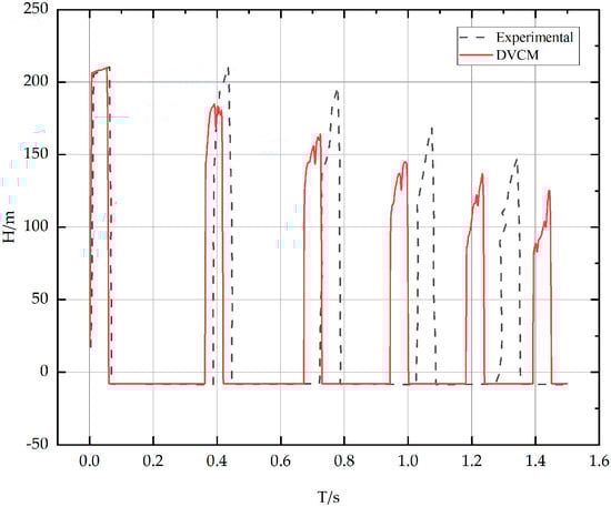
Figure 7.
Distribution of head at valve with time.
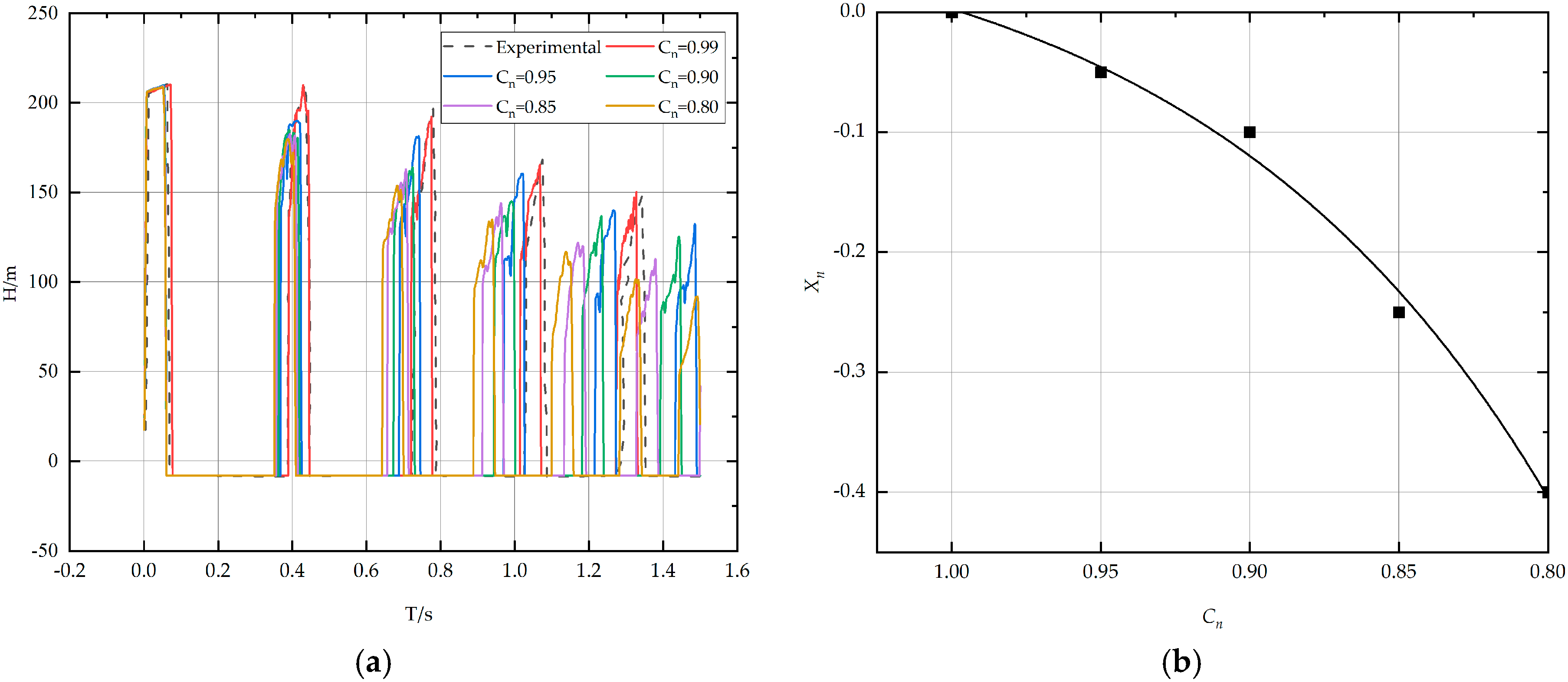
- Analysis of the effect of Cns
The Cn = 0.99 corresponds to P1 in the calculation process. It can be assumed that the numerical dissipation of P1 can be neglected during the transient flow simulation and only the numerical dissipation of P2 needs to be evaluated. Keeping the resistance coefficient consistent with the experimental value, five different Cn combinations are taken for P2 from large to small for trial calculation. The calculation to obtain the node pressure fluctuation at the valve is shown in Figure 8a, and Equation (11) is used to calculate the numerical error factor corresponding to different Cns, respectively. The trend change in Figure 8b is shown in Figure.
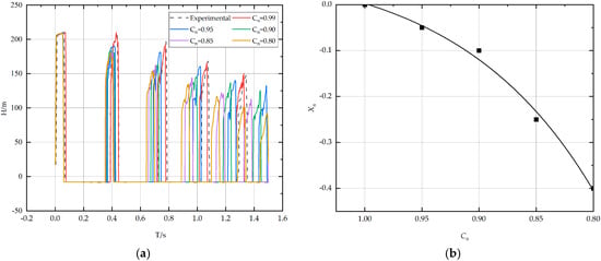
Figure 8.
(a) Distribution of head at valve with time at different Cns; (b) trend of Xn with different Cns.
According to the analysis of the above figure, when the Coulomb number Cn corresponding to P2 is not equal to 1, the internal interpolation will cause additional numerical dissipation, resulting in low head boost and column separation time in the simulation results as well as low peak predicted head and phase forward shift. As the Cn decreases, the resulting numerical dissipation gradually increases, leading to a faster rate of energy decay within the system and a gradual increase in the errors in the head rise and column separation times.
- 2.
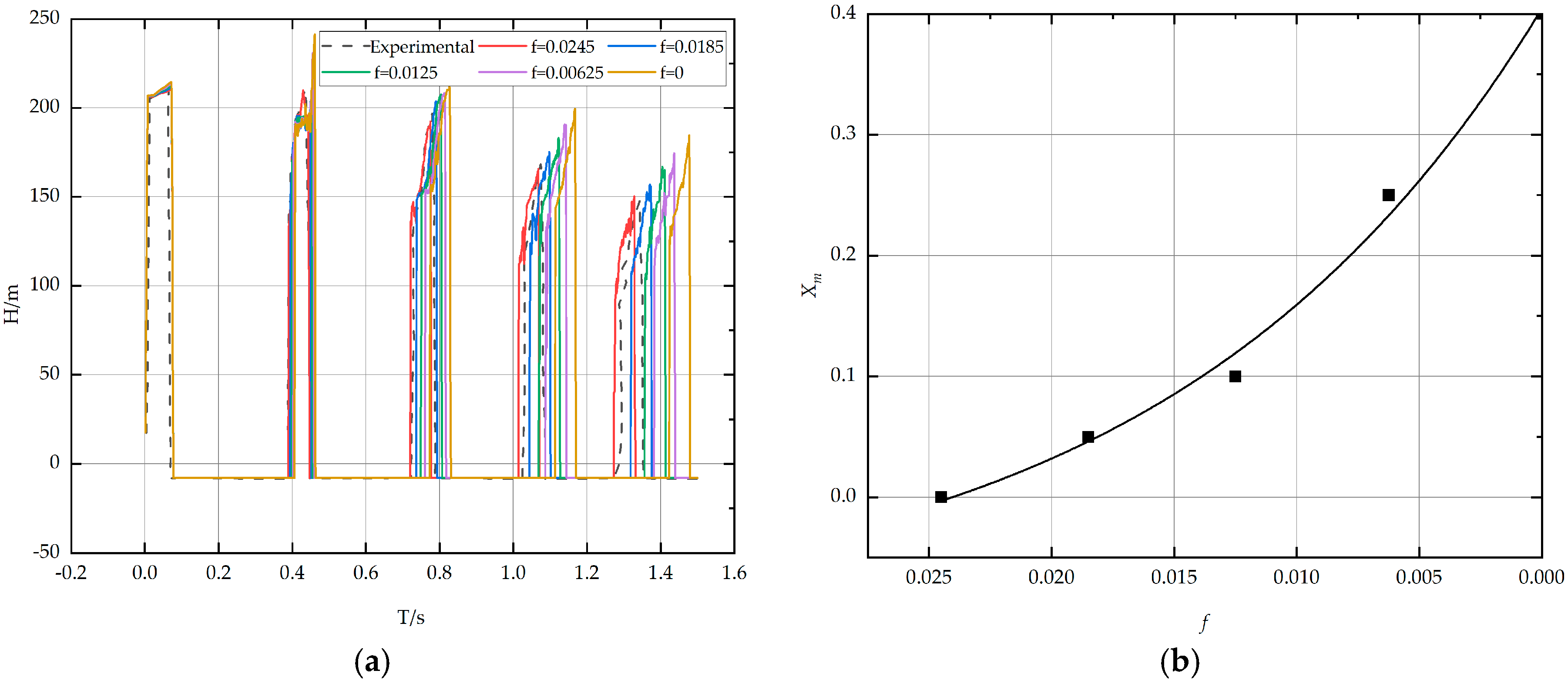
- Impact analysis of the drag coefficient f
To assess the influence of physical dissipation in P2 on the model’s prediction accuracy, this paper sets the calculation results, when the Coulomb number corresponding to P1 and P2 is 0.99, as the baseline and adopts different P2 to calculate the interference of numerical dissipation on the simulation results. It is calculated to obtain the node pressure fluctuation at the valve Figure 9a, as shown in Figure 9. Then, Equation (12) calculates the physical error factor corresponding to different fs, respectively, and plots the trend change of Figure 9b, as shown in Figure 9.
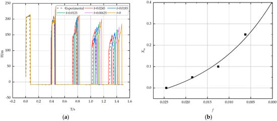
Figure 9.
(a) Distribution of head at valve with time for different fs; (b) trend of Xm at different f.
Through the analysis of Figure 9a,b, it is found that when the resistance coefficient f set in the program is smaller than the actual value, the physical dissipation is lower than the actual value, which causes the head boosting and liquid–column separation time in the simulation to lag behind the experimental value. As the resistance coefficient f corresponding to the pipeline set in the program gradually decreases, the resulting physical dissipation also gradually decreases, the internal energy decay rate of the system slows down, and the overestimation level of the simulated head boost and liquid column separation time gradually increase.
- 3.
- Analysis of the relationship between Cn and f parameters
Based on the compensation strategy of numerical dissipation and physical dissipation, when Xn + Xm ≈ 0, the best accuracy prediction result will be obtained. Combining the error trend data in Figure 8b and Figure 9b, the correlation between Cn and f can be plotted as seen in Figure 10.
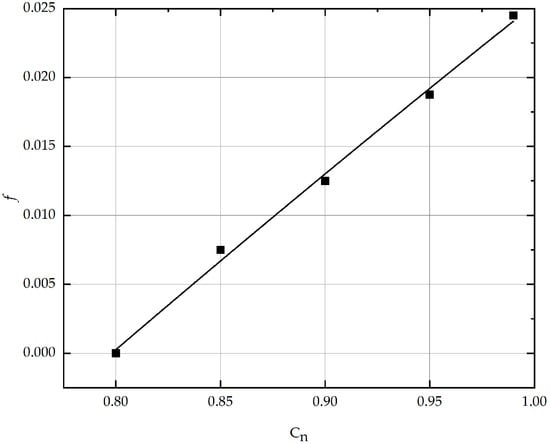
Figure 10.
Optimal correspondence between Cn and f.
- 4.
- Numerical dissipation compensation
When Cn2 takes the value of 0.93, there will be a significant numerical dissipation phenomenon. To effectively reduce the adverse effect of numerical dissipation on the model prediction accuracy, this study uses the parameter correspondence shown in Figure 10 to take f2 as 0.013. Through this artificial adjustment, the additional loss introduced by numerical dissipation is compensated by reducing physical dissipation so that the total dissipation level in the numerical computation is close to the same as the actual physical total dissipation level, and the prediction accuracy of the DVCM can be significantly improved. The results are shown in Figure 11a,b below.
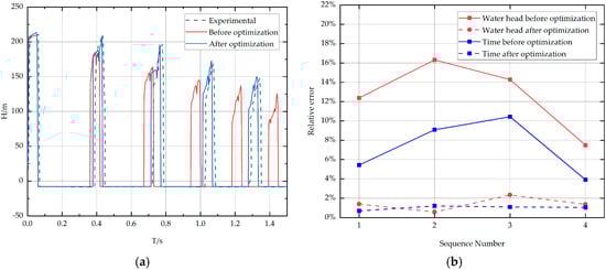
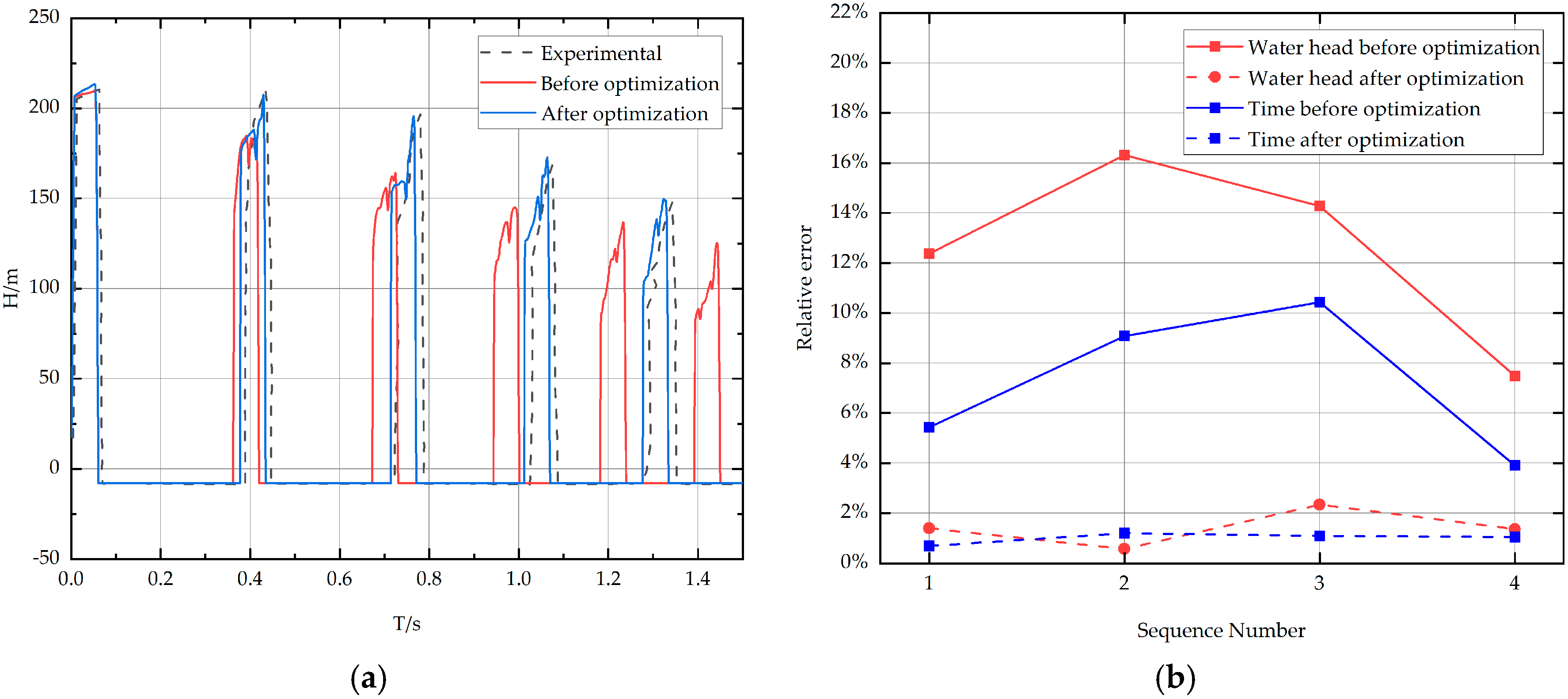
Figure 11.
(a) Comparison of head optimization at the valve; (b) comparison of relative errors of head and time.
The change in head at the valve before and after optimization is compared in Figure 11a,b. Before the parameter optimization, the numerical dissipation generated by the program calculation is more significant, resulting in higher energy dissipation within the system than in the actual situation. The peak head values of the four bridging boosts in the predicted results are lower than the actual head. The first two predicted heads have more significant relative errors, 12.38% and 16.32%, respectively. The four-times liquid column separation time is lower than the actual time, and the relative error of the predicted values gradually increases, resulting in the gradual forward shift in the expected phase. After improvement, the accuracy of the peak head prediction of the four bridging boosts in the calculation results is significantly improved, and the relative error of the maximum bridging water strike is controlled within 2.34%. The separation time of the four liquid columns is similar to the actual time, and the relative error of the predicted value is stabilized within 1.19%. The numerical dissipation introduced to ensure the computational stability is significantly compensated, the change in water head tends to be consistent with the actual situation, and the model’s prediction accuracy is improved considerably.
4. Conclusions and Future Work
4.1. Conclusions
In this paper, the method of mutual compensation between numerical and physical dissipation is proposed to improve the simulation of the liquid–column separation process of DVCM in complex pipelines, and good results are achieved. The following experiences are obtained in the research process for the reference of related researchers:
- When the characteristic line calculation is used when the Coulomb number Cn deviates from 1; the prediction results of the model will significantly deviate, resulting in lower predicted values of the nodal head rise and liquid–column separation time compared with the actual values. The Courant number in pipeline calculations is an important parameter to ensure the accuracy and reliability of numerical simulations. The model’s energy dissipation significantly impacts the calculation accuracy of the bridging water hammer.
- This paper observes that the total dissipation during numerical calculations can be finely tuned by adjusting the resistance coefficient f of the pipeline without affecting the numerical stability.
- Drawing on Muskingum’s method, reversing the operation to adjust the physical dissipation to compensate for the numerical dissipation can significantly improve the prediction accuracy of the numerical computation of the bridging water strikes in this paper. When the numerical dissipation is balanced with the physical dissipation, the relative errors of the peak head and liquid–column separation time at the DVCM prediction nodes are reduced to under 6%. The strategy of mutual compensation between physical and numerical dissipation not only improves the prediction accuracy of DVCM but also provides new ideas for other numerical simulations to improve computational accuracy and stability.
4.2. Future Work
Building on the research presented in this paper, future directions can be explored to further enhance the accuracy and practicality of simulating liquid–column separation phenomena:
- Application and optimization in real-world operational environments
Our ultimate goal is to collaborate closely with municipal water supply departments and industry partners to apply the methods proposed in this study to real-world operational settings and test their applicability in actual pipeline systems. We believe such collaboration will provide valuable insights to help us refine and optimize our models to address larger-scale and more complex pipeline networks. This interdisciplinary cooperation will not only advance theoretical research but also strongly support the safe operation and optimal design of municipal water supply systems.
- 2.
- Consideration and response to unsteady friction in future simulations
In future simulation studies, we will consider steady-state friction and further investigate the impact of unsteady friction on liquid–column separation phenomena, as well as explore corresponding countermeasures. Unsteady friction can significantly influence pressure fluctuations and the dynamic behavior of liquid—column separation during transient flow. By incorporating unsteady friction models, we can more accurately simulate the complex flow conditions in real pipeline systems. This provides a more reliable theoretical basis for water hammer protection and pipeline system design.
Author Contributions
Conceptualization, W.C. (Wenhao Chen); data curation, Z.L.; investigation, L.P. and Y.J.; methodology, W.C. (Wenhao Chen); writing—original draft, W.C. (Wenhao Chen); and writing—review and editing, W.C. (Weiping Chen) and J.J. All authors have read and agreed to the published version of the manuscript.
Funding
This research was funded by a Provincial/Ministerial-level Fund in China (Grant No.: 2022-K-161).
Data Availability Statement
The data presented in this study are available on request from the corresponding author.
Conflicts of Interest
Author Zhihong Long was employed by the company Guangzhou Water Supply Co., Ltd. Author Liyun Peng and Yonghong Jiang were employed by the company Hangzhou Leadmap Information Technology Co., Ltd. All authors declare that the research was conducted in the absence of any commercial or financial relationships that could be construed as a potential conflict of interest.
Abbreviations and Glossary
The following abbreviations and glossary are used in this manuscript:
| DVCM | Discrete vaporous cavity model |
| DGCM | Discrete gaseous cavity model |
| TFM | Two-fluid mathematical model |
| CFL | Courant–Friedrich–Lewy |
| EAM | Evaluation of error model |
| Courant number | |
| Spatial distance | |
| Spatial interpolation on the right side | |
| Spatial interpolation on the left side | |
| Initial calculation time | |
| Minimum calculation time interval | |
| Node water head | |
| Time | |
| Steam volume at node i at time j in the pipeline | |
| Head at node i at the next time step in the pipeline | |
| Flow rate at node i at the next time step in the pipeline | |
| Elevation at node i in the pipeline | |
| Atmospheric pressure head | |
| Vapor pressure head of water | |
| The flow rate into node i at the previous time step | |
| The flow rate into node i at this moment | |
| Flow rate out of node i at the previous time step | |
| Flow rate out of node i at this moment | |
| Characteristic parameters of the method of characteristics | |
| Characteristic parameters of the method of characteristics | |
| Characteristic parameters of the method of characteristics | |
| Maximum calculation time | |
| Friction coefficient | |
| Numerical dissipation error index | |
| Physical dissipation error index | |
| Weight of peak water head | |
| Weight of liquid–column separation duration | |
| The peak water head at node i in the pipeline when the courant number is equal to x | |
| The peak water head at node i in the pipeline when the friction coefficient is equal to x | |
| The duration of liquid–column separation at node i in the pipeline when the courant number is equal to x | |
| The duration of liquid–column separation at node i in the pipeline when the friction coefficient is equal to x | |
| Pipe diameter | |
| Pipeline length | |
| Wave speed | |
| Time interval | |
| Spatial interval |
References
- Zhou, L.; Wang, N.; Zhao, Y. Godunov model for water column separation and water hammer considering dynamic friction. J. Harbin Inst. Technol. 2023, 55, 138–144. [Google Scholar]
- Adamkowski, A.; Lewandowski, M. Investigation of hydraulic transients in a pipeline with column separation. J. Hydraul. Eng. 2012, 138, 935–944. [Google Scholar] [CrossRef]
- Fu, Y.; Xie, C.; Jiang, J. Calculation and study on the secondary pressure surge phenomenon of water hammer under liquid column separation. J. China Three Gorges Univ. (Nat. Sci. Ed.) 2022, 44, 88–94. [Google Scholar]
- Liu, Z.X.; Liu, G.L. Pump Station Water Hammer and Its Protection; Water Resources and Electric Power Press: Beijing, China, 1988; pp. 107–108. [Google Scholar]
- Zhang, Q.; Yan, Y.; Huang, B. Experimental study on transient flow characteristics of leakage in air-containing water conveyance pipelines. J. Hydrodyn. Ser. A 2022, 37, 678–683. [Google Scholar]
- Streeter, V.L. Water hammer analysis. J. Hydraul. Div. 1969, 95, 1959–1972. [Google Scholar] [CrossRef]
- Wiggert, D.C.; Sundquist, M.J. The effect of gaseous cavitation on fluid transients. J. Fluids Eng. 1979, 101, 79–86. [Google Scholar] [CrossRef]
- Wylie, E.B. Simulation of vaporous and gaseous cavitation. J. Fluids Eng. 1984, 106, 307–311. [Google Scholar] [CrossRef]
- Fu, Y.; Jiang, J.; Li, Y.; Ying, R. A Two-Fluid Model-Based Calculation Method for Gas-Liquid Two-Phase Water Hammer. J. Huazhong Univ. Sci. Technol. (Nat. Sci. Ed.) 2018, 46, 126–132. [Google Scholar]
- Hu, L.R. Verification and Application of a Water Hammer Model Based on Discrete Steam/Gas Cavitation Theory. Master’s Thesis, Lanzhou University of Technology, Lanzhou, China, 2023. [Google Scholar]
- Zhou, L.; Lu, Y. SWMM Simulation Capability for Transient Flow in Drainage Pipe. China Water Wastewater 2022, 38, 108–115. [Google Scholar]
- Cai, Y.; Sheng, J. Research on the fast and high-precision characteristic line method analysis of hydraulic pipelines. J. Zhejiang Univ. 1986, 3, 35–46. [Google Scholar]
- Wang, B.Q. Numerical Calculation of Water Hammer Due to Flow Reconnection Based on the Lattice Boltzmann Method. Master’s Thesis, Harbin Institute of Technology, Harbin, China, 2017. [Google Scholar]
- Bergant, A.; Simpson, A.R. Estimating unsteady friction in transient cavitating pipe flow. In Proceedings of the 2nd International Conference on Water Pipeline Systems, Edinburgh, UK, 24–26 May 1994. [Google Scholar]
- Niu, L.; Jing, H.; Li, P. Numerical simulation of water hammer considering unsteady friction and cavitation. J. Appl. Mech. 2023. Available online: https://kns.cnki.net/nzkhtml/xmlRead/trialRead.html?dbCode=CAPJ&tableName=CAPJTOTAL&fileName=YYLX20230717002&fileSourceType=1&invoice=d%2bwJ0BWJmTkiULjORYDHPU0khEjm7WoGUZTAGfIO2Agi59NZGH8wZUQgeMQLjF9O46XMRCaqd8GOIE7CCJQ8ftEKcLzzDkBzSBmFZUF1Oq96erTvgXPyfV8VlhxEGJZyUeo6ybGNMROqKwKqixUqr2ycHRUbZ40sDVZXeRgBcO4%3d&appId=KNS_BASIC_PSMC (accessed on 17 February 2025).
- Yang, F.; Jiang, E.; Wang, Y. Sediment transport calculation of multi-sand rivers based on the Muskingum method. People’s Yellow River 2023, 45, 39–42. [Google Scholar]
- Wen, D.D. Theoretical Study and Numerical Simulation of Water Hammer Due to Flow Reconnection and Its Protection. Master’s Thesis, Southwest Petroleum University, Chengdu, China, 2015. [Google Scholar]
- Santoro, V.C.; Crimì, A.; Pezzing, A. Developments and limits of discrete vapor cavity models of transient cavitating pipe flow: 1D and 2D flow numerical analysis. J. Hydraul. Eng. 2018, 144, 04018047. [Google Scholar] [CrossRef]
- Jamil, R. Frictional head loss relation between Hazen-Williams and Darcy-Weisbach equations for various water supply pipe materials. Int. J. Water 2019, 13, 333–347. [Google Scholar] [CrossRef]
- Chen, Y.; Du, Y.; Geng, A. Discussion on the Calculation Method of Head Loss Along the Pipeline in Water Supply and Drainage. J. Water Wastewater 2009, 45, 109–111. [Google Scholar]
- Li, Z.; Fan, C.; Shen, H. A New Cavity Model for Water Hammer with Liquid Column Separation. J. Hydraul. Eng. 2024, 44, 37–41+53. [Google Scholar]


Disclaimer/Publisher’s Note: The statements, opinions and data contained in all publications are solely those of the individual author(s) and contributor(s) and not of MDPI and/or the editor(s). MDPI and/or the editor(s) disclaim responsibility for any injury to people or property resulting from any ideas, methods, instructions or products referred to in the content. |
© 2025 by the authors. Licensee MDPI, Basel, Switzerland. This article is an open access article distributed under the terms and conditions of the Creative Commons Attribution (CC BY) license (https://creativecommons.org/licenses/by/4.0/).