Article

Evaluation of Various Land Use Metrics for Enhancing Stream Water Quality Predictions

1
Civil Engineering Department, King Saud University, P.O. Box 800, Riyadh 11421, Saudi Arabia
2
Civil and Environmental Engineering, Texas A&M University, College Station, TX 77840, USA
3
Glenn Department of Civil Engineering, Clemson University, Clemson, SC 29634, USA
*
Author to whom correspondence should be addressed.
Water 2025, 17(6), 849; https://doi.org/10.3390/w17060849
Submission received: 13 February 2025 / Revised: 12 March 2025 / Accepted: 13 March 2025 / Published: 16 March 2025

Abstract

:
Water quality in streams is primarily affected by various land use practices. This study analyzes water quality data collected from the outlets of 113 watersheds across three South Atlantic states in the USA. The objective is to evaluate the relationship between different land use metrics and long-term stream water quality, specifically investigating whether incorporating the spatial proximity of various land uses to the stream and outlet can enhance predictions of stream water quality. To achieve this, four distinct metrics were utilized to assess their influence on stream water quality. The first metric, known as the Lumped method, assigns equal weight to all land uses. The second, the Inverse Distance Weights stream (IDWs), gives greater weight to land uses located closer to the stream. The third metric, the Inverse Distance Weights Outlet (IDWO), weights land uses according to their proximity to the watershed outlet. The final metric focuses on hydrologically sensitive areas (HSAs), which are areas within watersheds that generate the majority of runoff. The results indicated that the Lumped metric emphasizes the significance of forested lands, whereas the HSAs, IDWs, and IDWO metrics highlight the importance of the spatial distribution of agricultural and industrial lands within the watershed. These findings support the hypothesis that considering hotspot areas and their relative positions within the watershed can improve predictions of water quality. Overall, the incorporation of HSAs, IDWs, and IDWO metrics shows that not only is the extent of land use change within a watershed critical, but also the proximity of these land uses to a stream or outlet plays a significant role.

1. Introduction

Urban and agricultural land use significantly impacts the hydrological, biogeochemical, and biological processes within aquatic ecosystems, often leading to water quality degradation [1,2,3,4]. Moreover, the effects of anthropogenic land use changes have emerged as a global concern, contributing to the degradation of aquatic ecosystems [5,6,7]. Consequently, extensive research in recent decades has concentrated on the effects of these land use changes on stream water quality [8,9,10].
Previous research has mainly examined the relationships between land uses within a watershed and the quality of downstream water [5,6,7,8,9]. However, the spatial metrics and variations in water quality degradation are influenced by factors such as topography, soil composition, and biogeochemical characteristics [10,11]. Therefore, further research is essential to effectively identify the processes that connect land use alterations to water quality deterioration.
The impacts of land use changes on water quality are generally recognized as spatially dependent [7,12,13]. Previous research has mainly focused on the Lumped method to represent landscape alterations and evaluate their effects on water quality [10]. To illustrate, the proportion of urban land within the watershed has often been estimated to evaluate the extent of urban influences on stream water quality, commonly without considering the spatial distribution of these land uses [2]. Such non-spatial (or Lumped) methods may inadequately capture the impact of urban land on streams, as they generally operate under the assumption that each land use segment exerts an equal influence on stream water quality. This assumption can result in misleading conclusions regarding the connection between land use changes and stream water quality [14,15,16].
Three methods have been proposed to address the limitations associated with simplistic non-spatial representations of land use. The first method uses an inverse distance-weighted (IDW) method to evaluate the relationship between land use and stream water quality (Peterson et al., 2011 [16]). This method assigns more weight to land uses closer to the river or watershed outlet to assess the impacts on water quality [14,16]. The second method focuses on land uses in riparian zones instead of considering the entire watershed to evaluate their effects on water quality [17,18,19]. For instance, densely vegetated riparian zones, such as forests, are expected to reduce nutrient and sediment loads and influence the energy balance within streams [20,21]. Although these findings emphasize the importance of land use in riparian areas, how large the width of riparian zones necessary for effective management remains inadequately determined [22]. Recent studies have investigated the connection between land use and water quality, using the concept of hydrologically sensitive areas (HSAs) [10,23]. HSAs are defined as areas within the watershed that produce the majority of runoff during heavy rainfall events. Previous studies have shown that examining land use in HSAs can provide a more effective means of assessing downstream water quality than evaluating the entire watershed [10,23,24]. Overall, it has been shown that these saturated areas within a watershed are significant contributors to the generation and transport of pollutants to streams [10,23,25].
While numerous previous studies have utilized the HSAs (hydrologically sensitive areas) concept to identify best management practices (BMPs) for mitigating nonpoint source pollution, the focus has predominantly been on agricultural and urban lands at small watershed scales. Moreover, much of the existing research operates under the assumption that BMPs applied in HSAs enhance water quality more effectively. However, there remain gaps in the literature regarding direct quantitative comparisons across various watershed metrics. Specifically, few studies have assessed how land use in HSAs compares with other spatial metrics, such as Lumped and Inverse Distance Weighting (IDW), which examine the influence of land uses closer to the stream and outlet on water quality within a broader watershed context.
This study aims to link this gap by evaluating the impact of land use using Lumped, IDW (distance to stream and outlet), and HSAs metrics on stream water quality. The hypothesis is that, despite their limited extent within a watershed, land uses evaluated at HSAs and using IDW metrics have a more pronounced effect on water quality compared to those in other watershed areas. Validating this hypothesis is a crucial step toward developing more effective watershed management strategies. If confirmed, this could enable watershed managers to prioritize BMP implementation in HSAs and IDW metrics, ultimately resulting in a more cost-effective approach to improving water quality.

2. Materials and Methods

2.1. Study Area

The study area comprises 113 watersheds (Figure 1) across three states: North Carolina, South Carolina, and Georgia. The study area is distributed among three physiographic regions (the coastal plain, the Blue Ridge, and the Piedmont). Initially, 320 watersheds were delineated using a 10 m Digital Elevation Model (DEM). In this study, 113 watersheds were chosen based on three criteria (Alnahit et al., 2020 [11]): (1) nested watersheds were excluded to prevent water transfer from external watersheds; (2) watersheds where reservoirs occupied more than 25% of the total area were excluded; and (3) watersheds with water quality monitoring stations located less than 50 km downstream from a reservoir were removed. The evaluated watersheds range in size from 24 km2 to 2062 km2. Land use within these watersheds varies widely, encompassing natural wetlands, grasslands, forests, agricultural areas, and urban developments (Table 1). The agricultural lands include both croplands and pastures, with the primary crops being corn, soybeans, and cotton.

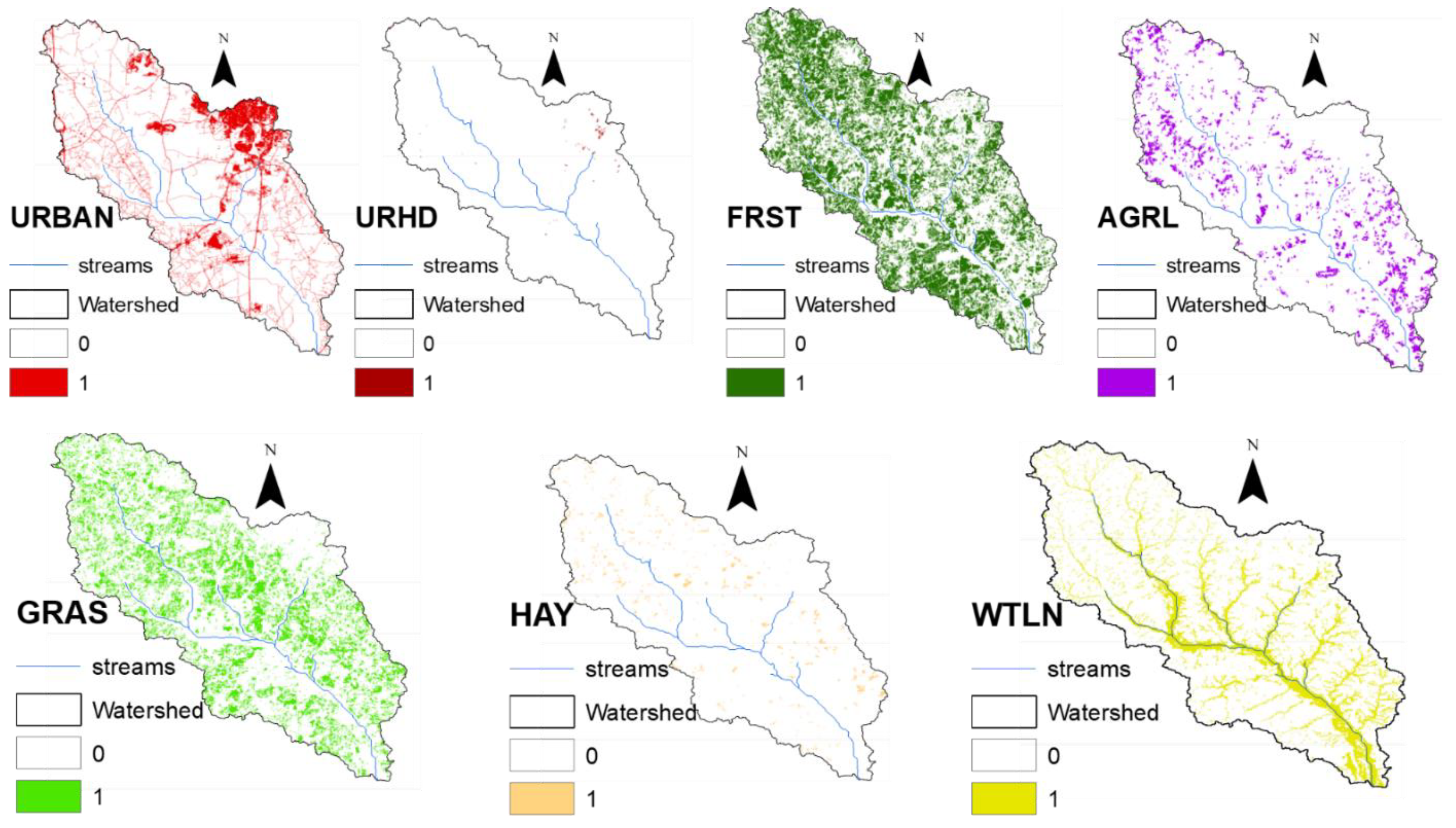
2.2. Land Use and Water Quality Monitoring Data

The land use data used in this study are listed in Table 1. These variables were downloaded from the National Land Cover Dataset (NLCD) [26]. For each watershed, the areas corresponding to various land use categories (shown in Table 1) were obtained from the 2011 land use/cover data. The land use data from 2011 was chosen to serve as an average representation of land use from 2000 to 2020 [11,27]. High-density urban land is characterized by densely populated areas containing either high-density single units or more than 100 units per hectare. Medium-density urban land comprises residential units ranging from more than 30 to less than 100 per hectare, while low-density urban land includes fewer than 30 units per hectare [26]. The land use matrices represent the percentage of each land use type within each watershed, and the high-density, medium-density, and low-density urban lands were aggregated into a single category (URBAN) to better assess the impact of urbanization on stream water quality.
Monthly water quality data covering the period from 2000 to 2020, including total nitrogen (TN), total phosphorus (TP), and turbidity (TUR) measurements for each outlet, were evaluated in this study. Total nitrogen (TN) encompasses the overall nitrogen present in a sample, including various forms such as nitrate, nitrite, and ammonia. Total phosphorus (TP) represents the total phosphorus in a sample, including both dissolved and particulate forms. Turbidity (TUR) indicates the cloudiness or haziness of a fluid caused by suspended particles, and it serves as a key indicator of water quality.
TN, TP, and TUR at the outlet of each watershed were downloaded from publicly available water monitoring databases using the “dataRetrieval” package in R version 4.0.0 [28]. This package provides access to water quality data from the U.S. Geological Survey (USGS) and the Environmental Protection Agency (EPA). After that, the retrieved datasets were preprocessed to ensure consistency across the time period. Water quality measurements were reported as concentrations (mg/L) for TN and TP, and as nephelometric turbidity units (NTUs) for TUR. Before averaging the water quality data at each watershed outlet, a t-test was performed to identify and exclude outliers to enhance the reliability of the dataset.

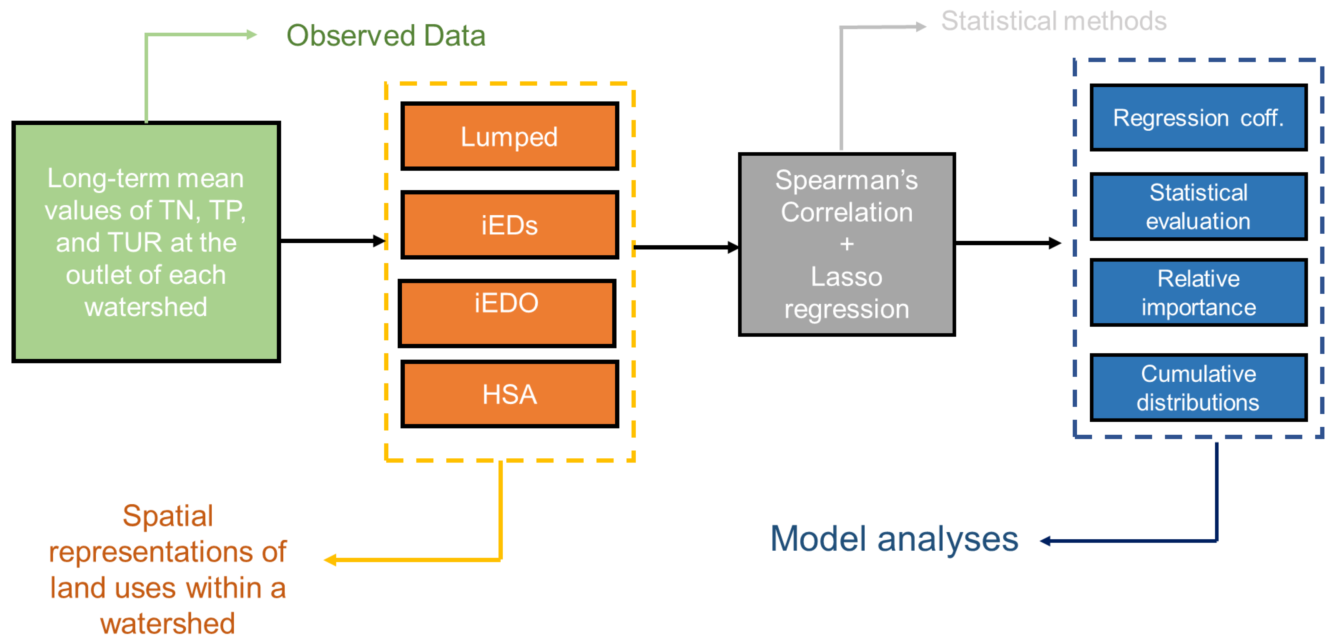
2.3. Model Development

The methodology framework developed in this paper is shown in Figure 2. This framework used observed data, including TN, TP, and TUR, at the outlet of each watershed and applied different land use metrics. A Spearman’s correlation model and a prediction model were then applied to assess the stream water quality at the outlet of each watershed using the selected metrics. The following sections provide detailed information on each method used in this study.

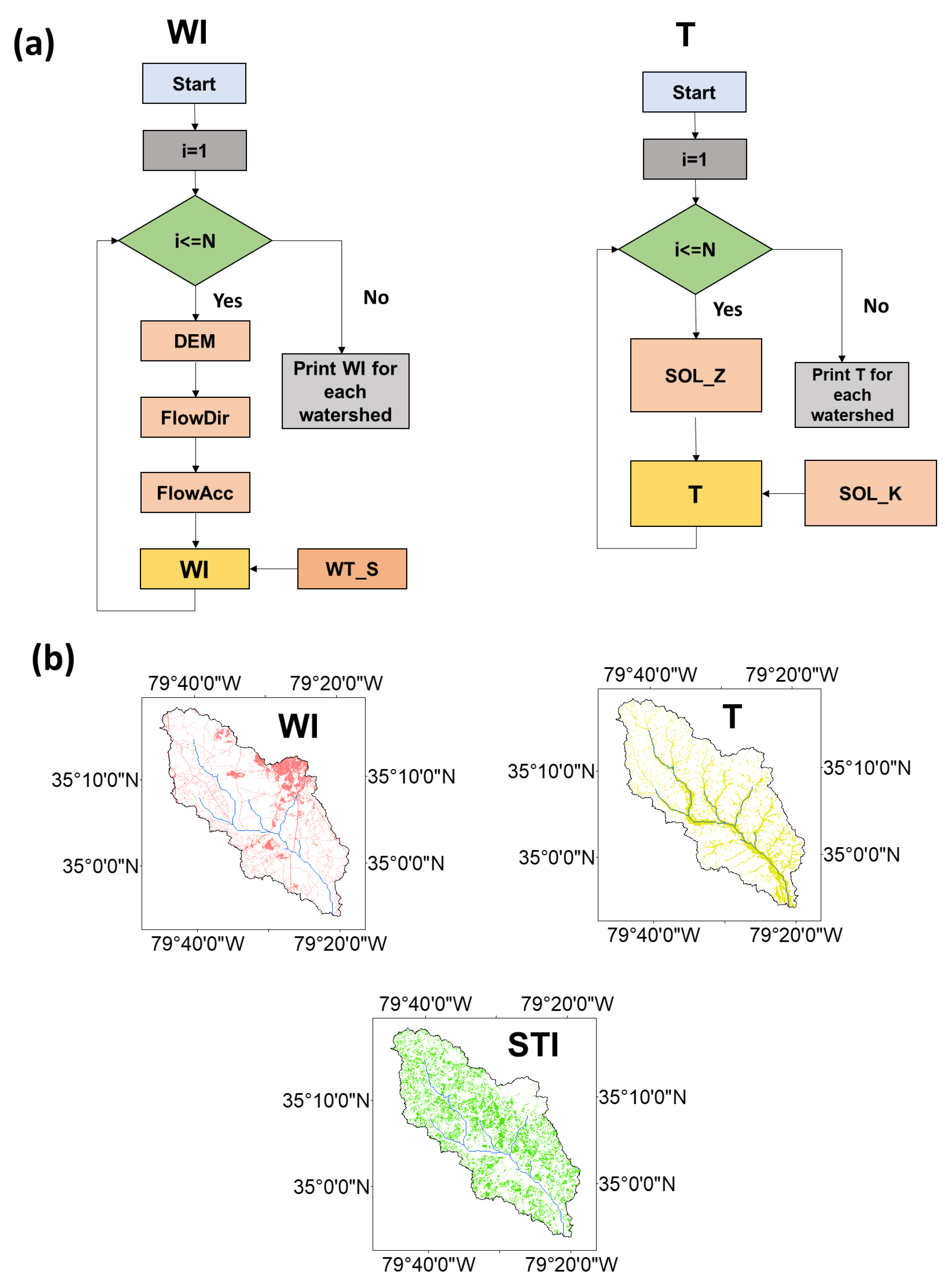
2.3.1. Inverse-Distance Weighted Metrics

In addition to the Lumped metric, where each land use cell in the watershed is given the same weight, the inverse-distance weighting (IDW) methods were used. This approach assigns more weight to land uses based on their proximity to certain key locations in the watershed. IDW was applied using two different methods. First, Inverse-Distance Weighted by Distance to the Outlet (iEDO). This method gives more weight to land uses closer to the watershed outlet as shown in Figure 3a. The second method is inverse distance weighted by distance to the stream (iEDs). This method gives more weight to land uses near the river or stream as shown in Figure 3b.
The main goal of IDW is to give more importance to land uses closer to the target (either the outlet or the stream). This can be mathematically represented using the following equation (Equation (1)):
% L U = i = 1 n I ( k ) W i i = 1 n W i 100
where I(k) is an indicator function that takes 1 if the i-th grid includes the evaluated land use and 0 otherwise; n is the total number of grids in the watershed.
Figure 4 shows an example of how the IDW was calculated based on Equation (1) for each watershed, focusing on either to the stream (IDWs) or the watershed outlet (IDWO). Each land use type within the watershed is evaluated individually; for example, when assessing the “URBAN” land use type, urban areas are assigned a value of 1, while all other land uses are given a value of 0. Following this, the IDW calculation is performed twice for each land use category—once from the stream (IDWs) and once from the watershed outlet (IDWO) to assess the spatial influence from both perspectives. This process is repeated for all 113 watersheds, with each land use type analyzed independently for its impact, ensuring a comprehensive evaluation of land use across the watershed areas.
The contribution of each i-th land use grid in a watershed to the final metric score is given by Equation (2), where Wi is the weighting for the i-th grid, di is the distance (either to the stream or to the watershed outlet), and p is the inverse-distance-weighting power (p ≤ 0). In this study, p was chosen to be −1 as suggested by [14] as it fits the data better compared to p = −0.5 or p = −2. In addition, p = −1 creates a smooth weighting transition near the stream compared to p = −2. Nevertheless, it was found that the weighting function was not smooth at the outlet. This may be related to the riparian zone near the outlet given more weight compared to lands farther from the outlet (Gregory et al. 1991 [29]).
W i = ( d + 1 ) p

2.3.2. Hydrological Sensitive Areas

Hydrological sensitive areas (HSAs) are areas within the watershed with significant potential for runoff [30]. Identifying these HSAs is crucial for recognizing critical source areas (the hot spots in the watershed) important for stakeholders and policymakers. Ref. [30] outlined various methods for delineating HSAs and emphasized the effectiveness of a threshold method by evaluating different Soil Transport Index (STI) values. Therefore, in this study, the Soil Transport Index (STI) was used, and different threshold values were evaluated.
The STI measures the likelihood that an area within the watershed generates saturation excess runoff [23,31,32]. The STI is determined using Equation (1), where α represents the upslope drainage area per unit contour length (m), β is the local surface slope (mm−1), and T is the soil transmissivity (m2/day).
S T I = ln α tan ( β ) ln ( T )
The term on the left-hand side of Equation (1) corresponds to the wetness index (WI). The WI is derived from the Digital Elevation Model (DEM). Using the DEM for each watershed, the watershed slope, flow direction, and flow accumulation was calculated to determine the WI for each area. (Figure 5a). The Least Squares Fitted Plane method [33] was employed to calculate the average slope of each watershed [34]. Soil transmissivity (T) was calculated using saturated hydraulic conductivity (SOL_K) and depth to a restrictive layer (SOL_Z), as discussed by [31]. Both SOL_K and SOL_Z were obtained from the Soil Survey Geographic (SSURGO) database and obtained from the U.S. Department of Agriculture (USDA) using the Soil Data Viewer tool version 6.2 (Figure 5a). SOL_K is the geometric mean of the saturated hydraulic conductivity across all soil layers within each watershed. The soil transmissivity was then integrated with the wetness index to determine the soil topographic index (STI) for each watershed. Figure 5b shows an example of the variations in the WI, T, and STI for a typical watershed.
In this study, a threshold value of ten was used to classify lands, where areas having STI values of ten or higher were designated as HSAs. This threshold was chosen because HSAs, on average, comprised 21% of the total area within each watershed. These findings align with previous research, which indicates that HSAs typically represent about 20% to 27% of a watershed [10,23]. Therefore, based on the 10 thresholds, only land uses within the HSAs are considered and studied to see their effects on the water quality at the outlet. In this study, the hydrologically sensitive areas are referred to as HSA in the results and discussion section.

2.3.3. Statistical Analysis

Statistical analyses were performed to examine the relationship between the long-term average water quality constituents TN, TP, and TUR at each watershed outlet and land use metric. Four distinct land use metrics were considered: HSA, iEDO, iEDs, and Lumped metrics. The goal was to determine which method most effectively represents the long-term behavior of water quality at the outlets of the watersheds. To achieve that, a range of Statistical tools was used, including covariate correlation analysis, LASSO regression, and relative importance analysis. To correlate land use metrics with the long-term average water quality of each watershed, Spearman’s rank correlation analysis was employed, as it is typically regarded as more robust and less sensitive to issues of non-normality and heteroscedasticity compared to Pearson’s correlation [35].
Seven land use variables were selected as independent (predictor) variables (Table 1), while the mean values of the water quality constituents (TN, TP, and TUR) were designated as dependent (response) variables. Given that the dependent variables did not follow a normal distribution, a Box–Cox transformation was applied to normalize the data [36]. Specifically, a log transformation was conducted to address the effects of skewness in the water quality variables. Each predictor variable was normalized to a mean of 0 and a variance of 1 across the watersheds. The dependent variables were averaged at the outlets of each watershed and analyzed to identify overall trends among the watersheds. A one-way ANOVA test revealed significant differences in water quality parameters among the selected watersheds, with a 95% confidence interval (α = 0.05; n = 113).

LASSO Regression

The least absolute shrinkage and selection operator (LASSO) regression approach was used to fit empirical models described by [37]. The LASSO was chosen as it recognizes model complexity and treats the predictor coefficients differentially. The LASSO method can effectively penalize large regression coefficients toward zero to minimize overfitting while selecting variables and estimating parameters for regression models [38]. Moreover, the LASSO outperforms stepwise regression, yielding improved results regarding goodness-of-fit metrics, such as the coefficient of determination and root mean square error (RMSE), for model evaluation [39]. Additionally, although the LASSO assumes linearity, it effectively selects key predictors and reduces multicollinearity, while nonlinear patterns can be captured through interaction terms or variable transformations [40].
The LASSO approach seeks to minimize the function given by Equation (5), where n is the number of data values, yi is the i-th dependent variable, α is the y-intercept coefficient, xi is the i-th independent variable, βi is the estimated value of the slope coefficient, and λ is a shrinkage factor that controls the complexity of the model.
min i = 1 n a + i = 1 j β i x i + λ i = 0 j β i
As the shrinkage coefficient, λ, approaches ∞, the complexity of the model increases. In this study, the optimal value of λ was determined using 10-fold cross validation method. During the cross-validation process, the data were divided into 10 folds. In each iteration, nine folds were used for training, while the remaining fold served as validation data. Various subsets of predictors were selected to fit the model based on the training data, and the resulting models were evaluated by computing the mean squared error (MSE) using the validation data. The fitted models were used to estimate the mean squared error (MSE) using the validation data. The value of λ within the minimum mean MSE values was selected for model fitting [40].
To analyze the relative importance of land use variables, the dominance analysis method using decomposition was applied [41]. In this method, R2 correlation-adjusted t-scores (CATs) are used to assess the relative significance of independent variables. This procedure was repeated for the four land use metrics: HSA, iEDO, iEDs, and Lumped.

Model Validation

A k-fold cross-validation approach was utilized to assess the models’ performance in ungauged watersheds [27]. In the initial run, 70% of the watersheds (n = 80) were randomly chosen for model calibration, while the remaining 30% (n = 33) were used for validation. This process was repeated 50 times to improve the reliability of the prediction results. These two steps enhance confidence in predicting water quality constituents in ungauged watersheds within the study area.
The performance of the final models for each mean water quality parameter was assessed using four different Statistical metrics. This included coefficient of determination (R2), Nash–Sutcliffe efficiency (NSE), root mean square error (RMSE), and percent bias (PBIAS). The performances of the final models were computed using Equations (5)–(8), where n is the total number of watersheds; Oi is the observed water quality variable at watershed i; O ¯ is the mean of the observed data; Pi is the predicted water quality constituent at watershed i; and p is the number of independent variables.
R 2 = i = 1 n ( O i O ¯ ) ( P i P ¯ ) i = 1 n ( O i O ¯ ) 2 i = 1 n ( P i P ¯ ) 2 2
N S E = 1 i = 1 n ( O i P i ) 2 i = 1 n ( O i O ¯ ) 2
R M S E = 1 n i = 1 n ( O i P i ) 2
P B I A S = i = 1 n ( P i O i ) × 100 i = 1 n O i
The coefficient of determination (R2) describes the degree to which the predicted data models the observed data (1.0 being the optimal value). NSE is the fitting of observed and predicted data in a 1:1 line and prediction becomes optimal as NSE approaches to 1.0. The RMSE represents the standard deviation of the residuals. PBIAS indicates underprediction (negative) and overprediction (positive) of the simulated data compared to the observed data, where zero is an optimal value. Empirical relationships are categorized by R2 values as weak (R2 ≤ 0.25), moderate (0.25 < R2 > 0.75), and strong (R2 ≥ 0.75) correlation based on the recommendation of [42].

3. Result

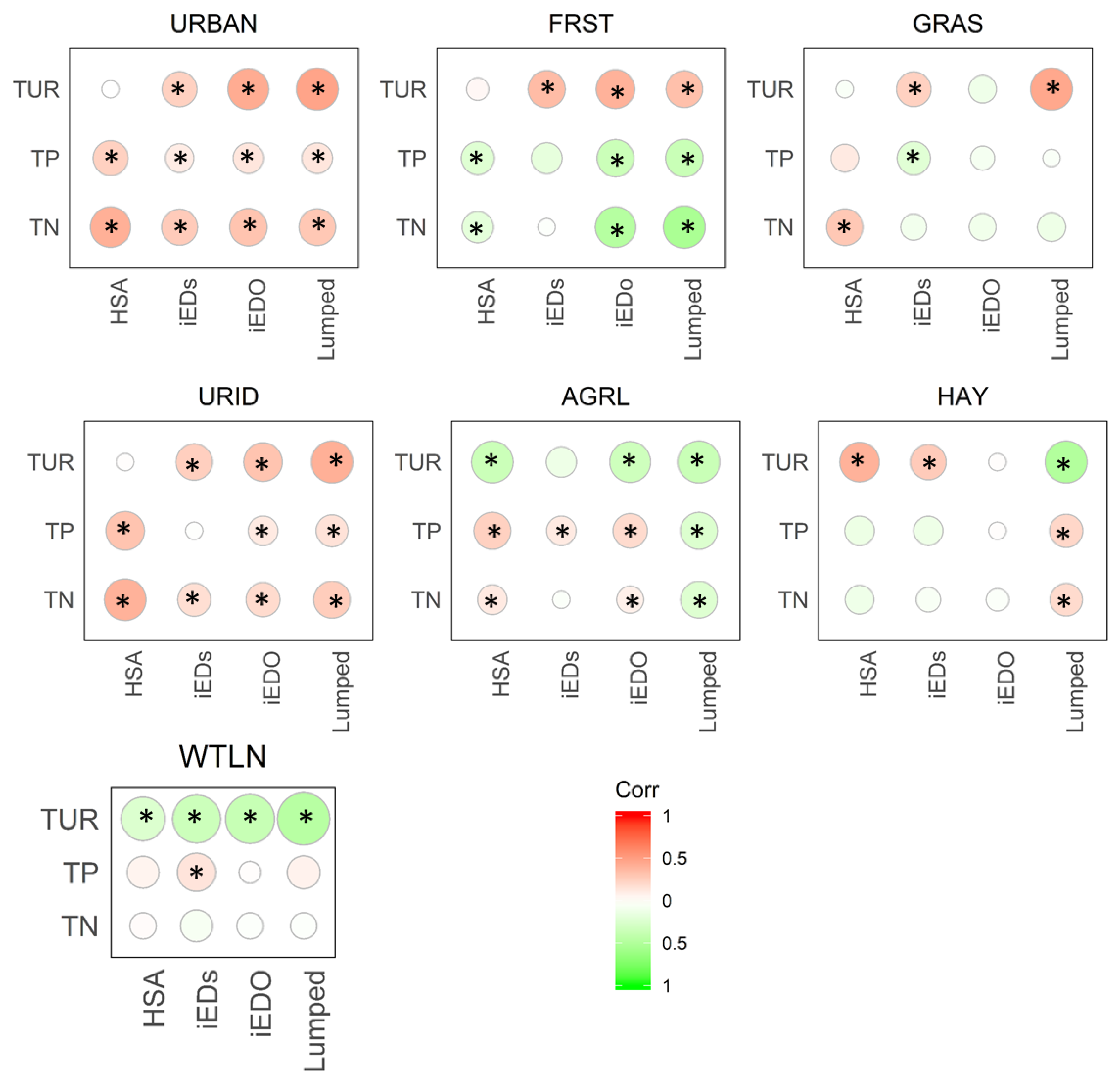
3.1. Visualization of Data and Correlations

Figure 6 presents the results of Spearman’s correlation analysis between mean stream water quality parameters (TN, TP, and TUR) and the land use metrics: Lumped, iEDO, iEDs, and HSA. The result indicates a significant positive correlation between TN and URBAN, URID, and AGRL lands for HSA and iEDO metrics. Additionally, there is a significant negative correlation between TN and FRST lands, while the correlation with other land uses at the HSA and iEDO metrics is negligible. Similar trends are observed with the iEDs metric, although the correlation between TN and FRST lands is insignificant.
Applying the Lumped metric, TN shows a positive correlation with URBAN and URID, a negative correlation with FRST and AGRL, and negligible correlations with other land use variables. The correlation analyses also reveal a significant positive correlation between TP and URBAN, URID, and AGRL lands, as well as a significant negative correlation between TP and FRST lands. Other correlations at the HSA and iEDO metrics are negligible. It is important to note that the correlation between TP, URID, and FRST is not significant in the iEDs metric. At the Lumped metric, significant positive correlations exist between TP and both URBAN and URID, while TP shows a significant negative correlation with FRST and AGRL lands, along with negligible correlations with other land uses within the selected watersheds.
For TUR values in streams, the analyses indicate that TUR is positively correlated with URBAN and negatively correlated with WTLN across all metrics. There are also positive correlations between TUR and URBAN, URID, and AGRL lands, alongside significant negative correlations with FRST and URID at the Lumped, iEDO, and iEDs metrics. However, the correlation between TUR and URID and FRST is not significant for the HSA metric. Furthermore, at the HSA and iEDs metrics, the analyses reveal a significant positive correlation between TUR and HAY lands in the study area.

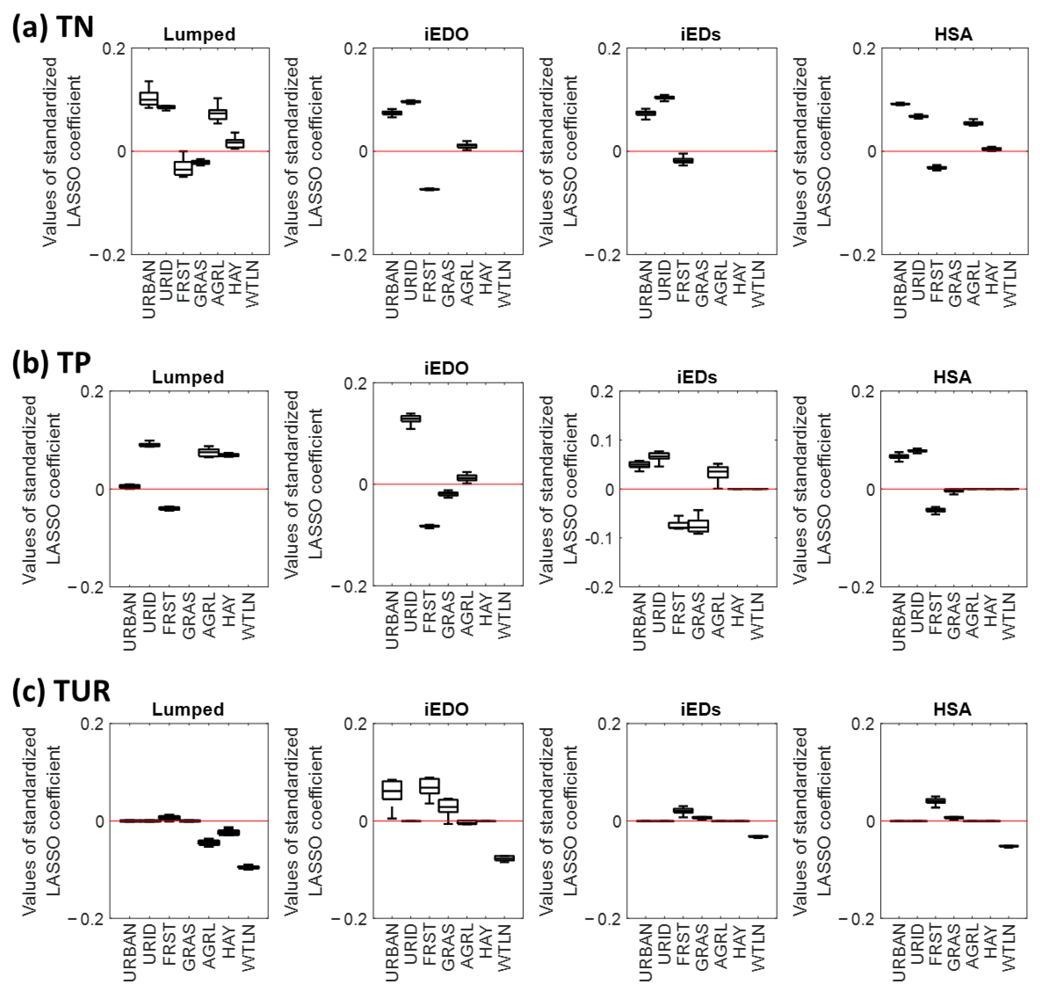
3.2. Relationship Between Water Quality Constituents and Land Use Variables

Figure 7a shows the LASSO regression coefficients of the mean TN concentration in streams and the land use evaluated at the four metrics: Lumped, iEDO, iEDS, and HSA. Applying the Lumped, iEDO, and HSA metrics shows that URBAN, URID, and AGRL lands have significant and positive effects on TN concentrations in streams. The findings indicate that URBAN and URID lands in watersheds have a greater impact on TN concentration compared to AGRL lands. For instance, applying the iEDO metric, a one percent increase in AGRL land in a watershed results in a 0.163 percent increase in TN concentration, whereas a one percent increase in URBAN land leads to a 0.448 percent increase in TN concentration. Conversely, FRST areas exhibit a negative effect on TN concentrations in streams. HAY and WTLN lands are Statistically insignificant and have no impact on TN concentration. The iEDs metric model excludes AGRL and GRAS lands while including URBAN and URID lands. Unlike the findings at the Lumped metric, evaluations of land use using the iEDO and iEDs metrics reveal that the impact on TN concentrations is greater from URID lands than URBAN lands (Figure 6).
Figure 7b presents the LASSO regression constants of land uses on TP in streams, assessed at the Lumped, iEDO, iEDS, and HSA metrics. All model results indicate that URBAN and URID lands positively and significantly influence TP concentrations in streams. Using the iEDO metric, a one percent increase in URBAN land elevates TP concentration by 0.0520 percent, while a one percent increase in URID land results in a 0.0625 percent increase in TP concentration. The HSA metric model shows similar outcomes to other metrics, with a few exceptions. First, the HSA metric model excludes AGRL land, which is significant in other models. Second, GRAS has a negative but minor impact on TP concentrations in streams.
The LASSO regression constants of land uses on TUR in streams are presented in Figure 7c. The iEDO metric model shows that URBAN, FRST, and GRAS lands positively impact TUR levels in streams, while only WTLN lands exert a negative influence on TUR values. The Lumped, iEDs, and HSA metrics models exclude URBAN land and only consider FRST, GRAS, and WTLN in contributing to TUR in a watershed. As with the iEDO metric model, the presence of FRST lands in HSAs reduces TUR concentrations in streams. The effects of FRST are significant, while the impacts of GRAS are less pronounced (Figure 7c). Overall, all metric modeling results suggest that FRST lands significantly increase TUR values in streams, while WTLN lands reduce these values.

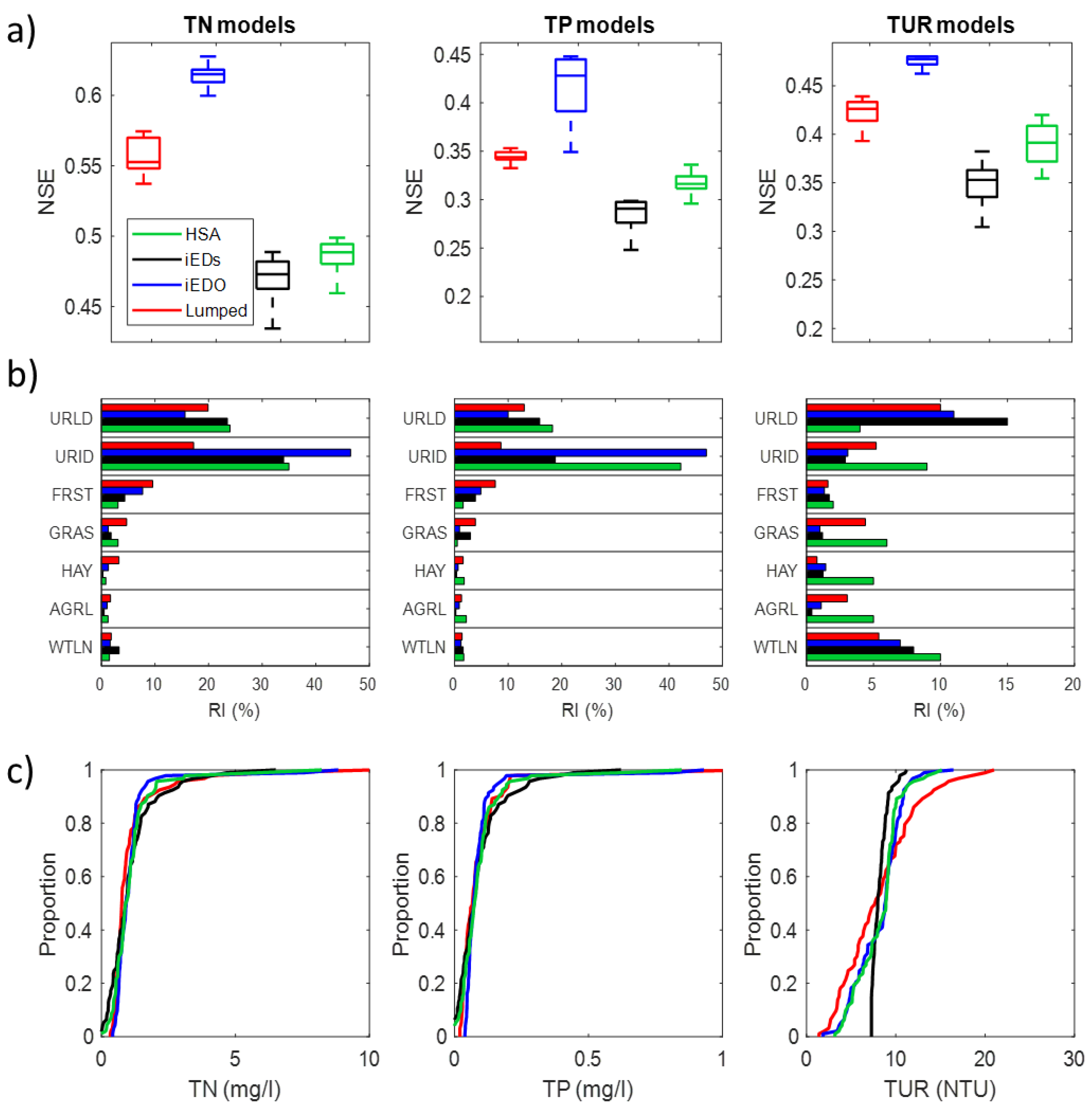
3.3. Model Performance

Figure 8 illustrates the predictive performance of the LASSO models using Lumped, HSA iEDO, and iEDs metrics (R2, PBIAS, and RMSE). The results indicate that the iEDO metric model outperforms the others, with R2 values ranging from 0.62 to 0.65. Additionally, the HSA and iEDs metrics models demonstrate similar levels of accuracy based on the mean values of RMSE and PBIAS. Overall, the R2 values show that the models explain approximately 45% of the variability in TN, 32% in TP, and 38% in TUR.
Figure 9 presents the NSE values, relative importance analysis, and cumulative distribution of TN, TP, and TUR across the selected watersheds. The NSE values indicate that the evaluation of land uses at the iEDO metric performs better than the other models. The performance of iEDO is followed by the Lumped, iEDs, and HSA metrics for all water quality constituents (Figure 9a). The relative importance of each predictor was determined from 50 runs of each model using the dominance analysis method (Figure 9b). The predictions from these models are significantly influenced by the URBAN and URID land types. The importance of each variable has been normalized to facilitate comparison between the models, and the magnitude of predictor importance varies among them.
For TN, the evaluation at the iEDO metric indicates that URID exerts the greatest influence on TN concentration, followed by URBAN and FRST lands (Figure 9b). Conversely, the most important predictors for TUR are URBAN and WTLN lands. These findings suggest that URBAN and WTLN are the primary variables affecting the spatial variability of TUR in the streams within the study area. The HSA model reveals that the variability in TN is mainly explained by URID, which has a relative importance of 32%, followed by URBAN at 17%.
All models exhibit similar cumulative mean predictions for TN, TP, and TUR distributions (Figure 9c). These models provide robust estimates for low TN, TP, and TUR values (almost 75% of the samples) but tend to underpredict TN, TP, and TUR for high values concentrations (almost 25% of the samples).

4. Discussion

The significant impacts of URBAN and URID land on TN concentration are understandable, especially when evaluating the land uses using the iEDO metric. The high TN concentration from the URBAN and URID (especially closer to a watershed outlet) can be attributed to fertilizer use on lawns and the presence of animal waste [43,44,45]. Another possible reason for the higher TN concentration in urban areas is legacy nitrogen—residual nitrogen from past agricultural activities accumulated in soil and groundwater over time. Many URBAN lands in the study area were converted from agricultural land to low-density urban lands [11]. Such effects might act as a long-term source of mineralization and leaching to waterways. This may result in high TN concentration in the streams. In ref. [46], URBAN lands were the main source of TN in the Wheeler Lake watershed in northern Alabama and southern Tennessee in the U.S.
Similarly, Ref. [47] observed comparable results in the Lake Calumet Basin in the Greater Chicago area. Ref. [48] highlighted a negative correlation between forested areas (FRST) and TN concentrations in streams within the Boston metropolitan area in eastern Massachusetts. The TP modeling results agree with the results found in previous studies. Refs. [49,50] identified AGRL and URBAN land as the primary sources of TP concentrations in streams, specifically in the Portland metropolitan area, Oregon, and the Xitiaoxi River Basin, China, respectively. Ref. [48] showed that forested areas significantly reduced phosphorus concentrations in rivers around the Boston metropolitan area in eastern Massachusetts.
Although urbanization is deemed to be the main reason for stream water quality degradation, most of the previous studies did not delineate the impact of different urbanization types on stream water quality. The findings of this study showed that URID lands impacted the quality of the stream water. The results at Lumped, iEDO, iEDS, and HSA metrics suggested that URBAN plays a significant role in increasing TN and TP concentrations in streams. The iEDO and HSA metrics models also showed that URID is the most important variable affecting TN and TP concentrations in the streams. The modeling results also showed that AGRL land increased, while forest reduced TN and TP concentrations with different significant values.
Additionally, a significant positive correlation between turbidity (TUR) and hay lands (HAY) in the HSA and iEDs metrics was observed and suggested that hay land concentration is linked to elevated turbidity, likely due to agricultural runoff or soil disturbance. On the other hand, the Lumped metric, which assigns equal weight to all land uses, shows a significant negative correlation, indicating that other watershed factors may overshadow hay land effects. Moreover, the agricultural lands (ARGL) significantly increase total nitrogen (TN) concentrations in streams, as shown by the Lumped, iEDO, and HSA metrics, likely due to fertilizer runoff, livestock waste, and other agricultural practices. The iEDS metric shows no effect, possibly because it emphasizes proximity to streams; if agricultural lands are more dispersed, their impact on TN may be less noticeable. Similarly, agricultural lands significantly contribute to total phosphorus (TP) concentrations in the Lumped, iEDO, and iEDS metrics, reinforcing the role of fertilizer and livestock waste in phosphorus runoff. However, the HSA metric shows no effect, possibly because agricultural lands are not concentrated in hydrologically sensitive areas within the study area.
The findings from this study support the hypothesis that evaluating the land uses at iEDO, iEDs, and HSA metrics is more meaningful compared to just giving the same weight to all land uses within a watershed (Lumped method). This was clear by looking at the evaluation statistics between the different metric models. These findings may facilitate the management strategies for watershed protection and water conservation. Watershed managers can focus on a specific location in the watershed (areas closer to the streams or the outlets) or focus only on the HSAs in a watershed rather than the whole watershed to implement best management practices (BMPs) for improving water quality. To illustrate, implementing BMPs is important to control nonpoint source pollution from URBAN and URID lands. Nevertheless, it is not feasible to implement BMPs in all agricultural or urban areas within a watershed. Instead, BMPs may be applied in specific locations within the watershed to optimize available resources. Watershed managers should target AGRL lands and URBAN land within HSAs to reduce TN and TP concentration in streams.
Additionally, in order to reduce TN and TP concentration in streams, URID closer to streams should be strategically protected. Furthermore, the identified HSAs within a watershed should be safeguarded from urban development to preserve overall watershed health. The findings of this study would also help arrange different parts of a watershed for conservation efforts as well as direct urban growth from the sensitive areas within a watershed.
While this study provides valuable insights into the impact of different land uses on stream water quality, there are some limitations to consider. The analysis is based on long-term mean average water quality parameters, and thus, temporal variations in land use and water quality were not included. Future studies could examine the temporal dynamics of land use change and its influence on stream water quality, including seasonal and annual variations. This would provide a more comprehensive understanding of how different land use metrics affect water quality over time.

5. Conclusions

The main objective of this study was to evaluate the effects of land use alteration, especially when including different land use metrics on stream water quality. A series of LASSO models using four different land use metrics were developed at the outlet of 113 watersheds to enhance the understanding of how the land use location and the hotspots within a watershed alter stream water quality. Overall, better-fit LASSO models were developed when land uses were evaluated using the iEDO, iEDs, and HSA metrics than the Lumped model metric. Additionally, the models developed using the iEDO, iEDs, and HSA metrics provided deeper mechanistic insights into the relationship between land use patterns and stream water quality within a watershed.
The land use approaches based on IDW and HSA helped to show the effects of industrial lands. These approaches highlighted how different parts of a watershed affected the stream water quality. The findings confirmed the hypothesis that not only does the percentage of urbanization in a watershed influence water quality, but the type of urban development and the location of land use also play crucial roles. These findings can have important implications for watershed managers, which may assist in protecting stream water quality through advanced management practices. Specifically, there are many methods of land use measures that stakeholders can use to direct urbanization development. Such land use measures may include riparian zones and wetland protection. Future studies should focus on examining riparian zones to determine whether they yield improved modeling results compared to those presented in this study.

Author Contributions

Conceptualization, A.O.A.; Methodology, A.O.A.; Validation, A.O.A.; Formal analysis, A.O.A.; Writing—original draft, A.O.A.; Writing—review & editing, A.O.A., A.K.M. and A.A.K.; Supervision, A.K.M. and A.A.K.; Funding acquisition, A.A.K. All authors have read and agreed to the published version of the manuscript.

Funding

This research received no external funding.

Data Availability Statement

The raw data supporting the conclusions of this article will be made available by the authors on request.

Acknowledgments

This publication is based on a chapter from the first author’s doctoral thesis “Quantifying the Role of Climate and Watershed Characteristics on Surface Water Quality in Southeast Atlantic region of the US” submitted to Clemson University in partial fulfillment of the requirements for the PhD degree.

Conflicts of Interest

The authors declare no conflicts of interest.

References

  1. Abdul-Aziz, O.I.; Ishtiaq, K.S.; Tang, J.; Moseman-Valtierra, S.; Kroeger, K.D.; Gonneea, M.E.; Mora, J.; Morkeski, K. Environmental controls, emergent scaling, and predictions of greenhouse gas (GHG) fluxes in coastal salt marshes. J. Geophys. Res. Biogeosci. 2018, 123, 2234–2256. [Google Scholar] [CrossRef]
  2. Allan, J.D. Landscapes and riverscapes: The influence of land use on stream ecosystems. Annu. Rev. Ecol. Evol. Syst. 2004, 35, 257–284. [Google Scholar] [CrossRef]
  3. Baker, A. Land use and water quality. In Encyclopedia of Hydrological Sciences; Wiley: Hoboken, NJ, USA, 2006. [Google Scholar]
  4. Walsh, C.J.; Webb, J.A. Interactive effects of urban stormwater drainage, land clearance, and flow regime on stream macroinvertebrate assemblages across a large metropolitan region. Freshw. Sci. 2016, 35, 324–339. [Google Scholar] [CrossRef]
  5. Tong, S.T.Y.; Chen, W. Modeling the relationship between land use and surface water quality. J. Environ. Manag. 2002, 66, 377–393. [Google Scholar] [CrossRef]
  6. Marzin, A.; Archaimbault, V.; Belliard, J.; Chauvin, C.; Delmas, F.; Pont, D. Ecological assessment of running waters: Do macrophytes, macroinvertebrates, diatoms and fish show similar responses to human pressures? Ecol. Indic. 2012, 23, 56–65. [Google Scholar] [CrossRef]
  7. Junior, R.F.V.; Varandas, S.G.P.; Pacheco, F.A.L.; Pereira, V.R.; Santos, C.F.; Cortes, R.M.V.; Fernandes, L.F.S. Impacts of land use conflicts on riverine ecosystems. Land Use Policy 2015, 43, 48–62. [Google Scholar] [CrossRef]
  8. Johnson, S.L.; Ringler, N.H. The response of fish and macroinvertebrate assemblages to multiple stressors: A comparative analysis of aquatic communities in a perturbed watershed (Onondaga Lake, NY). Ecol. Indic. 2014, 41, 198–208. [Google Scholar] [CrossRef]
  9. Siqueira, T.d.S.; Pessoa, L.A.; Vieira, L.; Cionek, V.d.M.; Singh, S.K.; Benedito, E.; do Couto, E.V. Evaluating land use impacts on water quality: Perspectives for watershed management. Sustain. Water Resour. Manag. 2023, 9, 192. [Google Scholar] [CrossRef]
  10. Qiu, Z.; Kennen, J.G.; Giri, S.; Walter, T.; Kang, Y.; Zhang, Z. Reassessing the relationship between landscape alteration and aquatic ecosystem degradation from a hydrologically sensitive area perspective. Sci. Total Environ. 2019, 650, 2850–2862. [Google Scholar] [CrossRef]
  11. Alnahit, A.O.; Mishra, A.K.; Khan, A.A. Quantifying climate, streamflow, and watershed control on water quality across Southeastern US watersheds. Sci. Total Environ. 2020, 739, 139945. [Google Scholar] [CrossRef]
  12. Lee, J.W.; Park, S.R.; Lee, S.W. Effect of Land Use on Stream Water Quality and Biological Conditions in Multi-Scale Watersheds. Water 2023, 15, 4210. [Google Scholar] [CrossRef]
  13. Ullah, K.A.; Jiang, J.; Wang, P. Land use impacts on surface water quality by statistical approaches. Glob. J. Environ. Sci. Manag. 2018, 4, 231–250. [Google Scholar]
  14. King, R.S.; Baker, M.E.; Whigham, D.F.; Weller, D.E.; Jordan, T.E.; Kazyak, P.F.; Hurd, M.K. Spatial considerations for linking watershed land cover to ecological indicators in streams. Ecol. Appl. 2005, 15, 137–153. [Google Scholar] [CrossRef]
  15. Williams, N.S.G.; Morgan, J.W.; McDonnell, M.J.; Mccarthy, M.A. Plant traits and local extinctions in natural grasslands along an urban–rural gradient. J. Ecol. 2005, 93, 1203–1213. [Google Scholar] [CrossRef]
  16. Peterson, E.E.; Sheldon, F.; Darnell, R.; Bunn, S.E.; Harch, B.D. A comparison of spatially explicit landscape representation methods and their relationship to stream condition. Freshw. Biol. 2011, 56, 590–610. [Google Scholar] [CrossRef]
  17. Paringit, E.C.; Nadaoka, K. Sediment yield modelling for small agricultural catchments: Land-cover parameterization based on remote sensing data analysis. Hydrol. Process. 2003, 17, 1845–1866. [Google Scholar] [CrossRef]
  18. Sweeney, B.W.; Bott, T.L.; Jackson, J.K.; Kaplan, L.A.; Newbold, J.D.; Standley, L.J.; Hession, W.C.; Horwitz, R.J. Riparian deforestation, stream narrowing, and loss of stream ecosystem services. Proc. Natl. Acad. Sci. USA 2004, 101, 14132–14137. [Google Scholar] [CrossRef]
  19. Baker, A.; Cumberland, S.A.; Bradley, C.; Buckley, C.; Bridgeman, J. To what extent can portable fluorescence spectroscopy be used in the real-time assessment of microbial water quality? Sci. Total Environ. 2015, 532, 14–19. [Google Scholar] [CrossRef]
  20. Sliva, L.; Williams, D.D. Buffer zone versus whole catchment approaches to studying land use impact on river water quality. Water Res. 2001, 35, 3462–3472. [Google Scholar] [CrossRef]
  21. Townsend, C.R.; Dolédec, S.; Norris, R.; Peacock, K.; Arbuckle, C. The influence of scale and geography on relationships between stream community composition and landscape variables: Description and prediction. Freshw. Biol. 2003, 48, 768–785. [Google Scholar] [CrossRef]
  22. Sweeney, B.W.; Newbold, J.D. Streamside forest buffer width needed to protect stream water quality, habitat, and organisms: A literature review. J. Am. Water Resour. Assoc. 2014, 50, 560–584. [Google Scholar] [CrossRef]
  23. Giri, S.; Qiu, Z.; Zhang, Z. Assessing the impacts of land use on downstream water quality using a hydrologically sensitive area concept. J. Environ. Manag. 2018, 213, 309–319. [Google Scholar] [CrossRef]
  24. Qiu, Z.; Hall, C.; Drewes, D.; Messinger, G.; Prato, T.; Hale, K.; Van Abs, D. Hydrologically sensitive areas, land use controls, and protection of healthy watersheds. J. Water Resour. Plan. Manag. 2014, 140, 04014011. [Google Scholar] [CrossRef]
  25. Hewlett, J.D. Principles of Forest Hydrology; University of Georgia Press: Athens, GA, USA, 1982. [Google Scholar]
  26. Homer, C.G.; Fry, J.A.; Barnes, C.A. The National Land Cover Database; US Geological Survey: Reston, VA, USA, 2012. [Google Scholar]
  27. Alnahit, A.O.; Mishra, A.K.; Khan, A.A. Stream water quality prediction using boosted regression tree and random forest models. Stoch. Environ. Res. Risk Assess. 2022, 36, 2661–2680. [Google Scholar] [CrossRef]
  28. Hirsch, R.M.; De Cicco, L.A. User Guide to Exploration and Graphics for RivEr Trends (EGRET) and DataRetrieval: R Packages for Hydrologic Data; US Geological Survey: Reston, VA, USA, 2015. [Google Scholar]
  29. Gregory, S.V.; Swanson, F.J.; McKee, W.A.; Cummins, K.W. An ecosystem perspective of riparian zones. Bioscience 1991, 41, 540–551. [Google Scholar] [CrossRef]
  30. Qiu, Z. Assessing critical source areas in watersheds for conservation buffer planning and riparian restoration. Environ. Manag. 2009, 44, 968–980. [Google Scholar] [CrossRef]
  31. Buchanan, B.P.; Fleming, M.; Schneider, R.L.; Richards, B.K.; Archibald, J.; Qiu, Z.; Walter, M.T. Evaluating topographic wetness indices across central New York agricultural landscapes. Hydrol. Earth Syst. Sci. 2014, 18, 3279–3299. [Google Scholar] [CrossRef]
  32. Walter, M.T.; Steenhuis, T.S.; Mehta, V.K.; Thongs, D.; Zion, M.; Schneiderman, E. Refined conceptualization of TOPMODEL for shallow subsurface flows. Hydrol. Process. 2002, 16, 2041–2046. [Google Scholar] [CrossRef]
  33. Horn, B.K.P. Hill shading and the reflectance map. Proc. IEEE 1981, 69, 14–47. [Google Scholar] [CrossRef]
  34. Seibert, J.; McGlynn, B.L. A new triangular multiple flow direction algorithm for computing upslope areas from gridded digital elevation models. Water Resour. Res. 2007, 43, W04501. [Google Scholar] [CrossRef]
  35. Hauke, J.; Kossowski, T. Comparison of values of Pearson’s and Spearman’s correlation coefficients on the same sets of data. Quaest. Geogr. 2011, 30, 87–93. [Google Scholar] [CrossRef]
  36. Box, G.E.P.; Cox, D.R. An analysis of transformations. J. R. Stat. Soc. Series B Stat. Methodol. 1964, 26, 211–243. [Google Scholar] [CrossRef]
  37. Bardsley, W.E.; Vetrova, V.; Liu, S. Toward creating simpler hydrological models: A LASSO subset selection approach. Environ. Model. Softw. 2015, 72, 33–43. [Google Scholar] [CrossRef]
  38. Camilo, D.C.; Lombardo, L.; Mai, P.M.; Dou, J.; Huser, R. Handling high predictor dimensionality in slope-unit-based landslide susceptibility models through LASSO-penalized Generalized Linear Model. Environ. Model. Softw. 2017, 97, 145–156. [Google Scholar] [CrossRef]
  39. Hammami, D.; Lee, T.S.; Ouarda, T.B.M.J.; Lee, J. Predictor selection for downscaling GCM data with LASSO. J. Geophys. Res. Atmos. 2012, 117, D17116. [Google Scholar] [CrossRef]
  40. Tibshirani, R. Regression shrinkage and selection via the lasso. J. R. Stat. Soc. Series B Stat. Methodol. 1996, 58, 267–288. [Google Scholar] [CrossRef]
  41. Zuber, V.; Strimmer, K. High-dimensional regression and variable selection using CAR scores. Stat. Appl. Genet. Mol. Biol. 2011, 10. [Google Scholar] [CrossRef]
  42. Hair, J.F.; Ringle, C.M.; Sarstedt, M. Partial least squares structural equation modeling: Rigorous applications, better results and higher acceptance. Long Range Plann. 2013, 46, 1–12. [Google Scholar] [CrossRef]
  43. Kaushal, S.S.; Groffman, P.M.; Band, L.E.; Shields, C.A.; Morgan, R.P.; Palmer, M.A.; Belt, K.T.; Swan, C.M.; Findlay, S.E.G.; Fisher, G.T. Interaction between urbanization and climate variability amplifies watershed nitrate export in Maryland. Environ. Sci. Technol. 2008, 42, 5872–5878. [Google Scholar] [CrossRef]
  44. Law, N.; Band, L.; Grove, M. Nitrogen input from residential lawn care practices in suburban watersheds in Baltimore County, MD. J. Environ. Plan. Manag. 2004, 47, 737–755. [Google Scholar] [CrossRef]
  45. Paul, M.J.; Meyer, J.L. Streams in the urban landscape. Annu. Rev. Ecol. Syst. 2001, 32, 333–365. [Google Scholar] [CrossRef]
  46. Pratt, B.; Chang, H. Effects of land cover, topography, and built structure on seasonal water quality at multiple spatial scales. J. Hazard. Mater. 2012, 209, 48–58. [Google Scholar] [CrossRef] [PubMed]
  47. Wilson, C.; Weng, Q. Assessing surface water quality and its relation with urban land cover changes in the Lake Calumet Area, Greater Chicago. Environ. Manag. 2010, 45, 1096–1111. [Google Scholar] [CrossRef]
  48. Tu, J. Spatially varying relationships between land use and water quality across an urbanization gradient explored by geographically weighted regression. Appl. Geogr. 2011, 31, 376–392. [Google Scholar] [CrossRef]
  49. Tsegaye, T.; Sheppard, D.; Islam, K.R.; Tadesse, W.; Atalay, A.; Marzen, L. Development of chemical index as a measure of in-stream water quality in response to land-use and land cover changes. Water Air Soil. Pollut. 2006, 174, 161–179. [Google Scholar] [CrossRef]
  50. Wan, R.; Cai, S.; Li, H.; Yang, G.; Li, Z.; Nie, X. Inferring land use and land cover impact on stream water quality using a Bayesian hierarchical modeling approach in the Xitiaoxi River Watershed, China. J. Environ. Manag. 2014, 133, 1–11. [Google Scholar] [CrossRef]
Figure 1. Selected watersheds in three South Atlantic States in the USA.
Water 17 00849 g001
Figure 2. The methodology framework developed in this study.
Water 17 00849 g002
Figure 3. An example of two IDW methods in the spatial analysis of land use: (a) distance to the watershed outlet and (b) distance to the stream. The colors indicate a gradient of distance values, ranging from near (red) to far away (blue) relative to the watershed outlet or stream [14].
Water 17 00849 g003
Figure 4. An example illustrating the calculation of IDW for each watershed, whether at the stream or the watershed outlet. Each land use type was evaluated individually; for instance, if URBAN is assessed in the watershed, it is given a value of 1, and all other land uses are assigned a value of 0. Note: The same analysis was performed for the other 113 watersheds.
Water 17 00849 g004
Figure 5. (a) Flowcharts showing the steps for calculating the wetness index (WI) and soil transmissivity (T) for each watershed in the study. (b) An example illustrating the spatial distribution of the wetness index (WI), soil transmissivity (T), and soil topographic index (STI) within a specific watershed. Note: The STI was calculated for each watershed, where N signifies the total number of evaluated watersheds. In this case, N = 113.
Water 17 00849 g005
Figure 6. Spearman’s correlation matrix for water quality parameters and land use in watersheds. [Note: * indicates the correlation is Statistically significant (p < 0.05)].
Water 17 00849 g006
Figure 7. Standardized LASSO regression coefficients for land use predictors of mean (a) TN concentrations, (b) TP concentrations, and (c) TUR concentrations. Coefficients were derived from 50 runs of the LASSO model. The lines in the box indicate the medians of 50 runs.
Water 17 00849 g007
Figure 8. Results of Statistical evaluation for (a) TN, (b) TP, and (c) TUR models across the selected watersheds using the LASSO with 50 runs for different landscape representations: Lumped, HSA, iEDO, and iEDs. The lines in the box indicate the medians of 50 runs.
Water 17 00849 g008
Figure 9. (a) NSE comparison for TN, TP, and TUR between the four different landscape representations (based on the validation subsets), Lumped, HSA, iEDO, and iEDs, as a result of the 50 runs; (b) the relative influence of predictors for the TN, TP, and TUR models based on the dominance analysis method; and (c) cumulative distributions of TN, TP, and TUR predicted by the 50 runs of the LASSO model.
Water 17 00849 g009
Table 1. Definitions and characteristics of land uses in the evaluated watersheds. The land use data were obtained from the National Land Cover Database (NLCD) for the year 2011. The percentages and statistics for the investigated watersheds in the study area were generated using ArcGIS software version 10.7.
Land Use
Type
DefinitionMeanStandard DeviationMinimum25th Percentile50th Percentile75th PercentileMaximum
URBAN (%)Total percent of urban land use10.56.92.15.18.314.533.6
URID (%)Total percent industrial urban land use7.49.70.42.02.89.743.0
FRST (%)Total percent forest land use1.31.80.00.40.71.38.1
GRAS (%)Total percentage of grassland use (e.g., Range-Brush)41.515.812.830.040.453.781.5
HAY (%)Total percent hay land (Range-Brush and Range-Grasses)11.26.31.27.29.615.324.7
AGRL (%)Total percent agricultural land use18.810.50.711.617.522.553.6
WTLN (%)Total percent wetland land use8.411.80.00.82.713.566.3
Disclaimer/Publisher’s Note: The statements, opinions and data contained in all publications are solely those of the individual author(s) and contributor(s) and not of MDPI and/or the editor(s). MDPI and/or the editor(s) disclaim responsibility for any injury to people or property resulting from any ideas, methods, instructions or products referred to in the content.

