Abstract
In order to ensure the smooth progress of foundation pit engineering, it is necessary to identify and control the seepage risk. At present, there are few research studies and applications on the seepage risk assessment of foundation pits, and the optimization of curtain depth and the interrelation and optimal combination of design variables are rarely considered in the optimization design of foundation pit dewatering scheme based on the objective function method. According to the geological and hydrogeological conditions of the research area, a mathematical model for optimizing foundation pit dewatering was established. The model takes the minimum total dewatering cost as the objective function and comprehensively considers decision-making variables. Additionally, it also takes into account constraints such as the drawdown depth of the water level in a single well and the pumping flow rate of a single well. The calculation results indicate that the errors between the measured water levels and the simulated water levels are within ±3.5%, suggesting that the parameter inversion results are effective. The horizontal and vertical permeability coefficients of the phreatic aquifer are 3.0 m/d and 0.45 m/d, respectively, and the horizontal and vertical permeability coefficients of confined aquifer are 10.28 m/d and 1.25 m/d, respectively. The horizontal and vertical permeability coefficients of the confined aquifer are 10.28 m/d and 1.25 m/d, respectively. Nine different excavation dewatering schemes that curtain depths of 66 m, 61 m, and 56 m were designed, and the optimal excavation dewatering scheme was determined by comparing the total dewatering cost. This scheme has the advantages of shortening the dewatering time, reducing the impact of foundation pit dewatering on the surrounding environment, and saving the total cost of dewatering. The research results provide a relevant decision-making basis for managers.
1. Introduction
In recent years, with the acceleration of urbanization, the demand for large buildings has increased, and, as the main underground structure of large buildings, various foundation pit projects have emerged [1]. The advancement of deep and dense configuration of foundation pits has become an inevitable trend, and the requirements of foundation pit construction are becoming increasingly strict. Foundation pit dewatering is a key aspect of this process. During foundation pit excavation, the pore–water pressure in the soil constantly changes. This change disrupts the original mechanical equilibrium and may trigger adverse geological phenomena such as piping and suffusion. Moreover, it can cause settlement of the ground in the vicinity and adjacent structures, as well as the wastage of groundwater resources [2,3,4]. To prevent the occurrence of geological disasters mentioned above and ensure the safety of the construction process, the optimization design of the excavation system is crucial [5,6].
The design methods of foundation pit dewatering mainly include (1) the numerical simulation method, (2) large well method, and (3) multi-objective optimization approach [7]. Among these, the multi-objective optimization approach focuses on minimizing economic costs or reducing environmental impact while determining other parameter values to optimally achieve design objectives, though it is subject to constraints such as well depth for water descent and the production of each well. To precisely calculate the dimensions of the pit and the distribution of the hydraulic head outside the pit, the numerical simulation method emerges as an effective approach for resolving dewatering or related problems [8,9,10,11]. Yan Xu et al. took the minimum total drainage as the objective function and the water level at the control points as the primary constraint and optimize the design of the sinking depth of the tube well cluster in the underground tunnel [8]. Dan Yu et al. took the minimization of the maximum value of the drawdown rate of the water level at the control points as the objective function and optimized the design using the optimization toolbox in MATLAB8.0 software under the condition of achieving the designed drawdown rate of the groundwater level at the control points [7]. Nianqing Zhou et al. used the numerical simulation method to calculate the drawdown rate of the Xujiahui subway station and the distribution of hydraulic heads outside of the pit to the maximum extent to achieve the design purpose [12]. He Guo-ping et al. used the groundwater numerical simulation software, FEFLOW7.0, to establish hydro-geological unit models and predicted the groundwater system in the downstream reach of the Yellow River, providing a theoretical basis for the rational exploitation of underground water resources [13]. Iván Alhama et al. derived the dimensionless groups for the solutions of anisotropic seepage through discriminative non-dimensionalization of the governing equations and boundary conditions. They studied three different cases of finite domains, verified the results using numerical simulations, and presented new type curves [14]. In the current field of dewatering design, many scholars have carried out abundant research. Most of the scholars use multi-objective optimization method in the design of pit descending, taking the minimization of total drainage, groundwater level control, and minimization of ground settlement as the objective functions. This research idea effectively solves many technical problems in the process of pit dewatering to a certain extent and plays a positive role in guaranteeing the smooth progress of engineering construction and the stability of the surrounding environment. However, it is worth noting that there are still obvious research gaps. There is a lack of research related to minimizing the total cost of dewatering as the objective function. In practical engineering, cost control is a crucial aspect, which not only relates to the economic benefits of the project but also affects the rational utilization of resources. The lack of in-depth research on minimizing the total cost of dewatering makes it difficult to find the optimal balance between technical feasibility and economic rationality when making decisions on actual projects. In addition, designers usually adopt overly conservative parameters when it comes to ensuring structural safety. Although this practice can minimize risks from a safety perspective, it brings about an unnecessary increase in construction costs. Overly conservative parameter selection means that the use of materials and equipment configuration exceeds the actual demand, resulting in the waste of resources and unreasonable expenditure of funds. This not only poses a challenge to the cost control of individual projects but is also not conducive to the improvement in resource utilization efficiency and sustainable development of the entire construction industry from a macro perspective. Therefore, how to optimize the parameter selection and reduce the construction cost under the premise of guaranteeing structural safety, while carrying out the research with the minimization of the total cost of dewatering as the objective function, is an important issue that needs to be solved in the field of foundation pit dewatering design at present.
This article takes the Haitai Tunnel shield tunneling project as an example and establishes a mathematical model for pit optimization using the multi-objective optimization method. The objective function is to minimize the total cost, considering decision variables such as well group depth, location, quantity, pumping rate, pumping time, filter length and location, and impervious curtain depth, combined with constraints on water level drop depth, settlement amount, and pumping rate of a single well. Finally, FEFLOW software is employed to validate the obtained optimization model and achieve the optimal design of the final pit dewatering, which provides references and suggestions for well group dewatering in similar projects.
2. Overview of Study Site
2.1. Study Area
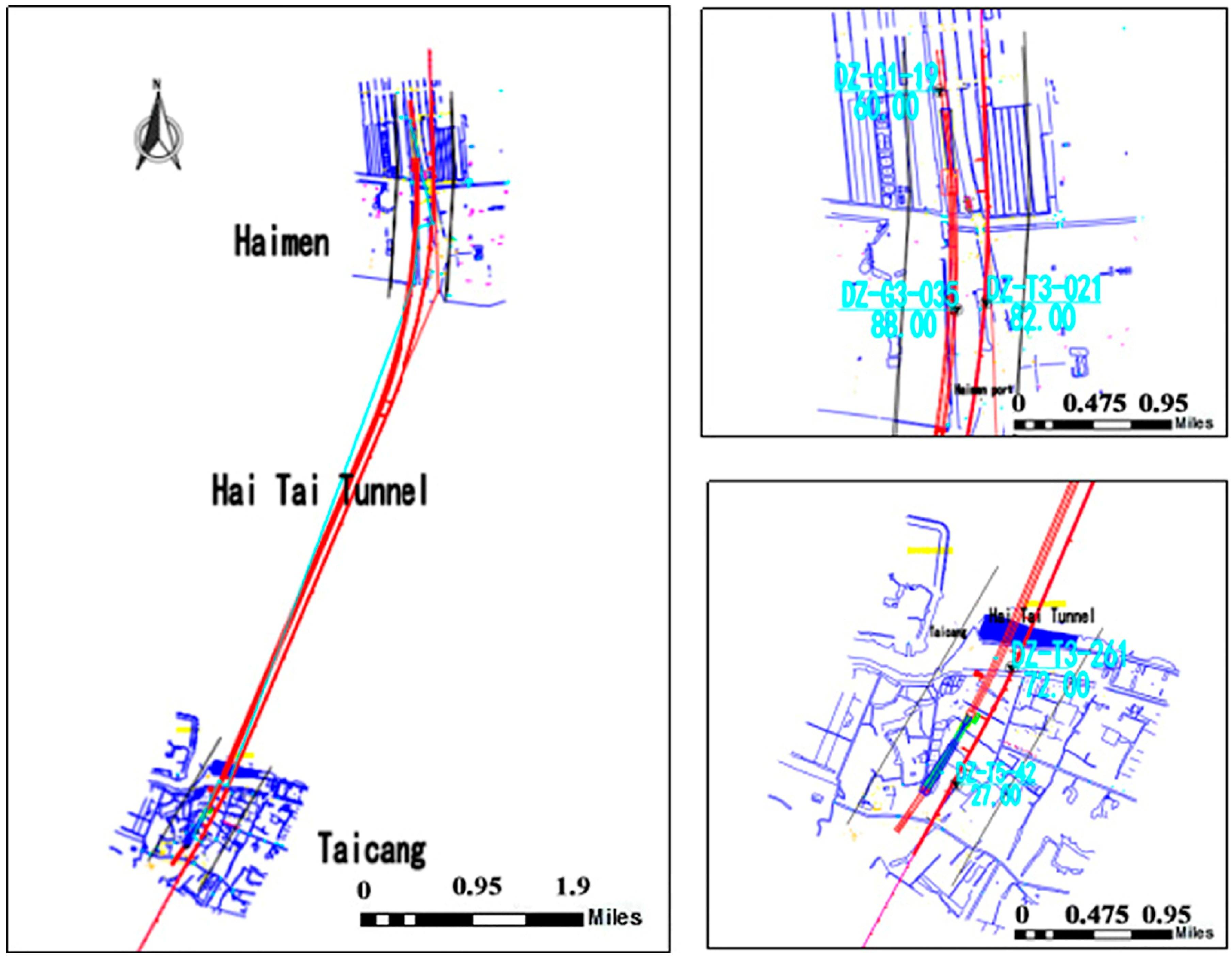
The Hai-Tai tunnel is located 8 km downstream of the Sutong Bridge. This crossing is an integral component of the ‘Yangtze River Mainline Passage Layout Planning (2019–2035)’ public rail composite river crossing, whereby the highway segment constitutes a pivotal element of the ‘Jiangsu Provincial Expressway Network Planning’, specifically the Nantong–Changshu Expressway. Furthermore, the railway component forms part of the ‘Jiangsu Provincial Intercity Railway Construction Planning for the Jiangjiang Urban Agglomeration’, including the Tongxuhu Intercity Railway River Crossing Facilities. The construction program for the Hai-Tai tunnel project adopts a three-tube tunnel design, incorporating a synchronous public rail design strategy. The Hai-Tai- Highway uses a double-tube tunnel: the starting point is connected to the proposed Tongxi Expressway (S19) and laid along the west side of the proposed Nantong New Airport, then it crosses with the Shanghai–Shaanxi (G40) and Ningqi Railway in the northwest of Haimen District, crosses the Yangtze River and terminates at the Huwu Expressway (G4221), with a length of about 58 km. The route subsequently extends towards the northwest of Haimen District and traverses the Shanghai–Shaanxi Expressway (G40) and the Ningqi Railway. Following this, it reaches the Shanghai–Wuxi Expressway section (G4221), which is located approximately 58 km downstream from the starting point. The river-crossing section of the highway utilizes a double tube tunnel, with a total length of 11.185 km, comprising a shield section of 9.315 km. The railway component traverses the Yangtze River through a single-tube tunnel, and has a total length of 11.360 km, of which the shield section is measured at 9.25 km (Figure 1).
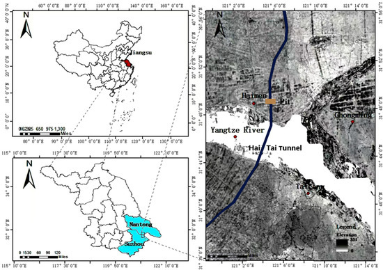
Figure 1.
Location of Hai Tai tunnel (The color-coded areas on the map are the locations of the study area).
2.2. Engineering Geological and Hydrogeological Conditions
The Hai Tai tunnel is situated within the alluvial and alluvial plain region of the Yangtze River Delta (the quaternary delta plain area), characterized by a flat and expansive topography, predominantly comprising agricultural land and village settlements. The ground elevation in this region varies between 2 and 4 m. The highest point is situated at the Yangtze River dyke, where the dyke’s flanking on either side attains an elevation of 8 m. The distance between the two points is 8.2 km and the surface of the water is 6.8 km wide, with a maximum depth of 20 m. The Haimen District is situated in the southeastern region of Jiangsu Province, with a latitude ranging from 31°46′ N to 32°09′ N and a longitude spanning from 121°04′ E to 121°32′ E. Additionally, it stands as the second-most critical region within Jiangsu Province. The terrain is relatively flat, with a network of ditches and rivers. The average elevation of the ground surface is 3–5 m. A subtle elevation gradient is observed from the northwest to the southeast, whereby the highest point reaches 5.2 m in the western region, and the lowest point is recorded at 2.5 m. In the east, Taicang is situated in the south-eastern region of Jiangsu Province, with a latitude ranging from 31°20′ to 31°45′ N and a longitude spanning from 120°58′ E to 121°20′ E. The total area is 809.93 km2, of which 143.97 km2 is occupied by the Yangtze River. The remaining 665.96 km2 constitutes the land area. Taicang is situated within the alluvial plain of the Yangtze River delta. The terrain is characterized by a flat topography, with a slight tilt from north-east to south-west. The eastern region encompasses a plain along the river, while the western area comprises a low-lying polder region.
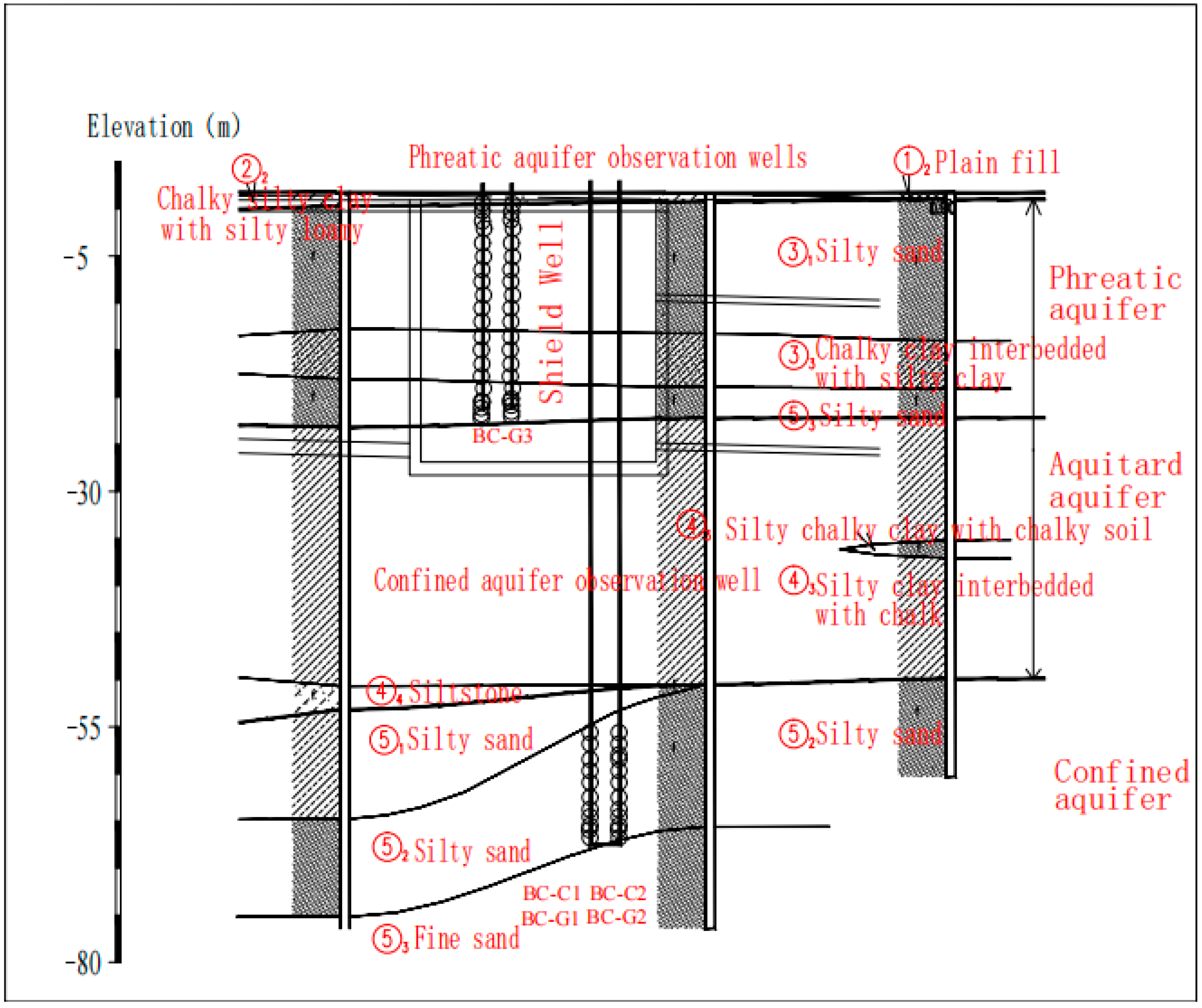
The distribution of Quaternary strata along the project corridor is notably extensive, indicating significant changes in the potential factors and characteristics controlling lithology, mainly consisting of estuarine and marine continental sediments. The main sedimentary forms observed are estuarine and marine continental interbedded sediments. The regional stratigraphic data and drilling results indicate that the lower boundary of the Holocene stratum is typically located at depths of 50–60 m, while Pleistocene strata are typically located at depths of 300–350 m. Detailed investigation and drilling data indicate that the exposed strata in the project area are mainly composed of plain fill, chalk, silty chalky clay, and interbedded silty and fine sand (Figure 2).
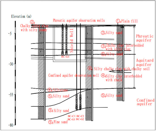
Figure 2.
Engineering geological profile of the study area.
2.3. The Hydrogeological Condition
The project is located within the Quaternary soil layer, which traverses the entire length of the project route. The hydrogeological characteristics show that groundwater storage conditions are optimal. There is phreatic water in the surface layer and confined water in the lower part. Both the water table of the phreatic water and the piezometric level of the confined water are independent and have their own characteristics. Phreatic water is mainly related to the loose soil aquifer on the surface. The thickness of the aquifer varies greatly and its distribution is discontinuous, and the seasonal variation in the water level is 1.0 to 3.0 m. In contrast, the confined water in the sand layer in the lower part of the site displays a substantial thickness of the aquifer, a continuous and optimal distribution, and is recharged by the infiltration of surface water, which is relatively abundant. This aquifer serves as the principal water source at the site, demonstrating negligible fluctuations in water levels.
As depicted in Figure 2, the phreatic aquifer consists of the following units: ① fill, ③1 silty sand, and ③2 chalky clay interbedded with silty clay. The thickness of the aquifer is 18.9 to 26.9 m. The submarine aquifer is primarily composed of powdery clay interbedded with chalk clay, with an elevation of −18.1 to −26.1 m and a burial depth of 19.9 to 27.9 m. A portion of the area is linked to the first confined water in the lower region, exhibiting slight confinement characteristics. The confined aquifer, representing the initial phase of confined water, is distributed extensively across the area, exhibiting a similar distribution range to that of the phreatic aquifer. The water-bearing medium is primarily composed of ④4 siltstone, ⑤2 silty sand, ⑤3 fine sand, and ⑤4 gravelly medium to coarse sand in the deeper strata. The thickness of the water-bearing layer within the survey area ranges from 72 to 81 m. The upper ④2 powdery clay interbedded with chalk is the confined water aquitard and forms the top plate of the confined water aquifer. The elevation of the top plate ranges from −23.8 to −50.8 m, with a depth of 25.6 to 52.6 m and a thickness of 2.2 to 25.7 m. Locally, certain sections are absent, delineated by layers of silty clay interbedded with silty sand, which maintain hydrogeological connectivity with the overlying phreatic aquifer. The lower bottom plate is a lacustrine sediments stratum (Q2l), which is locally interbedded with a fluvial facies (Q2al) stratum. The predominant lithology is characterized by hard clay, which is partially interbedded with dense, fine-grained sand. The lowest elevation of the aquifer is −130 m.
2.4. Dynamic Characteristics of Groundwater
Two phreatic and two confined long-term observation boreholes have been installed on the north bank, with observations commencing on 8 September 2021. Additionally, three long-term observation boreholes (two phreatic and one confined) have been retained at the pumping test site, with water-level observations initiated on 5 April 2022. Therefore, in total, there are seven long-term observation boreholes, four of which are phreatic and three of which are confined. The monitoring results demonstrate that the phreatic water level elevation ranges from 0.32 to 2.50 m. It is evident that the groundwater level is significantly influenced by seasonal rainfall, exhibiting a higher elevation during the rainy season. The annual variation in the water level is 2 to 3 m. The water level elevation of the first confined water layer ranges from −0.95 to 1.5 m, with an annual variation of 1 to 2 m. Furthermore, there is no discernible cyclical variation in the groundwater level, indicating that the Yangtze River’s tide level has a negligible influence on groundwater dynamics.
In order to gain insight into the relationship between the groundwater level and the water level of the Yangtze River, seven long-term observation holes were established on the north bank of the river, with observations conducted from 1 to 30 April 2022 (Figure 3). The frequency of observation was once a day, and the results of water level statistics are listed in Table 1. As illustrated in Table 1, the observed fluctuation in the Yangtze River’s water level was quantified at 2.7 m. The groundwater table exhibited a comparatively low variability. Consequently, its levels were found to be minimally influenced by the tidal fluctuations of the Yangtze River. The maximum variation recorded at the DZ-G3-068 observation well, located in close proximity to the Yangtze River, was documented as 0.11 m. The results of geological exploration indicate that the Yangtze River on the north bank was predominantly cut through strata of type ②2 (silt, silt clay) and type ③3 (silt). The tidal water levels of the Yangtze River display the most significant fluctuations within the type ②2 strata. Due to the relatively low permeability coefficient, the tidal water level of the Yangtze River does not penetrate the groundwater on either side within a short timeframe. Consequently, the fluctuations in groundwater levels on either side of the river are minimal.
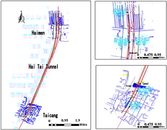
Figure 3.
Location of long-term observation holes for groundwater level.

Table 1.
Relationship between groundwater level and water level of Yangtze River (north bank).
3. Method
3.1. Mathematical Model
The three-dimensional mathematical model of groundwater flow movement can be expressed as [15]
where, Kxx, Kyy, Kzz are the components of permeability coefficient in the x, y, z direction, H is the hydraulic head, W is the flow rate per unit volume, representing the recharge and discharge of water in the study area, SS is the specific storage or specific yield of the porous medium, t is the time, H0 (x, y, z) is the initial hydraulic head of each layer in the study area, q (x, y, z, t) is the flow rate per unit area of each layer in the study area on the boundary of the second category, Γ1, Γ2 are the first and second type boundaries, respectively, and n is the inner normal on the boundary of the confined aquifer.
3.2. Optimization Model for Pit Dewatering
The mathematical model for optimizing foundation pit dewatering based on multi-objective optimization method includes three components: design variables, objective function, and constraints. The multi-objective optimization approach is employed to construct the mathematical model of pit dewatering optimization. In this model, the minimum total cost of dewatering is designated as the objective function, while other variables, such as the depth of the impervious curtain, the depth, location, number of dewatering wells, pumping rate, pumping time, and filter length and location, are taken as the design variables. At the same time these variables are taken, the optimization is carried out for the impervious curtain and the dewatering wells. The depth of the design drawdown and the maximum allowable settlement at the observation point outside the pit are taken as the constraints. The design variables are interconnected and optimally combined using numerical simulation software (FEFLOW). This software serves to analyze the interrelationships and optimal configurations of the design variables. Finally, the optimal dewatering scheme is determined according to the actual project cost. This methodology yields a more comprehensive understanding of dewatering processes for analogous pit projects.
3.2.1. Design Variable Selection
In the field of design variables, the term ‘dimension’ is often used to describe the number of variables, commonly referred to as the decision variables. Within the framework of pit dewatering, the main design variables encompass depth, location, the number of well clusters, the pumping rate, the duration of pumping, the size and location of filters, and the depth of impervious curtains. In addition, the interrelationship between the design variables is also very complex. For example, the number and pumping rate of the descending wells, in conjunction with the length and location of the filters, determine the pumping time. Additionally, the location distribution of the descending wells exerts considerable influence on the pumping rate and the number of well clusters that satisfy the design depth of the drawdown. In this paper, the optimization of the dewatering scheme for the foundation pit project of the north shore open-cut section of the Hai Tai River Crossing Highway will be conducted, with a detailed study of the connection and optimal combination of the design variables.
3.2.2. Establishment of the Objective Function
The objective function is considered as the minimum total cost of dewatering, which is related to several variables, including the depth and number of well groups, pumping rate, pumping time, length of filters, and depth of impervious curtains. Without considering other related costs, the following mathematical expression for the objective function is established 8–11.
Here, Zmin is the total cost of minimum dewatering, A is the borehole scaling cost, n is the total number of well clusters, Li is the depth of the i-th well, p is the cost recovery rate of the well body, B is the cost of well tubing, li is the length of the filter for the i-th well, C is the cost of the filter, D is the cost required to discharge a unit of water, qi is the pumping rate of the i-th well, t is the pumping time, E is the cost of impervious curtain per unit of depth, and h is depth of impervious curtain.
3.2.3. Determination of Constraint Conditions
It is not possible to assign arbitrary values to certain design variables. They must satisfy certain constraints. Furthermore, the results of pit dewatering must also satisfy the relevant constraints, as follows [16].
- (1)
- Well pumping flow constraints
It is not possible to set the pumping flow rate arbitrarily during the pumping process. The maximum pumping flow rate of a single well should be less than the actual maximum pumping flow rate of a single well. The actual maximum pumping flow rate is determined mainly based on the well capacity constraints in the large well method.
Here, qi is the pumping flow rate of the i-th well; q(i) is the actual maximum pumping flow rate of the i-th well; qmax(i) is the maximum allowable pumping volume of the i-th well; r_i is the radius of the i-th well.
- (2)
- Maximum well-depth constraints
The depth of the pumping well cannot be set arbitrarily; rather, it must be determined based on a comprehensive assessment of various technical and environmental factors. These include the length and location of the filter, as well as the structure and thickness of the aquifer. It is important to note that the optimal depth for the pumping well lies within a specific range, and attempting to set it at an extreme value is neither feasible nor advisable. Accordingly, the depth of the pumping well should be reasonably designed in accordance with the actual engineering and hydrogeological conditions, and the depth of the pumping well should not exceed the maximum depth of the pumping well.
Here, Lmax(i) is the maximum permissible depth of the i th well; Hk is the buried depth of the pit floor; h′ is the distance of the groundwater level from the pit floor after dewatering; I is the hydraulic gradient around the pit; Lx is the horizontal distance from the mid-point of the pit to the mid-point of the pumping well; H1 is the sum of the length of the filter of the pumping well and the thickness of the build-up of the sedimentary material at the bottom of the well; and H2 is the value of the well loss.
- (3)
- Water-level constraints
It is explicitly stated in the manual on pit dewatering that the groundwater level must be reduced to a minimum depth of 1 m below the bottom of the pit, which is the actual depth of the water level. This is to ensure that the design depth of the water level is not exceeded.
Here, hw is the distance of the surface phreatic water from the bottom of the pit; Swq is the phreatic water design water level drop depth; Srq is the phreatic water actual water level drop depth.
- (4)
- Subsidence constraints
It can be reasonably deduced that dewatering in the foundation pit will result in ground settlement. Should this occur to a significant extent, it could potentially endanger the safety of surrounding buildings and highways. It would therefore be advisable to arrange for settlement observation points to be established in locations of importance. Furthermore, the settlement observed at these points should not exceed the maximum allowable settlement at the aforementioned points.
Here, Sg is the settlement at the observation point, which can be calculated according to the layered sum method; Smax is the maximum allowable settlement at the observation point, which should be determined according to the actual conditions of the engineering site or the relevant norms.
3.3. The Solution of Pit Settlement Optimization Mathematical Model
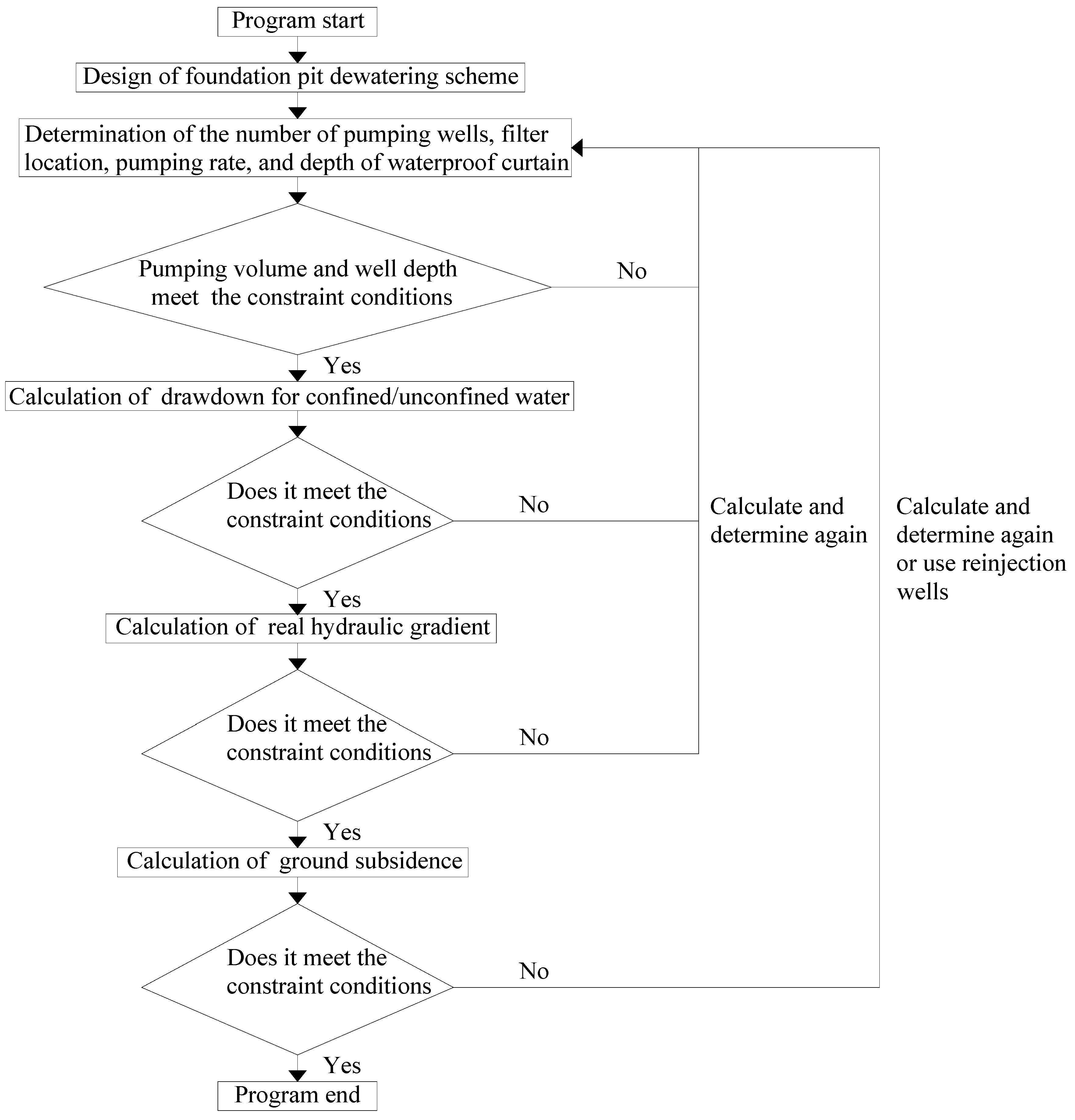
Given the numerous design variables inherent to the optimization model and the inherent interconnectivity between them, it is challenging to resolve the issue through conventional mathematical analysis techniques and optimization algorithms. Instead, a solution must be derived based on the specific conditions prevailing in the study area. This necessitates a process of continuous trial calculations and comparative analyses aimed at identifying the optimal values for the variables in question. The flow chart employed is illustrated in Figure 4. The following formula is used to calculate the vertical compression of the ground layer [17]:
where S is the vertical compression of the stratum; zg is the ground elevation; zl is the elevation of the water-containing system’s water-isolating floor or the elevation of the stratum underneath which the compression of the stratum is negligible; α is the volumetric compression coefficient of the soil; s is the depth of the water table drop caused by water pumping.
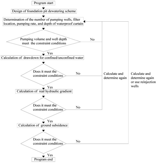
Figure 4.
Flow chart for solving optimization model of foundation pit dewatering.
4. Results
4.1. Calculation Results of Hydrogeological Parameters Based on Pumping Tests
Pumping Test of Phreatic Aquifer
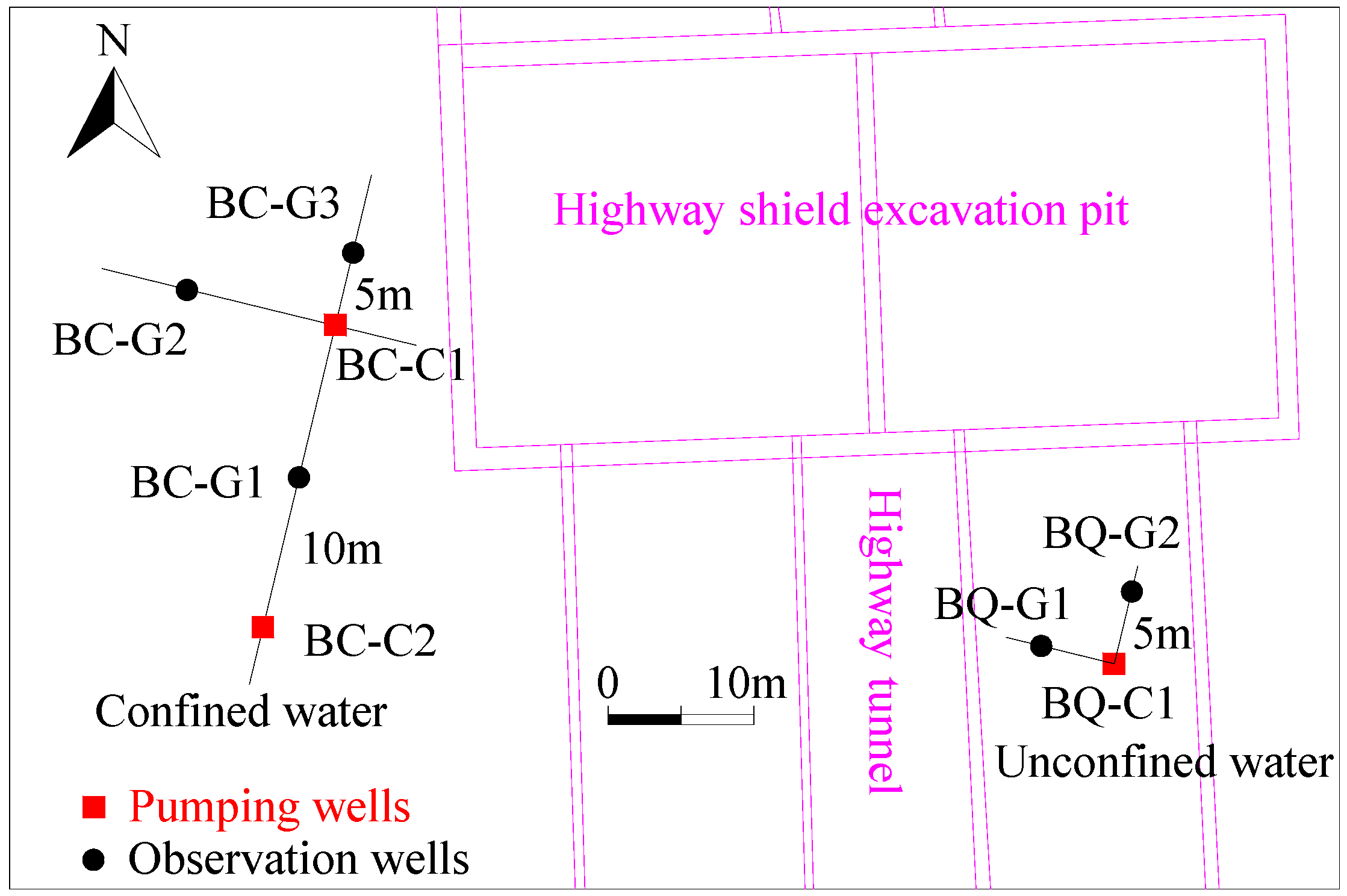
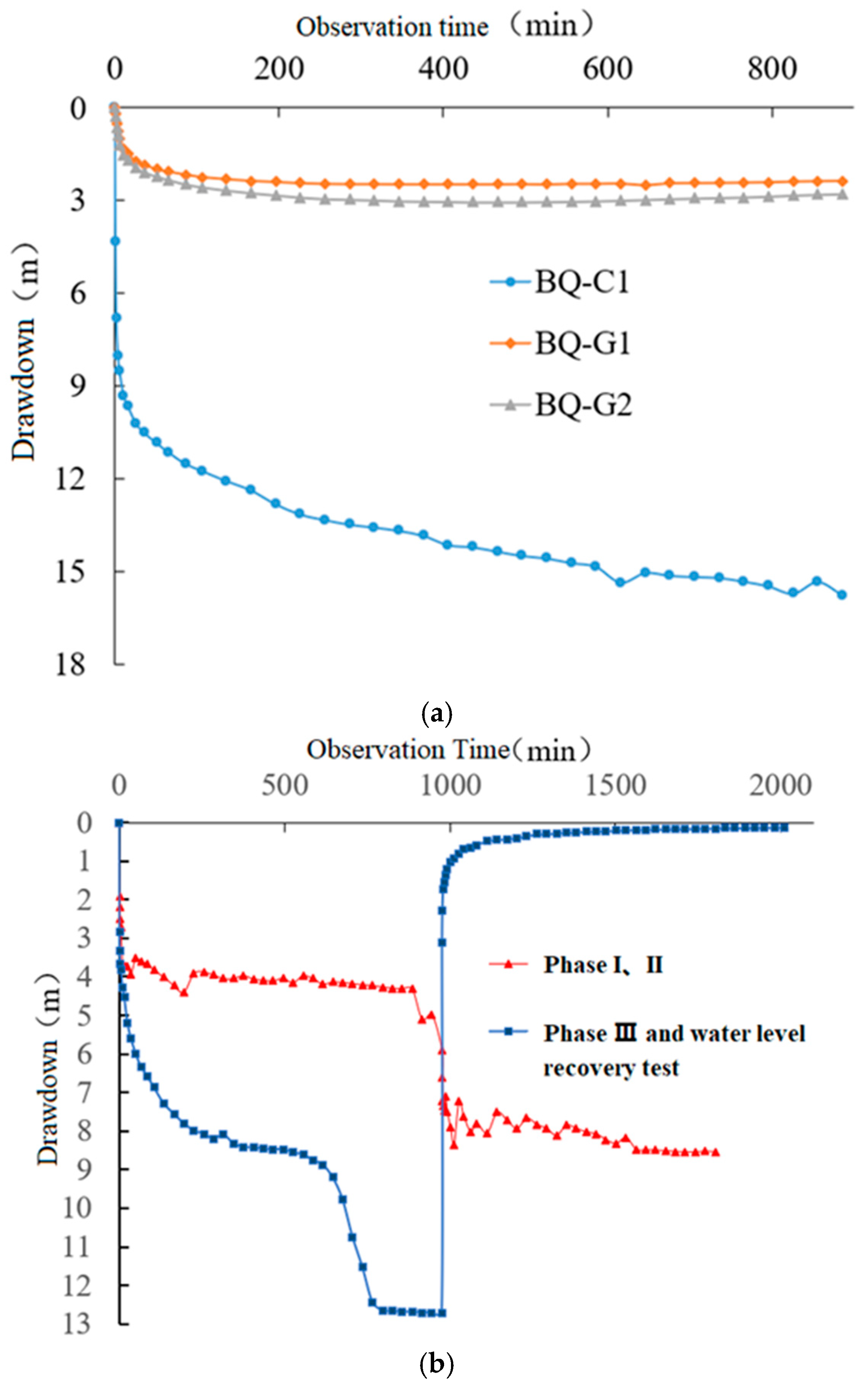
Three phreatic pumping tests were conducted in the field, and the locations of the wells in relation to the phreatic pumping tests are illustrated in Figure 5. The maximum depths of the three groundwater drops were 4.71 m, 9.14 m, and 15.33 m, with corresponding pumping rates of 274.97 m3/d, 504.76 m3/d, and 747.04 m3/d, respectively (Figure 6). The water level of the observation holes exhibited a decline between 1 and 4 m. The results of the parameter calculation are listed in Table 2. It can be observed that, as the pumping rate increases, the depth of the drawdown also increases, as does the radius of influence. The calculated permeability coefficients for each phase are essentially identical when using two observation holes, indicating that the aquifer can be considered an isotropic medium. The calculated permeability coefficients range from 1.938 to 3.523 m/d.
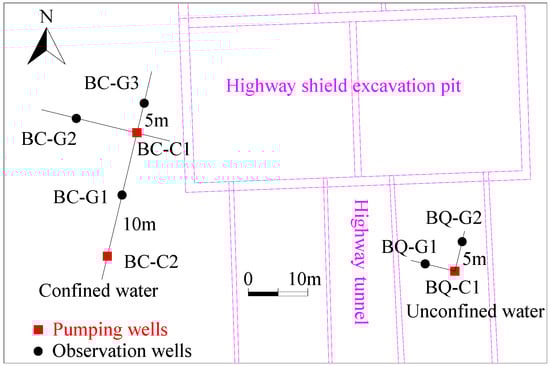
Figure 5.
Well location of pumping tests for unconfined and confined water.
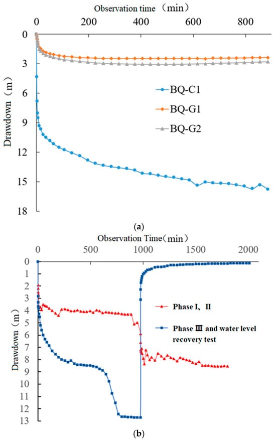
Figure 6.
Graph of pumping test data. (a) Pumping tests for phreatic aquifer. (b) Pumping tests for confined aquifer.
Table 2.
Calculated permeability coefficients based on pumping tests.
A comprehensive series of single-well pumping tests encompassing three distinct phases was executed, with the spatial arrangement of the well clusters in relation to the confined water pumping tests clearly depicted. The single-well pumping test was conducted over a period of three days, during which the maximum depth drop observed across the three phases was 3.96 m, 8.24 m, and 9.87 m, respectively. Additionally, the drawdown in the observation holes reached 0–1 m (Table 3). The results of the single-well pumping test demonstrate that (1) the single-well surge of the confined aquifer is larger, and the depth of the drawdown is smaller; (2) the aquitard has a certain degree of water-isolation performance. When the depth of the drawdown of the pumping wells is 4–10 m, the depth of the drawdown of the phreatic observation holes (BC-G3) at a distance of 5 m is less than 10 cm, and the depth of the water level in the aquitard (BRT) at a distance of 14 m is less than 2 cm, which is basically unchanged. The calculated results of the permeability coefficients are listed in Table 4, and these results account for the impact of well loss. As can be observed in Table 4, the permeability coefficients of the confined aquifer are 7.33 to 12.486 m/d.
Table 3.
Statistics of water level changes in the test holes during pumping.
Table 4.
Calculation results of hydrogeological parameters.
4.2. Identification of Model Parameters Based on Numerical Methods
In consideration of the actual topographical configuration of the phreatic pumping test site, it can be observed that the topography is relatively undulating to a lesser extent. Consequently, all of the aforementioned layers are treated as horizontal. The thickness of the phreatic aquifer is 30 m, the confined aquifer is taken as 60 m, and the aquitard is 22 m. The main pumping strata are the phreatic aquifer and the confined aquifer. Based on the radius of influence obtained by the large well method, the distance between the model boundary and the pit is 300 m, and the model boundary is set as the first boundary, and the boundary water level is the measured water level. In addition, the drainage well is not used as a boundary condition, and the size of the pumping rate is assigned directly. The bottom of the model is the water-isolated boundary. The aquifer was deemed to be homogeneous and anisotropic due to the limited lithological variation observed within the study area. A triangular mesh dissection was used, comprising 8470 nodes and 13,008 cells (Figure 7).
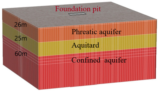
Figure 7.
Three-dimensional numerical model of pumping test site.
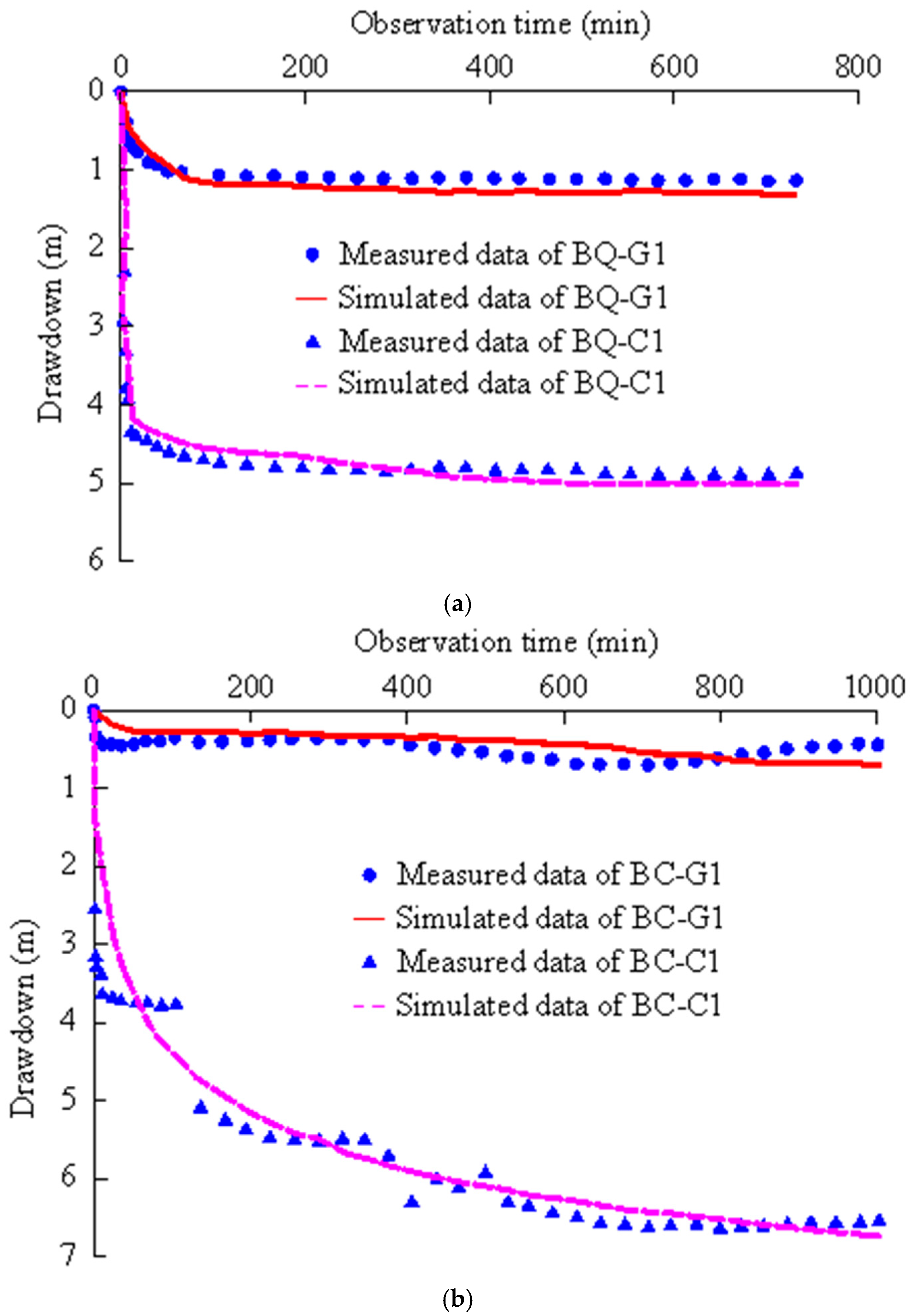
In the context of parameter inversion, the results obtained from the pumping test calculations were utilized as the initial reference values. The initial value of the groundwater permeability coefficient was 1.938–3.523 m/d, while the initial value of the permeability coefficient of confined water was 7.33–12.486 m/d. Meanwhile, referring to the difference between the observed and simulated water levels in the pumping test holes, the hydrogeological parameters in the numerical simulation are continuously adjusted, and the final hydrogeological parameters are obtained through the inversion results (Figure 8). As illustrated in Figure 8, the correlation between the measured and simulated water levels exhibits a higher precision, with an error margin of ±3.5%. This indicates that the inverted hydrogeological parameters are more reliable. Ultimately, the horizontal and vertical permeability coefficients of the phreatic aquifer were determined to be 3.0 m/d and 0.45 m/d, respectively, while the horizontal and vertical permeability coefficients of the confined aquifer were found to be 10.28 m/d and 1.25 m/d, respectively.
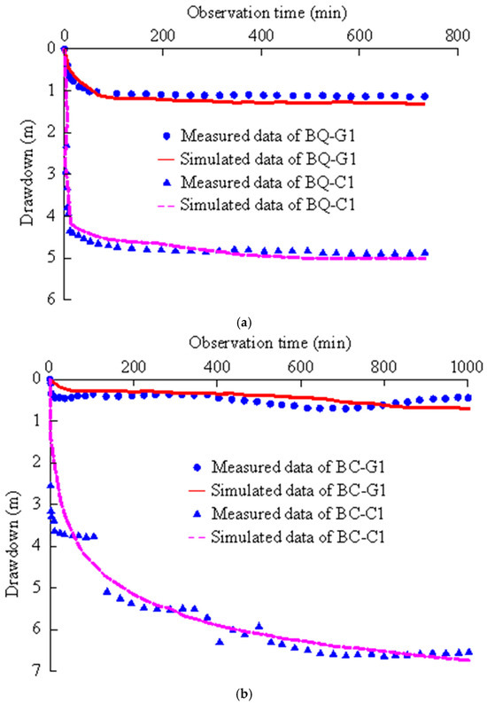
Figure 8.
Fitting diagram of the measured and simulated groundwater levels at the test site. (a) Pumping tests for phreatic aquifer. (b) Pumping tests for confined aquifer.
4.3. Optimization Study of Shield Shaft Pit Dewatering Scheme
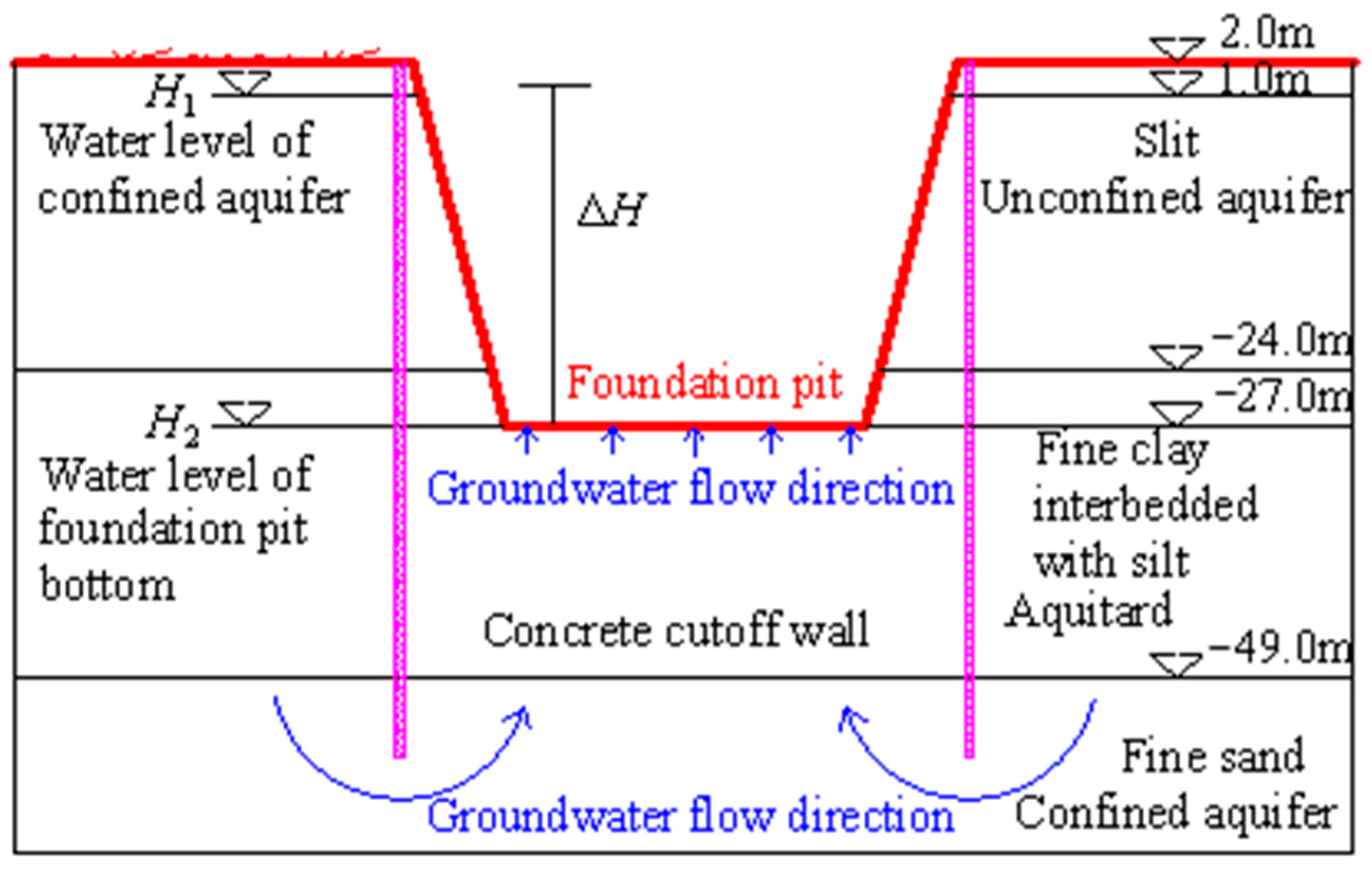
The aquifer underlying the shield pit can be categorized into three distinct strata. The upper layer is a phreatic aquifer, with a layer thickness of 26 m and water level of 2 m. The middle layer is an aquitard, comprising primarily silty clay interlayered with chalky soil, with a layer thickness of 25 m. The third layer is a confined aquifer, with a layer thickness of 60 m and a water level of 1 m. The thickness of the impervious curtains has been set at 1.2 m, with a depth of 66 m and a permeability coefficient of 1 × 10⁻⁶ m/d. The size of the shield tunnel pit is 145 m long, 56 m wide, and 29 m deep. Subsidence must be monitored for pylons in the vicinity of the study area, all adhering to a maximum allowable subsidence of 20 mm as stipulated by the design specifications.
As presented in Figure 9, a comprehensive and in-depth analysis of the pit profile was carried out. Through meticulous geotechnical investigations, including advanced geophysical prospecting techniques and high-precision borehole logging, it was clearly identified that there exists a 25-meter-thick aquitard separating the phreatic and the confined aquifer. In the context of foundation pit engineering, ensuring the safety of the construction process is of utmost importance. To this end, it is essential to thoroughly drain the phreatic water to prevent potential water—related hazards such as seepage and instability. Moreover, the designed drawdown water level of the confined aquifer is precisely set at 17 m. This specific value is determined based on a combination of hydrogeological calculations, numerical simulations, and engineering experience. Given these conditions, the primary focus of optimization should be directed towards the pumping wells within the confined aquifer. The optimization of these pumping wells is crucial for efficient dewatering and to meet the requirements of the overall engineering project. When the curtain depth reaches 66 m, a systematic and step-by-step approach is adopted. First, the quantity of well clusters is incrementally increased. This increase is based on the principle of hydraulic gradient and the need to evenly distribute the dewatering effect across the entire area of the confined aquifer. By adding more well clusters, a more uniform and efficient dewatering field can be established. Secondly, the length of the filters is gradually extended. The extension of the filter length is designed to enhance the contact area between the well and the confined aquifer, thereby improving the extraction efficiency of the confined water. This is supported by the theory of groundwater flow and the concept of well–aquifer interactions. Thirdly, the pumping rates are carefully adjusted. Different pumping rates are tested to assess their impact on the dewatering process. The adjustment of pumping rates is not only related to the efficiency of dewatering but also to the potential influence on the surrounding environment, such as ground settlement. Under the premise of not affecting the overall construction progress and safety of the project, the layout of the pumping wells is optimized. The pumping wells are arranged as close as possible to the perimeter of the pit. This is to maximize the dewatering effect near the excavation area. According to the perimeter length of the pit, the required number of pumping wells, and other relevant factors, the pumping wells are evenly distributed around the perimeter of the pit at equidistant intervals. This equidistant arrangement is based on geometric and hydraulic principles to ensure a uniform dewatering effect. Through repeated calculations, numerical simulations, and on-site monitoring, the reasonable location of the well group is finally determined, thus achieving Case 1. The optimized design of Case 1 provides a solid foundation for the subsequent optimization of and improvement in the dewatering scheme.

Figure 9.
Schematic diagram of shield tunnel foundation pit.
The optimization framework, which is firmly grounded in the dewatering Case 1, is established on the premise that all other variables remain strictly constant. This allows for the exploration of the impact of individual parameter variations. Specifically, when focusing on the filter positioning, a series of theoretical analyses and numerical simulations are carried out. By precisely adjusting the spatial location of the filters within the well system, taking into account factors such as the flow patterns of the confined aquifer and the distribution of hydraulic gradients, the design of Cases 2–3 is derived. These cases represent different scenarios of filter placement, which are crucial for understanding how filter position influences the overall dewatering efficiency.
Analogously, for the adjustment of filter length, in-depth research is conducted. The length of the filter is a key parameter affecting the well–aquifer interaction. By incrementally increasing the filter length, the surface area of contact between the well and the confined aquifer is enlarged. This change affects the rate of water extraction and the distribution of drawdown around the well. Through comprehensive numerical modeling and field-validated calculations, Cases 4–5 are formulated, which provide insights into the relationship between filter length, pumping efficiency, and water-level drawdown.
Furthermore, the investigation into the impact of single-well pumping flow is also significant. When reducing the pumping flow of a single well, the stability and uniformity of the dewatering process under low-flow conditions are analyzed. This analysis involves studying the temporal and spatial variations of the water table, the potential for non-uniform drawdown, and the long-term sustainability of the dewatering system. Based on these considerations, Cases 6–7 are developed. Conversely, when increasing the pumping flow of a single well, both the impact on the dewatering speed and the potential effects on the surrounding environment, such as ground settlement and changes in the stress field of the soil, are thoroughly examined. This leads to the generation of Cases 8–9.
The simulation results, obtained through a combination of advanced numerical models and real-time field monitoring data, show that the drawdown rate of the pressurized pumping wells remains basically stable within 0.5 days. After this initial period, it increases slowly with the increase in dewatering time. In more detail, if other conditions remain unchanged, increasing the pumping rate of a single well does not shorten the time required to reach the design drawdown rate. Instead, it may cause the drawdown to exceed the design drawdown rate of the pressurized water. This over-drawdown situation can lead to a series of problems. For example, it increases the actual hydraulic gradient at the bottom of the pressurized pumping wells. Once this hydraulic gradient exceeds the critical hydraulic gradient of the flowing soil, it will seriously threaten the normal operation of the foundation pit, potentially causing soil liquefaction, instability, and other geotechnical hazards. Moreover, it will also increase the total cost of the foundation pit dewatering project due to the need for additional measures to address the adverse effects.
In summary, through a comprehensive evaluation of all cases, considering factors such as dewatering efficiency, cost-effectiveness, and environmental impact, Case 8 is identified as the optimal scheme for the 66-metre curtain depth case (as clearly presented in Table 5). Similarly, when the curtain depth is 61 m and 56 m, respectively, Case 9 and Case 10 are determined to be the optimal choices (Table 5). These optimal cases provide valuable references for practical foundation pit dewatering projects, guiding engineers to make more informed decisions and design more efficient and safe dewatering systems.
Table 5.
Summary of dewatering schemes for the 66 m impervious curtain.
The computational results exhibit a remarkable similarity to those obtained during the optimization process of the phreatic drawdown within the phreatic water pit. To begin with, a comprehensive set of computational methods was employed, including finite-element numerical simulations and analytical solutions based on established hydrogeological theories. These methods were rigorously validated against field-measured data to ensure their accuracy and reliability.
Typically, the drawdown in the confined pumping well demonstrates stable behavior within a time span of 0.5 days. This stability is attributed to the initial equilibrium state of the groundwater system and the relatively slow response of the aquifer to the pumping action. As the dewatering duration extends, the drawdown gradually increases. This increase can be explained by the continuous extraction of water from the confined aquifer, which leads to a progressive decline in the hydraulic head.
When considering the impact of individual well pumping rate, an in-depth analysis was carried out under the assumption that all other factors remain constant. It was found that increasing the pumping rate of an individual well does not contribute to shortening the time required to reach the design drawdown level. On the contrary, such an increase may cause the drawdown to exceed the design drawdown rate for confined water. This over-drawdown situation is mainly due to the non-linear relationship between the pumping rate and aquifer response. As the pumping rate increases, the aquifer’s ability to transmit water may become saturated, resulting in an excessive decline in the water level.
The results of the calculations clearly indicate that, for a curtain depth of 66 m, the optimal water reduction scheme is Case 3 (as presented in Table 5). This determination is based on a multi-criteria evaluation, taking into account factors such as dewatering efficiency, cost-effectiveness, and the impact on the surrounding environment. Similarly, through a similar process of analysis and evaluation, the optimal schemes for curtain depths of 61 m and 56 m can be derived (Table 6).
Table 6.
Summary of water descent scenarios for different curtain depths in the pit.
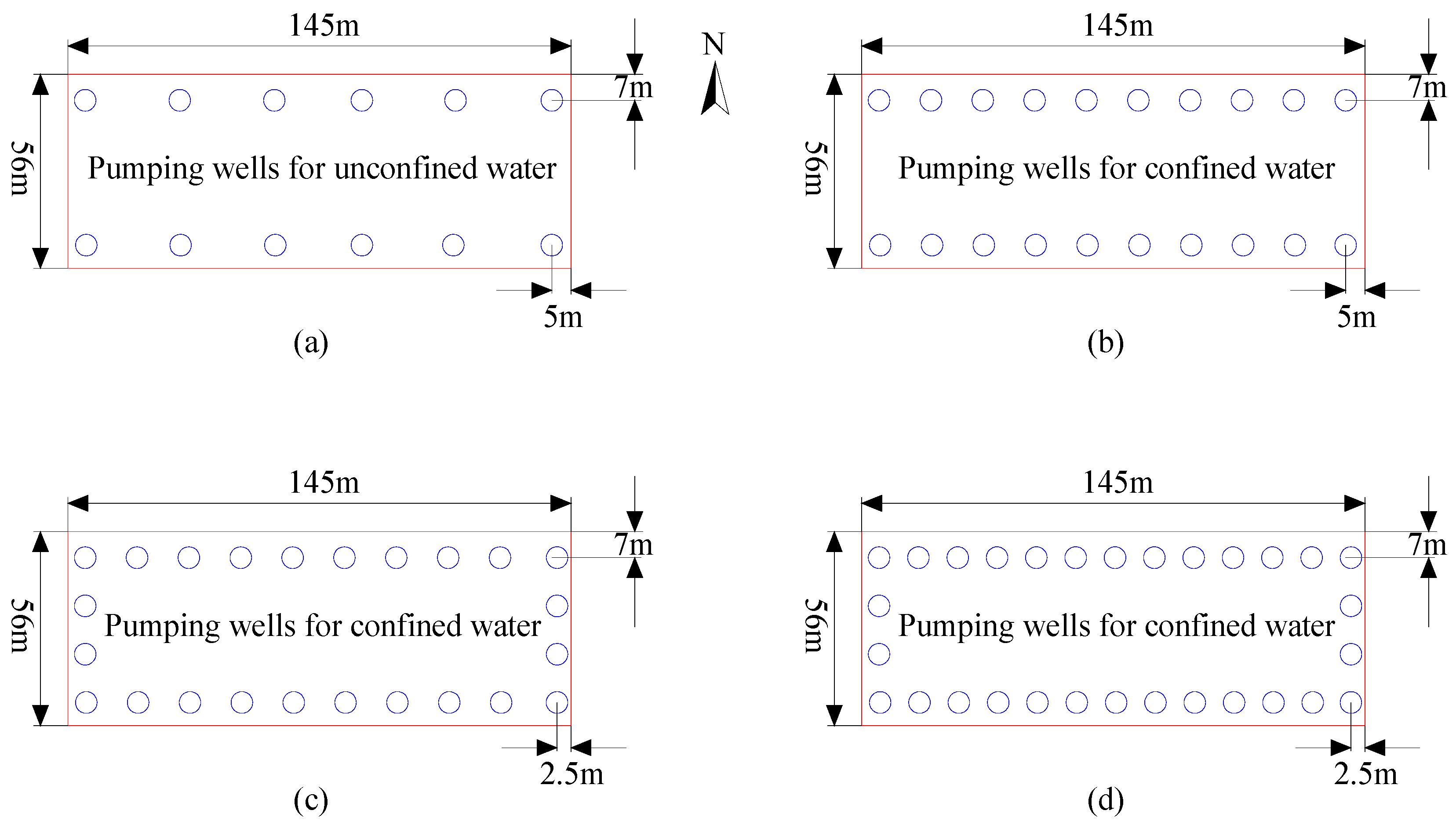
In addition, the optimal locations for the phreatic and confined water pumping well clusters are graphically illustrated in Figure 10. These optimal locations were determined through a combination of numerical simulations and field-based considerations. The simulations took into account factors such as the spatial distribution of the aquifers, the flow patterns of groundwater, and the geometric constraints of the foundation pit. The field-based considerations included factors such as the accessibility of the well locations, the impact on adjacent structures, and the ease of construction and maintenance.
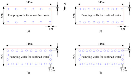
Figure 10.
Layout of pumping wells for shield tunnel foundation pit. (a) Location map of 12 unconfined pumping Wells (b) Location map of 20 confined pumping Wells (c) Location map of 24 confined pumping Wells (d) Location map of 30 confined pumping Wells.
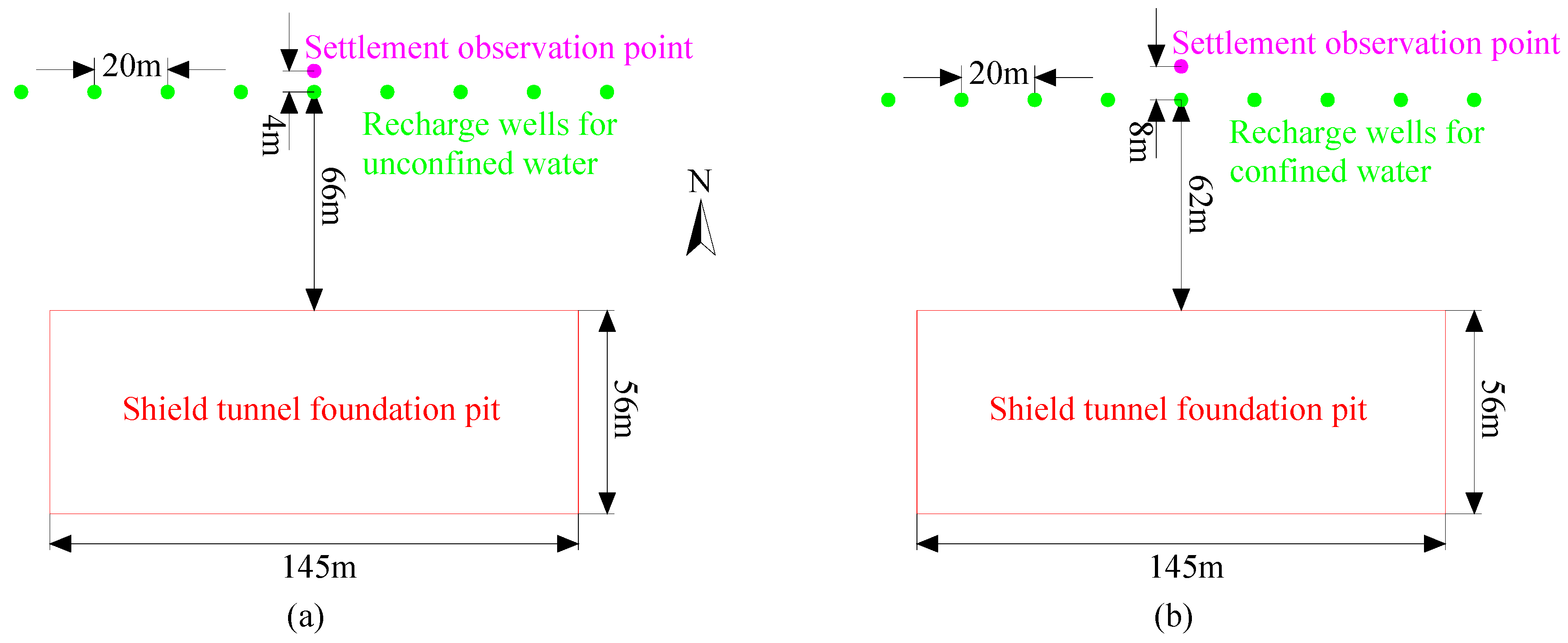
Correspondingly, the locations of the phreatic and confined water recharge well clusters are shown in Figure 11. The design of the recharge well locations is crucial for maintaining the balance of the groundwater system and minimizing the potential negative impacts of dewatering on the surrounding environment. The recharge well locations were selected to ensure efficient recharge of the aquifers and to mitigate the effects of drawdown on nearby water bodies and ecosystems.
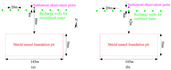
Figure 11.
Layout of recharge wells for shield tunnel foundation pit. (a) Location map of unconfined recharge Wells (b) Location map of confined recharge Wells.
5. Conclusions
This study successfully developed a mathematical model for optimizing foundation pit dewatering using multi-objective optimization methods, with the core objective of minimizing total dewatering costs. Decision variables included well group depth, lateral spacing, well number, pumping rate, operation duration, filter length, filter placement, and impervious curtain depth. The mathematical model for optimizing foundation pit dewatering using multi-objective optimization methods effectively balanced cost reduction (number of wells and pumping time savings compared to conventional designs) with environmental constraints, ensuring compliance with engineering and safety standards. Through comparison, reasonable dewatering schemes that decision variables are significantly lower included lateral spacing (7.5–27.5 m), well number (32–60), pumping rate (296.1–688.21 m3/d), operation duration (6.4–7 days), filter length (4–13.5 m), filter placement (mid-lower aquifer), and impervious curtain depth (56–66 m) for the depth of the impervious curtain in the 66 m, 61 m, and 56 m shield tunnels were determined. The results indicate that the settlement at a distance of 70 m from the pit is less than 20 mm, and the settlement at the tower at a distance of 200 m is even smaller. This discovery complies with the design specifications and ensures that there are no adverse effects. In addition, the minimum distance between the residence and the pit is about 800 m, which exceeds the impact range of foundation pit subsidence. Therefore, the impact of the foundation pit settlement on the environment and residents’ lives can be ignored. The optimization scheme has several advantages, including reducing the dewatering time, minimizing the impact of excavation dewatering on the surrounding environment, and lowering the overall dewatering cost.
Therefore, for similar dewatering projects of deep foundation pit, the multi-objective cost control method proposed in this study can be widely used as it not only saves engineering costs and construction time but can also ensure the safe construction of the project to a certain extent.
Author Contributions
Conceptualization, Z.D.; methodology, Z.D. and M.X.; validation, M.X., C.C. and Y.H.; formal analysis, Z.D. and M.X.; resources, Z.D. and Y.H.; data curation, M.X., X.H., C.C. and Y.H.; writing—original draft preparation, Z.D.; writing—review and editing, M.X. and X.H.; supervision, Z.D., C.C. and Y.H.; project administration, C.C. and Y.H. All authors have read and agreed to the published version of the manuscript.
Funding
This research was funded by the National Natural Science Foundation of China Joint Fund Project, grant number U2240217.
Data Availability Statement
Data are contained within the article.
Acknowledgments
The authors would like to acknowledge the financial support from the National Natural Science Foundation of China Joint Fund Project. The authors would also like to thank the School of Earth Sciences and Engineering at Hohai University for partial support of the graduate student on this project, support of Jiangsu Rail Transit Industry Development Collaborative Innovation Base Open Fund (GCXC2307), and support of Science and Technology Innovation Team Funding at Nanjing Vocational Institute of Railway Technology.
Conflicts of Interest
Author Zhigao Dong was employed by the company Nanjing Vocational Institute of Railway technology. Author Chunyang Chai was employed by the company China Railway Reyuan Engineering Group Co., Ltd. Author Xiushi Huo was employed by the company China Water Huaihe Planning, Design and Research Co., Ltd. The remaining authors declare that the research was conducted in the absence of any commercial or financial relationships that could be construed as potential conflicts of interest.
References
- Cao, Y.; Zhang, R.; Zhang, D.; Zhou, C. Urban Agglomerations in China: Characteristics and Influencing Factors of Population Agglomeration. Chin. Geogr. Sci. 2023, 33, 719–735. [Google Scholar] [CrossRef]
- Wang, J.; Deng, Y.; Wang, X.; Liu, X.; Zhou, N. Numerical evaluation of a 70-m deep hydropower station foundation pit dewatering. Environ. Earth Sci. 2022, 81, 364. [Google Scholar] [CrossRef]
- Zeng, C.F.; Xue, X.L.; Li, M.K. Use of cross wall to restrict enclosure movement during dewatering inside a metro pit before soil excavation. Tunn. Undergr. Space Technol. Inc. Trenchless Technol. Res. 2021, 112, 103909. [Google Scholar] [CrossRef]
- Cao, C.; Shi, C.; Liu, L.; Liu, J. Evaluation of the effectiveness of an alternative to control groundwater inflow during a deep excavation into confined aquifers. Environ. Earth Sci. 2020, 79, 502. [Google Scholar] [CrossRef]
- Wang, X.W.; Yang, T.L.; Xu, Y.S.; Shen, S.L. Evaluation of optimized depth of waterproof curtain to mitigate negative impacts during dewatering. J. Hydrol. 2019, 577, 123969. [Google Scholar] [CrossRef]
- Huang, Y.; Bao, Y.; Wang, Y. Analysis of geoenvironmental hazards in urban underground space development in Shanghai. Nat. Hazards 2015, 75, 2067–2079. [Google Scholar] [CrossRef]
- Yu, D.; Lu, J.-P.; Tang, Y.-Q. Optimal Design of Well Spacing in Foundation Pit Multi-well Dewatering Based on Objective Function. J. Shenyang Jianzhu Univ. (Nat. Sci.) 2013, 29, 649–654. [Google Scholar]
- Xu, Y. Optimal Precipitation Analysis of Well Group Based on Objective Function Method and Finite Element Method; Northeastern University: Boston, MA, USA, 2013. [Google Scholar]
- Chen, Z.; Huang, J.; Zhan, H.; Wang, J.; Dou, Z.; Zhang, C.; Chen, C.; Fu, Y. Optimization schemes for deep foundation pit dewatering under complicated hydrogeological conditions using MODFLOW-USG. Eng. Geol. 2022, 303, 106653. [Google Scholar] [CrossRef]
- Liu, L.; Lei, M.; Cao, C.; Shi, C. Dewatering Characteristics and Inflow Prediction of Deep Foundation Pits with Partial Penetrating Curtains in Sand and Gravel Strata. Water 2019, 11, 2182. [Google Scholar] [CrossRef]
- You, Y.; Yan, C.; Xu, B.; Liu, S.; Che, C. Optimization of dewatering schemes for a deep foundation pit near the Yangtze River, China. J. Rock Mech. Geotech. Eng. 2018, 10, 555–566. [Google Scholar] [CrossRef]
- Wang, J.; Wu, Y.; Liu, X.; Yang, T.; Wang, H.; Zhu, Y. Areal subsidence under pumping well–curtain interaction in subway foundation pit dewatering: Conceptual model and numerical simulations. Environ. Earth Sci. 2016, 75, 198. [Google Scholar] [CrossRef]
- Zhou, N.; Vermeer, P.A.; Lou, R.; Tang, Y.; Jiang, S. Numerical simulation of deep foundation pit dewatering and optimization of controlling land subsidence. Eng. Geol. 2010, 114, 251–260. [Google Scholar] [CrossRef]
- Alhama, I.; Carrasco, S.N.; Jiménez-Valera, J.A.; Freitas, T.M.; García Guerrero, J.M. A general solution for groundwater flow around deep excavations based on non–dimensionalization techniques. Eng. Geol. 2025, 347, 107938. [Google Scholar] [CrossRef]
- Bear, J. Hydraulics of Groundwater; McGraw-Hill: New York, NY, USA, 2012. [Google Scholar]
- Beale, G.; Read, J. Guidelines for Evaluating Water in Pit Slope Stability; CSIRO Publishing: Clayton, Australia, 2014. [Google Scholar]
- Peng, B.; Feng, R.; Wu, L.; Wei, K.; Wang, P. Settlement Calculation Method for Peat Soil Foundations. Int. J. Geomech. 2023, 23, 04023094. [Google Scholar] [CrossRef]


Disclaimer/Publisher’s Note: The statements, opinions and data contained in all publications are solely those of the individual author(s) and contributor(s) and not of MDPI and/or the editor(s). MDPI and/or the editor(s) disclaim responsibility for any injury to people or property resulting from any ideas, methods, instructions or products referred to in the content. |
© 2025 by the authors. Licensee MDPI, Basel, Switzerland. This article is an open access article distributed under the terms and conditions of the Creative Commons Attribution (CC BY) license (https://creativecommons.org/licenses/by/4.0/).