


Intercomparison of Runoff and River Discharge Reanalysis Datasets at the Upper Jinsha River, an Alpine River on the Eastern Edge of the Tibetan Plateau


Abstract
1. Introduction
2. Materials and Methods
2.1. Reanalysis Datasets
2.2. River Discharge Observations
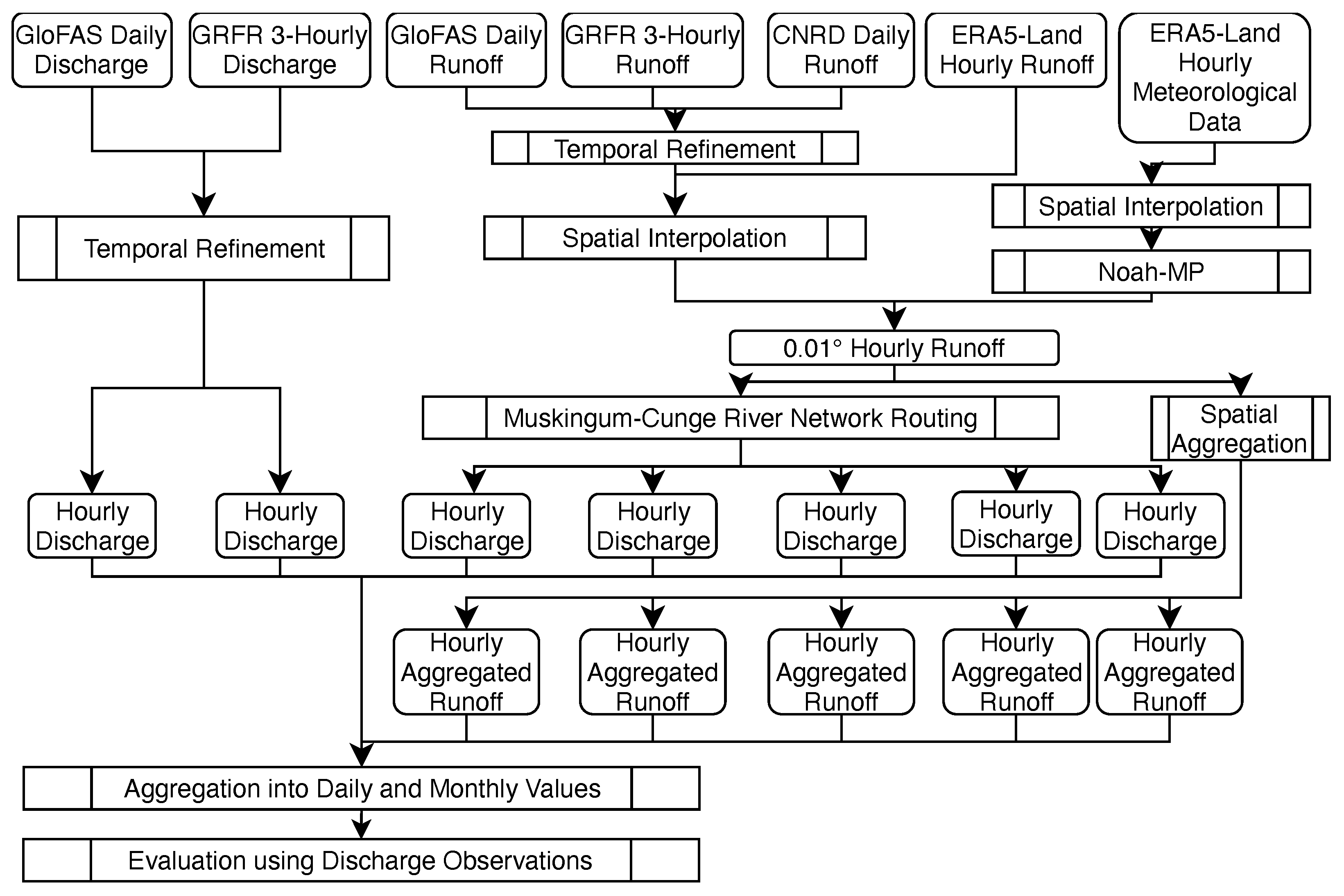
2.3. Evaluation Methods
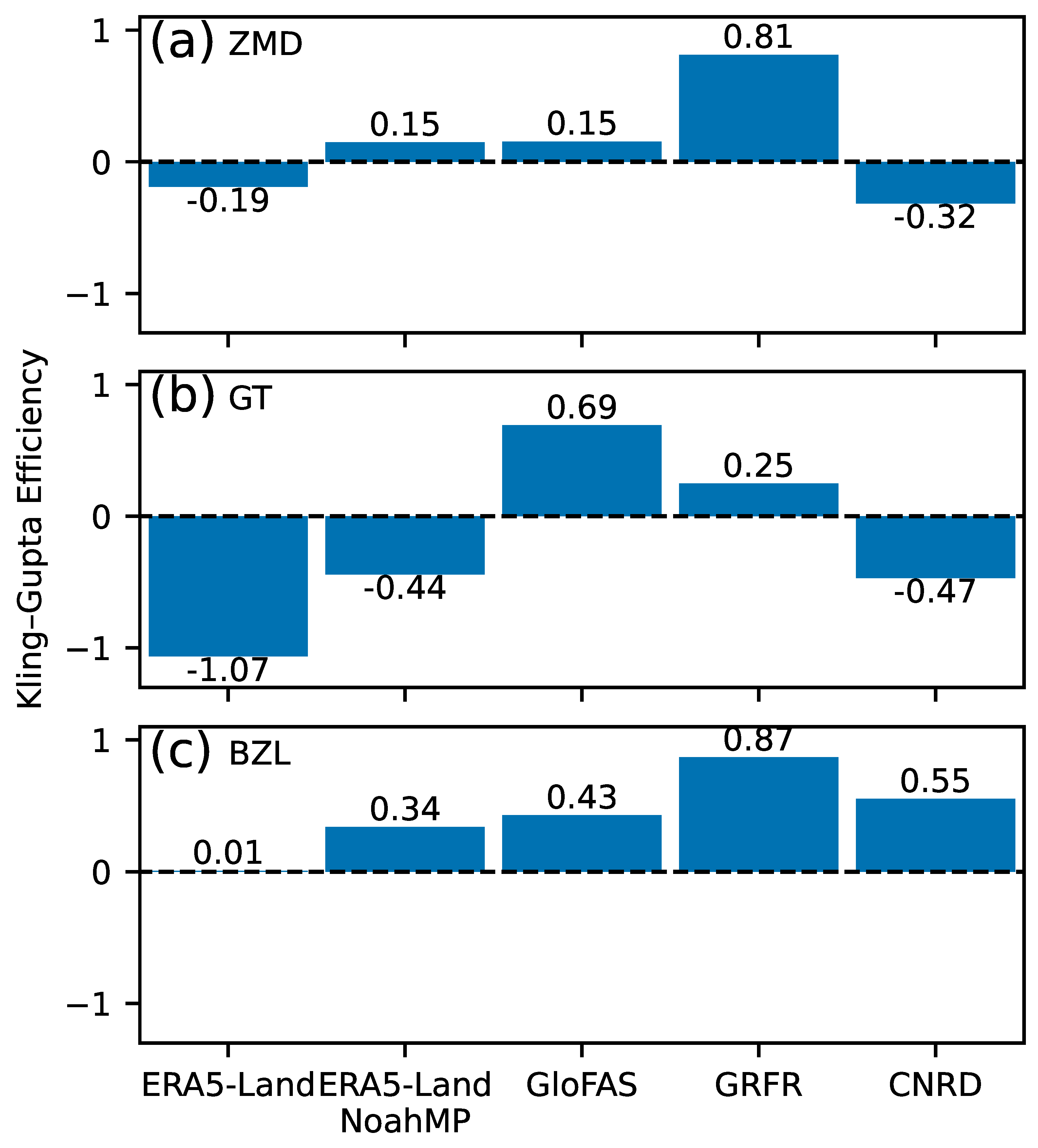
2.4. Evaluation Metrics
3. Results and Discussion
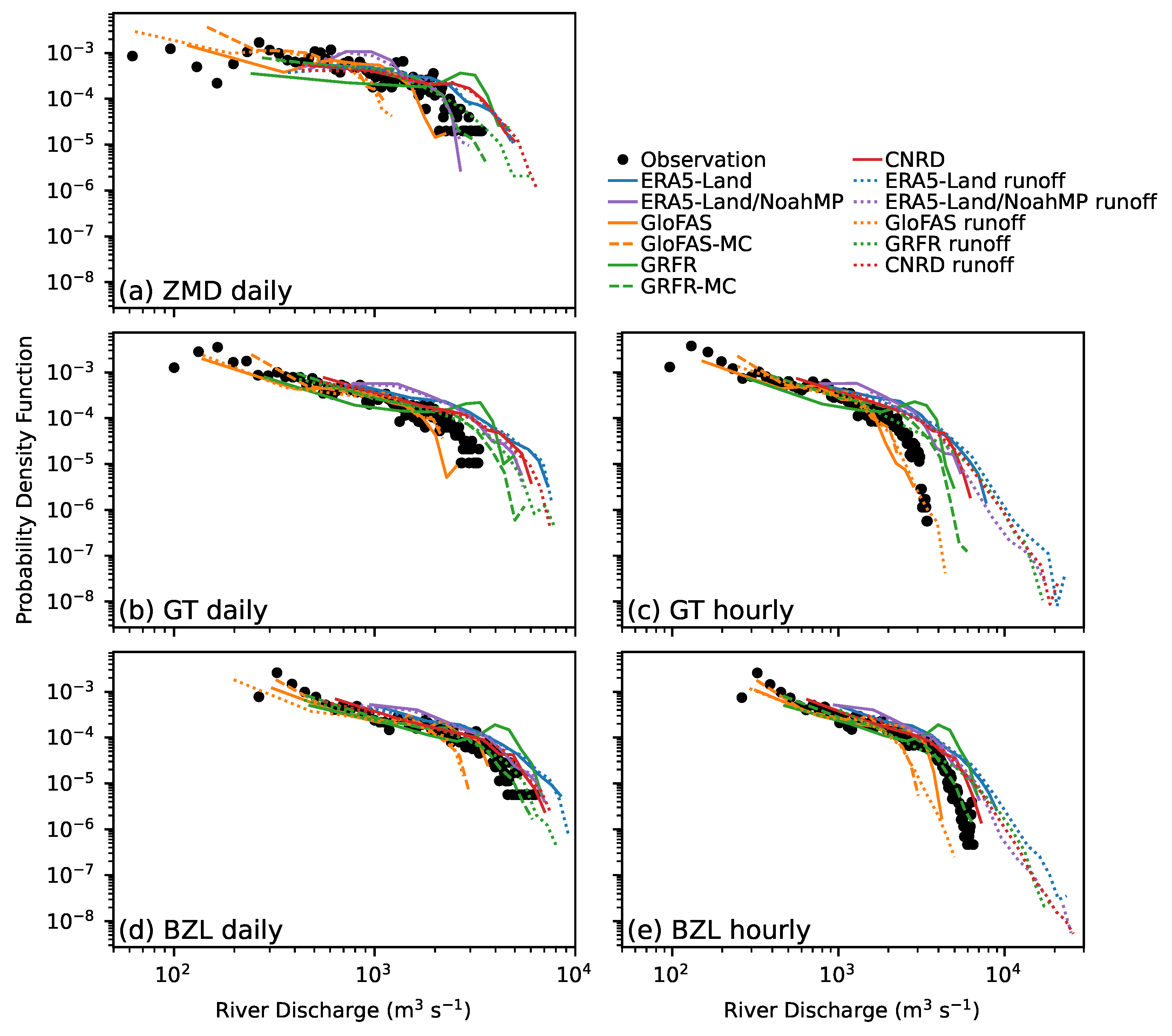
3.1. Runoff
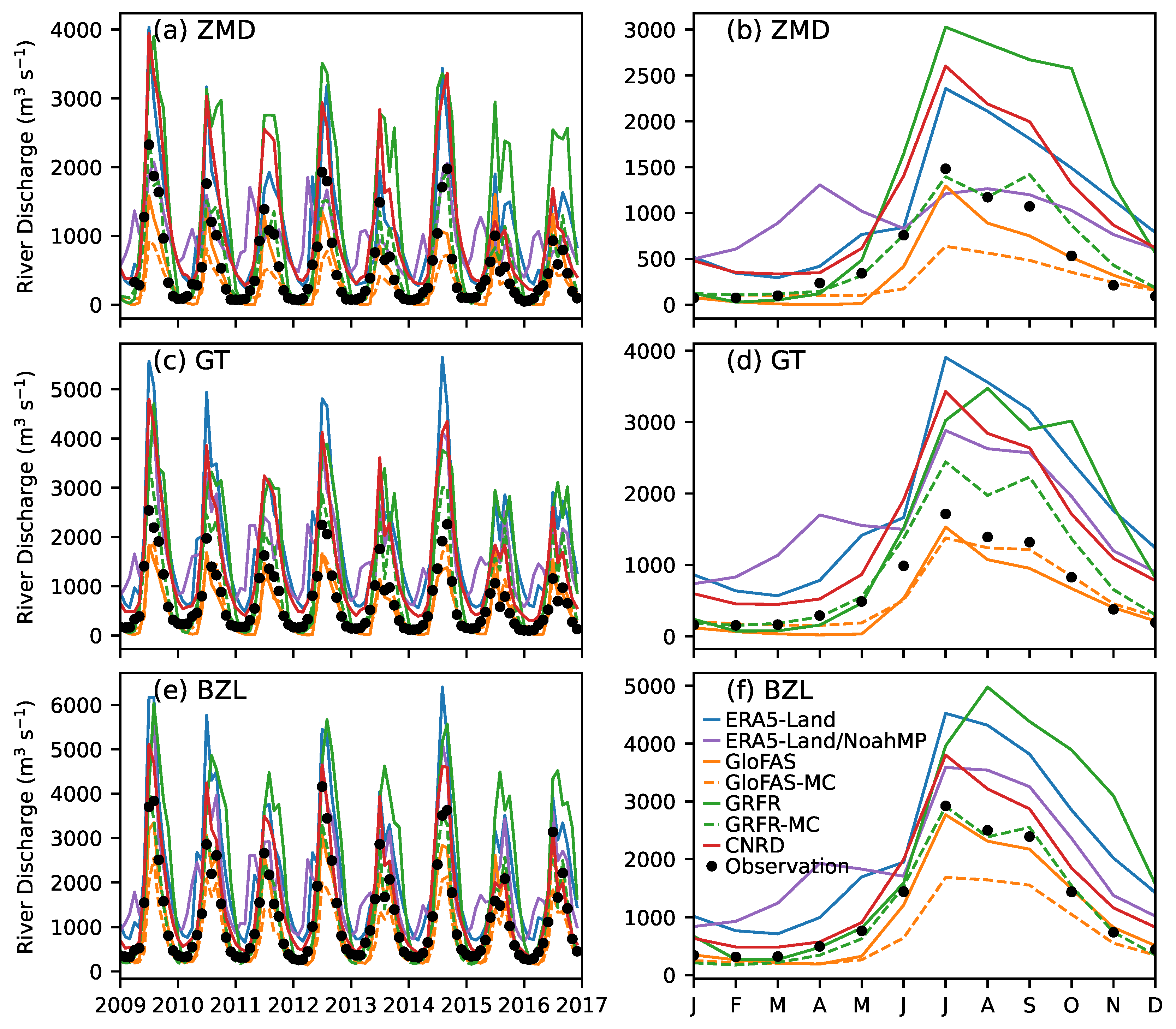
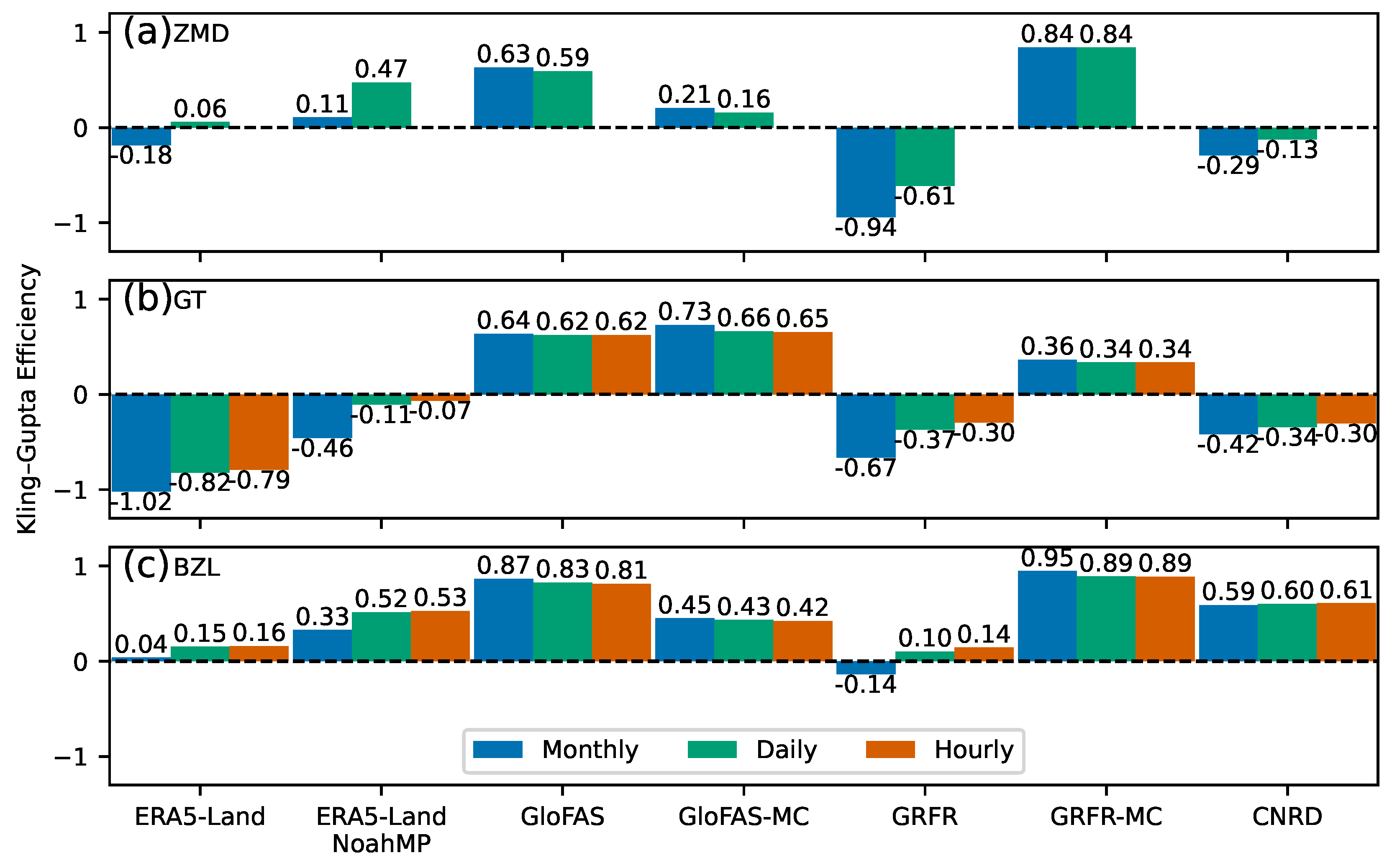
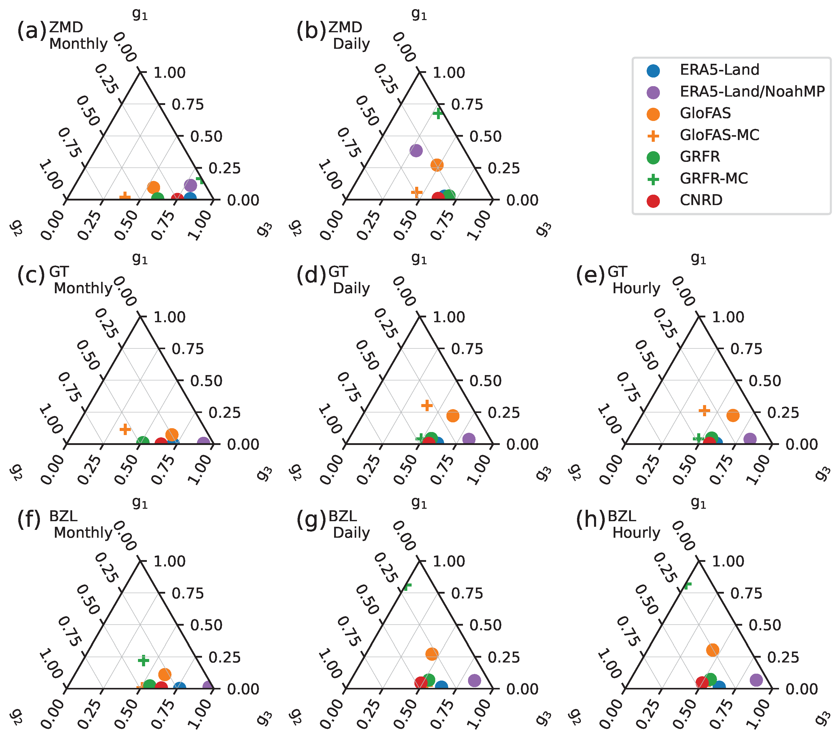
3.2. Streamflow
4. Conclusions
- Among ERA5-Land, GloFAS, GRFR, and CNRD, GloFAS performs the best in river discharge estimation. The superior performance is attributed to the extensive calibration of model parameters rather than the quality of meteorological forcing. The other datasets, driven by similar meteorological forcing but using uncalibrated models—including ERA5-Land and a high-resolution simulation conducted in this study—did not perform on a par with GloFAS.
- Despite its high skill in river discharge estimation, GloFAS’s runoff estimation is subpar. This discrepancy is attributable to the coarse resolution of GloFAS’s routing grid. A 0.1° grid cell resolution is insufficient to accurately delineate the catchment area in the study region. Since river discharge is calculated by multiplying runoff by the catchment area, errors in catchment area estimation propagate to runoff estimates during the calibration of river discharge.
- GRFR demonstrates the best performance in runoff estimation at two out of the three stations examined. The high performance of GRFR runoff is attributed to its runoff characteristics-based calibration method. However, this machine learning-based method is more sensitive to the training dataset used than the traditional method employed by GloFAS. At Gangtuo, the station with steep terrain where observations are not included in the training dataset, GRFR’s performance is subpar.
- GRFR’s river discharge estimation is unexpectedly poor. GRFR substantially overestimates river discharge, a finding consistent with previous studies. Our study confirms that the overestimation is due to inadequate settings in river routing. By rerouting the discharge using GRFR runoff and the Muskingum–Cunge routing method, we closely reproduce the observed discharge patterns, achieving the best skill among all the examined datasets.
Author Contributions
Funding
Data Availability Statement
Acknowledgments
Conflicts of Interest
References
- Hersbach, H.; Bell, B.; Berrisford, P.; Hirahara, S.; Horányi, A.; Muñoz-Sabater, J.; Nicolas, J.; Peubey, C.; Radu, R.; Schepers, D.; et al. The ERA5 global reanalysis. Q. J. R. Meteorol. Soc. 2020, 146, 1999–2049. [Google Scholar] [CrossRef]
- Muñoz-Sabater, J.; Dutra, E.; Agustí-Panareda, A.; Albergel, C.; Arduini, G.; Balsamo, G.; Boussetta, S.; Choulga, M.; Harrigan, S.; Hersbach, H.; et al. ERA5-Land: A state-of-the-art global reanalysis dataset for land applications. Earth Syst. Sci. Data 2021, 13, 4349–4383. [Google Scholar] [CrossRef]
- Alfieri, L.; Lorini, V.; Hirpa, F.A.; Harrigan, S.; Zsoter, E.; Prudhomme, C.; Salamon, P. A global streamflow reanalysis for 1980–2018. J. Hydrol. X 2020, 6, 100049. [Google Scholar] [CrossRef]
- Harrigan, S.; Zsoter, E.; Alfieri, L.; Prudhomme, C.; Salamon, P.; Wetterhall, F.; Barnard, C.; Cloke, H.; Pappenberger, F. GloFAS-ERA5 operational global river discharge reanalysis 1979–present. Earth Syst. Sci. Data 2020, 12, 2043–2060. [Google Scholar] [CrossRef]
- Yang, Y.; Pan, M.; Lin, P.; Beck, H.E.; Zeng, Z.; Yamazaki, D.; David, C.H.; Lu, H.; Yang, K.; Hong, Y.; et al. Global reach-level 3-hourly river flood reanalysis (1980–2019). Bull. Am. Meteorol. Soc. 2021, 102, E2086–E2105. [Google Scholar] [CrossRef]
- Lin, P.; Pan, M.; Beck, H.E.; Yang, Y.; Yamazaki, D.; Frasson, R.; David, C.H.; Durand, M.; Pavelsky, T.M.; Allen, G.H.; et al. Global reconstruction of naturalized river flows at 2.94 million reaches. Water Resour. Res. 2019, 55, 6499–6516. [Google Scholar] [CrossRef]
- Cosgrove, B.; Gochis, D.; Flowers, T.; Dugger, A.; Ogden, F.; Graziano, T.; Clark, E.; Cabell, R.; Casiday, N.; Cui, Z.; et al. NOAA’s National Water Model: Advancing operational hydrology through continental-scale modeling. J. Am. Water Resour. Assoc. 2024, 60, 247–272. [Google Scholar] [CrossRef]
- Najafi, H.; Shrestha, P.K.; Rakovec, O.; Apel, H.; Vorogushyn, S.; Kumar, R.; Thober, S.; Merz, B.; Samaniego, L. High-resolution impact-based early warning system for riverine flooding. Nat. Commun. 2024, 15, 3726. [Google Scholar] [CrossRef]
- Gou, J.; Miao, C.; Samaniego, L.; Xiao, M.; Wu, J.; Guo, X. CNRD v1.0: A high-quality natural runoff dataset for hydrological and climate studies in china. Bull. Am. Meteorol. Soc. 2021, 102, E929–E947. [Google Scholar] [CrossRef]
- Miao, C.; Gou, J.; Fu, B.; Tang, Q.; Duan, Q.; Chen, Z.; Lei, H.; Chen, J.; Guo, J.; Borthwick, A.G.L.; et al. High-quality reconstruction of China’s natural streamflow. Sci. Bull. 2022, 67, 547–556. [Google Scholar] [CrossRef]
- Feng, D.; Gleason, C.J.; Lin, P.; Yang, X.; Pan, M.; Ishitsuka, Y. Recent changes to Arctic river discharge. Nat. Commun. 2021, 12, 6917. [Google Scholar] [CrossRef] [PubMed]
- Collins, E.L.; David, C.H.; Riggs, R.; Allen, G.H.; Pavelsky, T.M.; Lin, P.; Pan, M.; Yamazaki, D.; Meentemeyer, R.K.; Sanchez, G.M. Global patterns in river water storage dependent on residence time. Nat. Geosci. 2024, 17, 433–439. [Google Scholar] [CrossRef]
- Liu, M.; Raymond, P.A.; Lauerwald, R.; Zhang, Q.; Trapp-Müller, G.; Davis, K.L.; Moosdorf, N.; Xiao, C.; Middelburg, J.J.; Bouwman, A.F.; et al. Global riverine land-to-ocean carbon export constrained by observations and multi-model assessment. Nat. Geosci. 2024, 17, 896–904. [Google Scholar] [CrossRef]
- Coughlan de Perez, E.; van den Hurk, B.; van Aalst, M.K.; Amuron, I.; Bamanya, D.; Hauser, T.; Jongma, B.; Lopez, A.; Mason, S.; Mendler de Suarez, J.; et al. Action-based flood forecasting for triggering humanitarian action. Hydrol. Earth Syst. Sci. 2016, 20, 3549–3560. [Google Scholar] [CrossRef]
- Sun, Q.; Miao, C.; Duan, Q.; Ashouri, H.; Sorooshian, S.; Hsu, K.L. A review of global precipitation data sets: Data sources, estimation, and intercomparisons. Rev. Geophys. 2018, 56, 79–107. [Google Scholar] [CrossRef]
- Henn, B.; Newman, A.J.; Livneh, B.; Daly, C.; Lundquist, J.D. An assessment of differences in gridded precipitation datasets in complex terrain. J. Hydrol. 2018, 556, 1205–1219. [Google Scholar] [CrossRef]
- Renard, B.; Kavetski, D.; Kuczera, G.; Thyer, M.; Franks, S.W. Understanding predictive uncertainty in hydrologic modeling: The challenge of identifying input and structural errors. Water Resour. Res. 2010, 46, W05521. [Google Scholar] [CrossRef]
- Bai, F.; Wei, Z.; Wei, N.; Lu, X.; Yuan, H.; Zhang, S.; Liu, S.; Zhang, Y.; Li, X.; Dai, Y. Global assessment of atmospheric forcing uncertainties in the Common Land Model 2024 simulations. J. Geophys. Res. Atmos. 2024, 129, e2024JD041520. [Google Scholar] [CrossRef]
- Butts, M.B.; Payne, J.T.; Kristensen, M.; Madsen, H. An evaluation of the impact of model structure on hydrological modelling uncertainty for streamflow simulation. J. Hydrol. 2004, 298, 242–266. [Google Scholar] [CrossRef]
- Haddeland, I.; Matheussen, B.V.; Lettenmaier, D.P. Influence of spatial resolution on simulated streamflow in a macroscale hydrologic model. Water Resour. Res. 2002, 38, 29-1–29-10. [Google Scholar] [CrossRef]
- Barnhart, T.B.; Putman, A.L.; Heldmyer, A.J.; Rey, D.M.; Hammond, J.C.; Driscoll, J.M.; Sexstone, G.A. Evaluating distributed snow model resolution and meteorology parameterizations against streamflow observations: Finer is not always better. Water Resour. Res. 2024, 60, e2023WR035982. [Google Scholar] [CrossRef]
- Li, L.; Bisht, G.; Leung, L.R. Spatial heterogeneity effects on land surface modeling of water and energy partitioning. Geosci. Model Dev. 2022, 15, 5489–5510. [Google Scholar] [CrossRef]
- Zheng, H.; Yang, Z.L.; Lin, P.; Wei, J.; Wu, W.Y.; Li, L.; Zhao, L.; Wang, S. On the sensitivity of the precipitation partitioning into evapotranspiration and runoff in land surface parameterizations. Water Resour. Res. 2019, 55, 95–111. [Google Scholar] [CrossRef]
- Zheng, H.; Fei, W.; Yang, Z.L.; Wei, J.; Zhao, L.; Li, L.; Wang, S. An ensemble of 48 physically perturbed model estimates of the 1/8° terrestrial water budget over the conterminous United States, 1980–2015. Earth Syst. Sci. Data 2023, 15, 2755–2780. [Google Scholar] [CrossRef]
- Li, J.; Chen, F.; Lu, X.; Gong, W.; Zhang, G.; Gan, Y. Quantifying contributions of uncertainties in physical parameterization schemes and model parameters to overall errors in noah-mp dynamic vegetation modeling. J. Adv. Model. Earth Syst. 2020, 12, e2019MS001914. [Google Scholar] [CrossRef]
- Saxe, S.; Farmer, W.; Driscoll, J.; Hogue, T.S. Implications of model selection: A comparison of publicly available, conterminous US-extent hydrologic component estimates. Hydrol. Earth Syst. Sci. 2021, 25, 1529–1568. [Google Scholar] [CrossRef]
- Beck, H.E.; van Dijk, A.I.J.M.; de Roo, A.; Dutra, E.; Fink, G.; Orth, R.; Schellekens, J. Global evaluation of runoff from 10 state-of-the-art hydrological models. Hydrol. Earth Syst. Sci. 2017, 21, 2881–2903. [Google Scholar] [CrossRef]
- Fry, L.M.; Gronewold, A.D.; Fortin, V.; Buan, S.; Clites, A.H.; Luukkonen, C.; Holtschlag, D.; Diamond, L.; Hunter, T.; Seglenieks, F.; et al. The Great Lakes Runoff Intercomparison Project Phase 1: Lake Michigan (GRIP-M). J. Hydrol. 2014, 519, 3448–3465. [Google Scholar] [CrossRef]
- Mai, J.; Shen, H.; Tolson, B.A.; Gaborit, E.; Arsenault, R.; Craig, J.R.; Fortin, V.; Fry, L.M.; Gauch, M.; Klotz, D.; et al. The Great Lakes Runoff Intercomparison Project Phase 4: The Great Lakes (GRIP-GL). Hydrol. Earth Syst. Sci. 2022, 26, 3537–3572. [Google Scholar] [CrossRef]
- Ahmed, M.I.; Stadnyk, T.; Pietroniro, A.; Awoye, H.; Bajracharya, A.; Mai, J.; Tolson, B.A.; Shen, H.; Craig, J.R.; Gervais, M.; et al. Learning from hydrological models’ challenges: A case study from the Nelson basin model intercomparison project. J. Hydrol. 2023, 623, 129820. [Google Scholar] [CrossRef]
- Henderson-Sellers, A.; Yang, Z.L.; Dickinson, R.E. The Project for Intercomparison of Land-surface Parameterization Schemes. Bull. Am. Meteorol. Soc. 1993, 74, 1335–1349. [Google Scholar] [CrossRef]
- van den Hurk, B.; Kim, H.; Krinner, G.; Seneviratne, S.I.; Derksen, C.; Oki, T.; Douville, H.; Colin, J.; Ducharne, A.; Cheruy, F.; et al. LS3MIP (v1.0) contribution to CMIP6: The Land Surface, Snow and Soil moisture Model Intercomparison Project – aims, setup and expected outcome. Geosci. Model Dev. 2016, 9, 2809–2832. [Google Scholar] [CrossRef]
- Reed, S.; Koren, V.; Smith, M.; Zhang, Z.; Moreda, F.; Seo, D.J.; DMIP Participants. Overall Distributed Model Intercomparison Project results. J. Hydrol. 2004, 298, 27–60. [Google Scholar] [CrossRef]
- Smith, M.B.; Seo, D.J.; Koren, V.I.; Reed, S.M.; Zhang, Z.; Duan, Q.; Moreda, F.; Cong, S. The Distributed Model Intercomparison Project (DMIP): Motivation and experiment design. J. Hydrol. 2004, 298, 4–26. [Google Scholar] [CrossRef]
- Tijerina, D.; Condon, L.; FitzGerald, K.; Dugger, A.; O’Neill, M.M.; Sampson, K.; Gochis, D.; Maxwell, R. Continental hydrologic intercomparison project, phase 1: A large-scale hydrologic model comparison over the continental united states. Water Resour. Res. 2021, 57, e2020WR028931. [Google Scholar] [CrossRef]
- Yamazaki, D.; Ikeshima, D.; Sosa, J.; Bates, P.D.; Allen, G.H.; Pavelsky, T.M. MERIT Hydro: A high-resolution global hydrography map based on latest topography dataset. Water Resour. Res. 2019, 55, 5053–5073. [Google Scholar] [CrossRef]
- Yamazaki, D.; Ikeshima, D.; Tawatari, R.; Yamaguchi, T.; O’Loughlin, F.; Neal, J.C.; Sampson, C.C.; Kanae, S.; Bates, P.D. A high-accuracy map of global terrain elevations. Geophys. Res. Lett. 2017, 44, 5844–5853. [Google Scholar] [CrossRef]
- Boussetta, S.; Balsamo, G.; Arduini, G.; Dutra, E.; McNorton, J.; Choulga, M.; Agustí-Panareda, A.; Beljaars, A.; Wedi, N.; Munõz-Sabater, J.; et al. ECLand: The ECMWF land surface modelling system. Atmosphere 2021, 12, 723. [Google Scholar] [CrossRef]
- Balsamo, G.; Beljaars, A.; Scipal, K.; Viterbo, P.; van den Hurk, B.; Hirschi, M.; Betts, A.K. A revised hydrology for the ECMWF model: Verification from field site to terrestrial water storage and impact in the Integrated Forecast System. J. Hydrometeorol. 2009, 10, 623–643. [Google Scholar] [CrossRef]
- Knijff, J.M.V.D.; Younis, J.; Roo, A.P.J.D. LISFLOOD: A GIS-based distributed model for river basin scale water balance and flood simulation. Int. J. Geogr. Inf. Sci. 2010, 24, 189–212. [Google Scholar] [CrossRef]
- Hirpa, F.A.; Salamon, P.; Beck, H.E.; Lorini, V.; Alfieri, L.; Zsoter, E.; Dadson, S.J. Calibration of the Global Flood Awareness System (GloFAS) using daily streamflow data. J. Hydrol. 2018, 566, 595–606. [Google Scholar] [CrossRef] [PubMed]
- Liang, X.; Lettenmaier, D.P.; Wood, E.F.; Burges, S.J. A simple hydrologically based model of land surface water and energy fluxes for general circulation models. J. Geophys. Res. Atmos. 1994, 99, 14415–14428. [Google Scholar] [CrossRef]
- Beck, H.E.; Wood, E.F.; Pan, M.; Fisher, C.K.; Miralles, D.G.; van Dijk, A.I.J.M.; McVicar, T.R.; Adler, R.F. MSWEP V2 global 3-hourly 0.1° precipitation: Methodology and quantitative assessment. Bull. Am. Meteorol. Soc. 2019, 100, 473–500. [Google Scholar] [CrossRef]
- Yang, Y.; Pan, M.; Beck, H.E.; Fisher, C.K.; Beighley, R.E.; Kao, S.C.; Hong, Y.; Wood, E.F. In quest of calibration density and consistency in hydrologic modeling: Distributed parameter calibration against streamflow characteristics. Water Resour. Res. 2019, 55, 7784–7803. [Google Scholar] [CrossRef]
- Beck, H.E.; de Roo, A.; van Dijk, A.I.J.M. Global maps of streamflow characteristics based on observations from several thousand catchments. J. Hydrometeorol. 2015, 16, 1478–1501. [Google Scholar] [CrossRef]
- David, C.H.; Maidment, D.R.; Niu, G.Y.; Yang, Z.L.; Habets, F.; Eijkhout, V. River network routing on the NHDPlus dataset. J. Hydrometeorol. 2011, 12, 913–934. [Google Scholar] [CrossRef]
- Lin, P.; Pan, M.; Wood, E.F.; Yamazaki, D.; Allen, G.H. A new vector-based global river network dataset accounting for variable drainage density. Sci. Data 2021, 8, 28. [Google Scholar] [CrossRef]
- He, J.; Yang, K.; Tang, W.; Lu, H.; Qin, J.; Chen, Y.; Li, X. The first high-resolution meteorological forcing dataset for land process studies over China. Sci. Data 2020, 7, 25. [Google Scholar] [CrossRef]
- Samaniego, L.; Bárdossy, A.; Kumar, R. Streamflow prediction in ungauged catchments using copula-based dissimilarity measures. Water Resour. Res. 2010, 46, W02506. [Google Scholar] [CrossRef]
- Niu, G.Y.; Yang, Z.L.; Mitchell, K.E.; Chen, F.; Ek, M.B.; Barlage, M.; Kumar, A.; Manning, K.; Niyogi, D.; Rosero, E.; et al. The community Noah land surface model with multiparameterization options (Noah-MP): 1. Model description and evaluation with local-scale measurements. J. Geophys. Res. Atmos. 2011, 116, D12109. [Google Scholar] [CrossRef]
- Read, L.K.; Yates, D.N.; McCreight, J.M.; Rafieeinasab, A.; Sampson, K.; Gochis, D.J. Development and evaluation of the channel routing model and parameters within the National Water Model. JAWRA J. Am. Water Resour. Assoc. 2023, 59, 1051–1066. [Google Scholar] [CrossRef]
- Gupta, H.V.; Kling, H.; Yilmaz, K.K.; Martinez, G.F. Decomposition of the mean squared error and NSE performance criteria: Implications for improving hydrological modelling. J. Hydrol. 2009, 377, 80–91. [Google Scholar] [CrossRef]
- Allen, G.H.; David, C.H.; Andreadis, K.M.; Hossain, F.; Famiglietti, J.S. Global estimates of river flow wave travel times and implications for low-latency satellite data. Geophys. Res. Lett. 2018, 45, 7551–7560. [Google Scholar] [CrossRef]
- Bian, Q.; Xu, Z.; Zhao, L.; Zhang, Y.F.; Zheng, H.; Shi, C.; Zhang, S.; Xie, C.; Yang, Z.L. Evaluation and intercomparison of multiple snow water equivalent products over the Tibetan Plateau. J. Hydrometeorol. 2019, 20, 2043–2055. [Google Scholar] [CrossRef]
- Bian, Q.; Xu, Z.; Zheng, H.; Li, K.; Liang, J.; Fei, W.; Shi, C.; Zhang, S.; Yang, Z.L. Multiscale changes in snow over the Tibetan Plateau during 1980–2018 represented by reanalysis data sets and satellite observations. J. Geophys. Res. Atmos. 2020, 125, e2019JD031914. [Google Scholar] [CrossRef]
- Sun, H.; Su, F.; Yao, T.; He, Z.; Tang, G.; Huang, J.; Zheng, B.; Meng, F.; Ou, T.; Chen, D. General overestimation of ERA5 precipitation in flow simulations for High Mountain Asia basins. Environ. Res. Commun. 2021, 3, 121003. [Google Scholar] [CrossRef]
- Wang, X.; Zhou, J.; Ma, J.; Luo, P.; Fu, X.; Feng, X.; Zhang, X.; Jia, Z.; Wang, X.; Huang, X. Evaluation and comparison of reanalysis data for runoff simulation in the data-scarce watersheds of alpine regions. Remote Sens. 2024, 16, 751. [Google Scholar] [CrossRef]
- Tu, T.; Wang, J.; Zhao, G.; Zhao, T.; Dong, X. Scaling from global to regional river flow with global hydrological models: Choice matters. J. Hydrol. 2024, 633, 130960. [Google Scholar] [CrossRef]
- Cui, H.; Huang, C. Accuracy evaluation of multiple runoff products: A case study of the middle reaches of the Yellow River. Water 2025, 17, 461. [Google Scholar] [CrossRef]
- Beven, K.J. A history of the concept of time of concentration. Hydrol. Earth Syst. Sci. 2020, 24, 2655–2670. [Google Scholar] [CrossRef]


| Dataset | Time Period | Temporal Resolution | Runoff Resolution | River Routing | References |
|---|---|---|---|---|---|
| Publically available datasets | |||||
| ERA5-Land | 1950–Present | Hourly | 0.10° | N/A | Muñoz-Sabater et al. [2] |
| GloFAS v4.0 | 1979–Present | Daily | 0.10° | LISFLOOD | Harrigan et al. [4] |
| GRFR v1.0 | 1980–2019 | 3-hourly | 0.05° | RAPID | Yang et al. [5] |
| CNRD v1.0 | 1961–2018 | Monthly | 0.25° | N/A | Miao et al. [10] |
| Datasets produced in this study | |||||
| ERA5-Land/NoahMP | 2009–2016 | Hourly | 0.01° | MC | This study |
Disclaimer/Publisher’s Note: The statements, opinions and data contained in all publications are solely those of the individual author(s) and contributor(s) and not of MDPI and/or the editor(s). MDPI and/or the editor(s) disclaim responsibility for any injury to people or property resulting from any ideas, methods, instructions or products referred to in the content. |
© 2025 by the authors. Licensee MDPI, Basel, Switzerland. This article is an open access article distributed under the terms and conditions of the Creative Commons Attribution (CC BY) license (https://creativecommons.org/licenses/by/4.0/).
Share and Cite
Chen, S.; Yang, H.; Zheng, H. Intercomparison of Runoff and River Discharge Reanalysis Datasets at the Upper Jinsha River, an Alpine River on the Eastern Edge of the Tibetan Plateau. Water 2025, 17, 871. https://doi.org/10.3390/w17060871
Chen S, Yang H, Zheng H. Intercomparison of Runoff and River Discharge Reanalysis Datasets at the Upper Jinsha River, an Alpine River on the Eastern Edge of the Tibetan Plateau. Water. 2025; 17(6):871. https://doi.org/10.3390/w17060871
Chicago/Turabian StyleChen, Shuanglong, Heng Yang, and Hui Zheng. 2025. "Intercomparison of Runoff and River Discharge Reanalysis Datasets at the Upper Jinsha River, an Alpine River on the Eastern Edge of the Tibetan Plateau" Water 17, no. 6: 871. https://doi.org/10.3390/w17060871
APA StyleChen, S., Yang, H., & Zheng, H. (2025). Intercomparison of Runoff and River Discharge Reanalysis Datasets at the Upper Jinsha River, an Alpine River on the Eastern Edge of the Tibetan Plateau. Water, 17(6), 871. https://doi.org/10.3390/w17060871