
Numerical Simulation of the Unsteady 3D Flow in Vertical Slot Fishway—The Impact of Macro-Roughness


Abstract
1. Introduction
2. Materials and Methods
2.1. VSF Geometry
2.2. Numerical Simulations
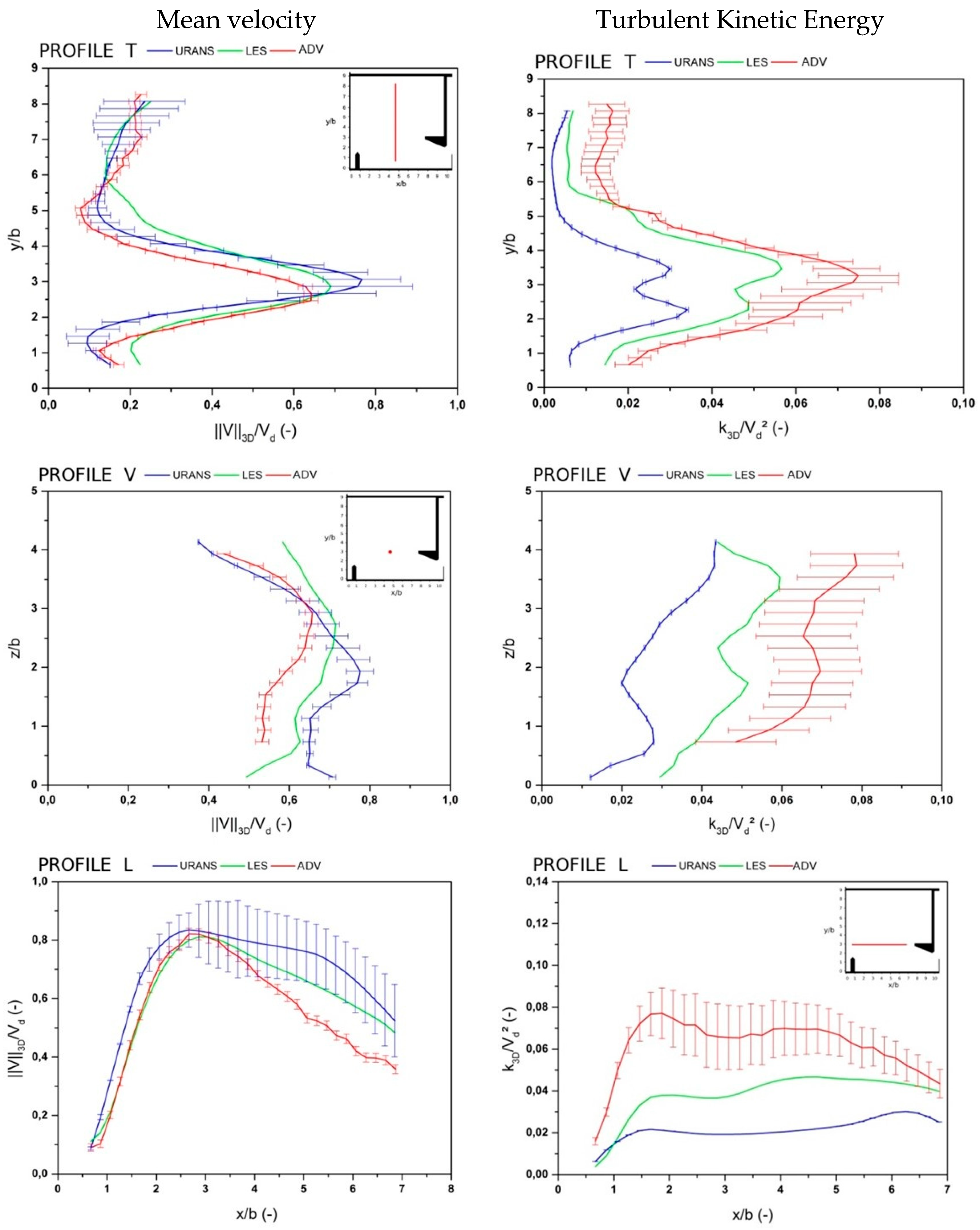
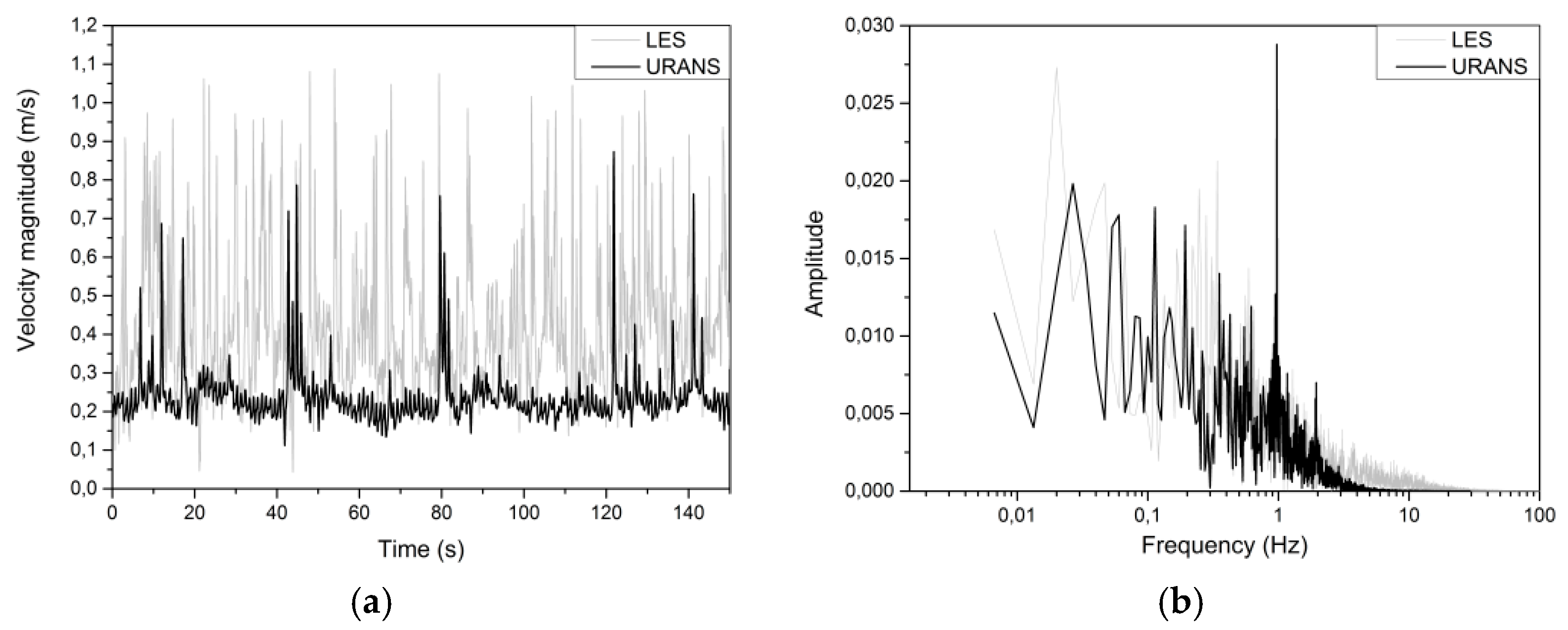
2.3. Validation
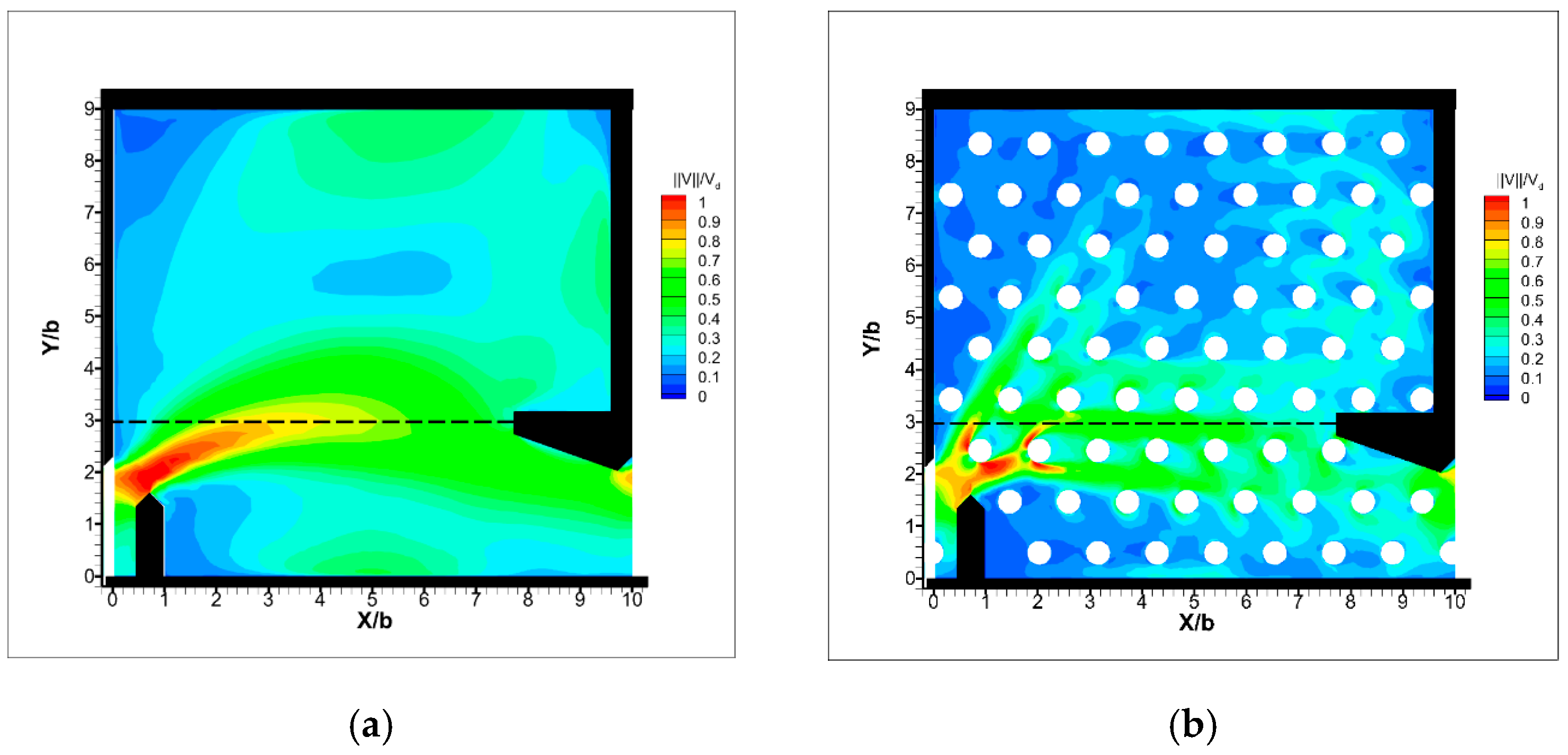
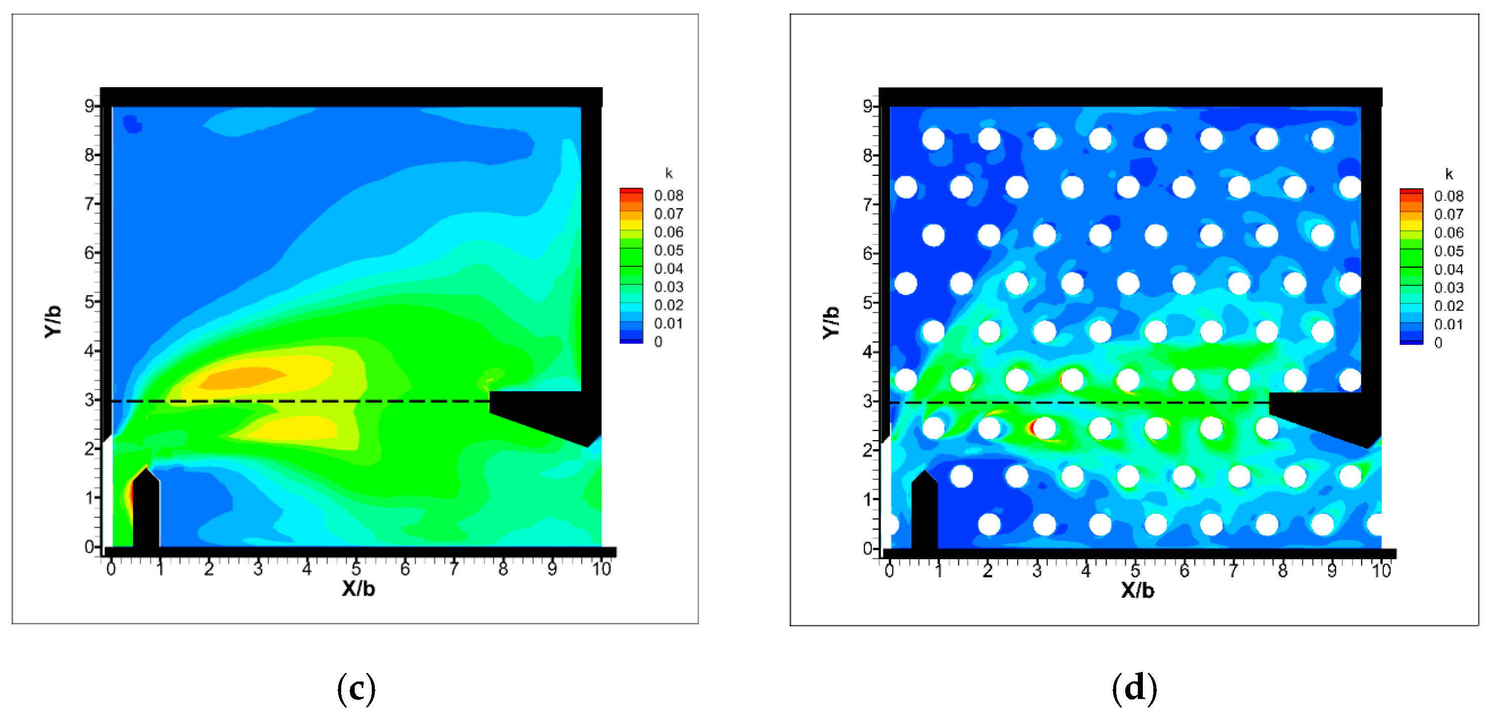
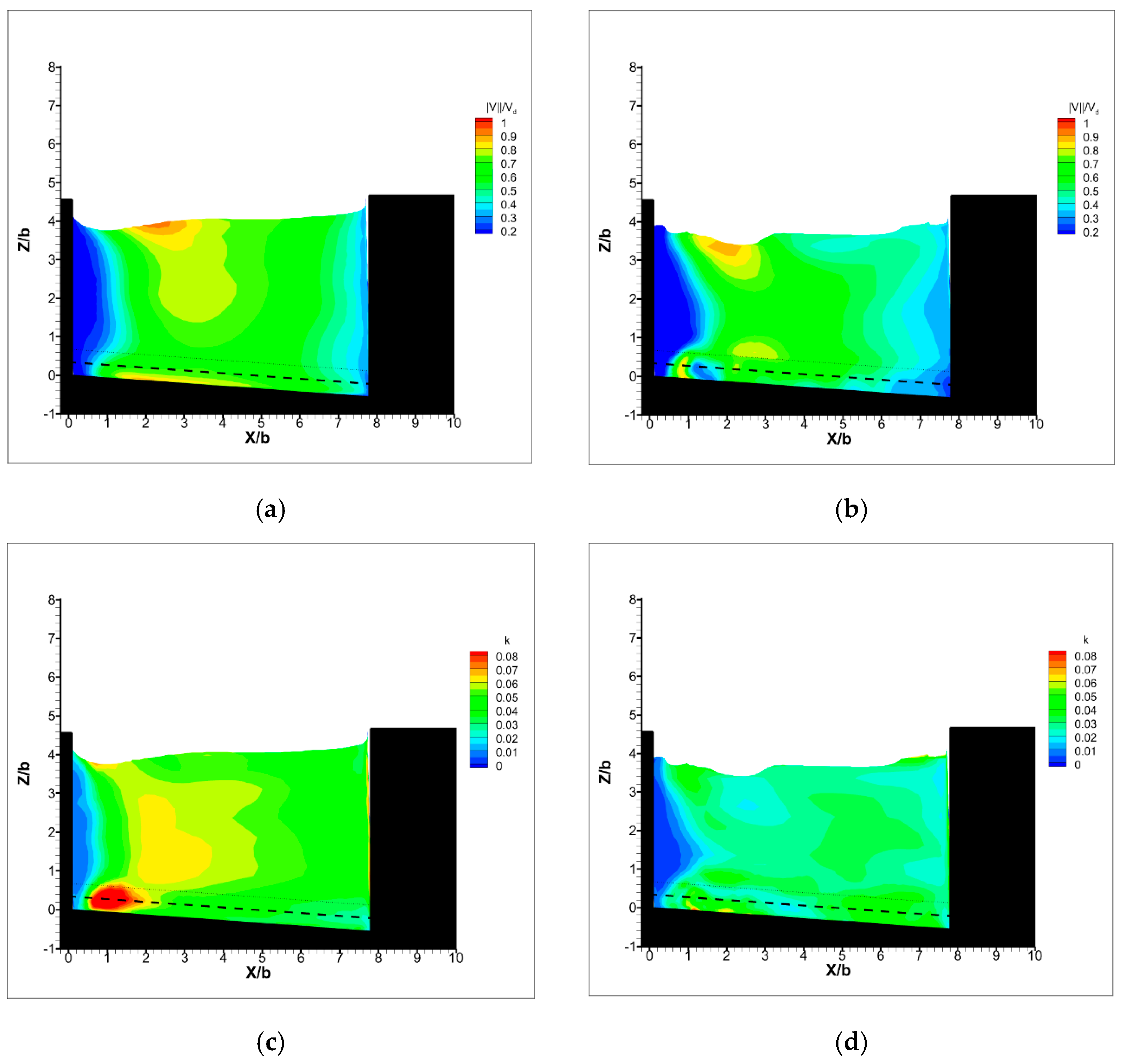
3. Results
4. Conclusions
Author Contributions
Funding
Data Availability Statement
Acknowledgments
Conflicts of Interest
Abbreviations
| VSF | vertical slot fishway |
| CFD | Computational Fluid Dynamics |
| URANS | Unsteady Reynolds-Averaged Navier–Stokes |
| LES | Large Eddy Simulation |
| VOF | volume of fluid |
| ADV | Acoustic Doppler Velocimeter |
References
- Wu, S.; Rajaratnam, N.; Katopodis, C. Structure of Flow in Vertical Slot Fishway. J. Hydraul. Eng. 1999, 125, 351–360. [Google Scholar] [CrossRef]
- Puertas, J.; Pena, L.; Teijeiro, T. Experimental Approach to the Hydraulics of Vertical Slot Fishways. J. Hydraul. Eng. 2004, 130, 10–23. [Google Scholar] [CrossRef]
- Liu, M.; Rajaratnam, N.; Zhu, D.Z. Mean Flow and Turbulence Structure in Vertical Slot Fishways. J. Hydraul. Eng. 2006, 132, 765–777. [Google Scholar] [CrossRef]
- Tarrade, L.; Texier, A.; David, L.; Larinier, M. Topologies and measurements of turbulent flow in vertical slot fishways. Hydrobiologia 2008, 609, 177–188. [Google Scholar] [CrossRef]
- Wang, R.; David, L.; Larinier, M. Contribution of experimental fluid mechanics to the design of vertical slot fish passes. Knowl. Manag. Aquat. Ecosyst. 2010, 396, 2. [Google Scholar] [CrossRef]
- Mallen-Cooper, M.; Zampatti, B.; Stuart, I.; Baumgartner, L. Innovative Fishways—Manipulating Turbulence in the Vertical Slot Design to Improve Performance and Reduce Cost; Technicol Report, Fishway Consult; Murray Darling Basin Authority: Sydney, NSW, Australia, 2008. [Google Scholar]
- Calluaud, D.; Pineau, G.; Texier, A.; David, L. Modification of vertical slot fishway flow with a supplementary cylinder. J. Hydraul. Res. 2014, 52, 614–629. [Google Scholar] [CrossRef]
- Zhao, H.; Xu, Y.; Lu, Y.; Lu, S.; Dai, J.; Meng, D. Numerical Study of Vertical Slot Fishway Flow with Supplementary Cylinders. Water 2022, 14, 1772. [Google Scholar] [CrossRef]
- Ballu, A.; Pineau, G.; Calluaud, D.; David, L. Experimental-Based Methodology to Improve the Design of Vertical Slot Fishways. J. Hydraul. Eng. 2019, 145, 04019031. [Google Scholar]
- Ballu, A. Étude Numérique et Expérimentale de L’écoulement Turbulent au Sein des Passes à Poissons à Fentes Verticales. Analyse de L’écoulement Tridimensionnel et Instationnaire. Ph.D. Thesis, Université de Poitiers, Poitiers, France, 2017. [Google Scholar]
- Bombač, M.; Rak, G.; Novak, G. Mathematical modeling of flow in vertical slot fishways. Acta Hydrotech. 2020, 33, 97–112. [Google Scholar] [CrossRef]
- Tarena, F.; Nyqvist, D.; Katopodis, C.; Comoglio, C. Computational fluid dynamics in fishway research—A systematic rewiew on upstream fish passage solutions. J. Ecohydraulics 2024, 10, 107–126. [Google Scholar] [CrossRef]
- Tarrade, L. Etude des Écoulements Turbulents dans les Passes à Poissons à Fentes Verticales: Adaptation aux Petites Espèces. Ph.D. Thesis, Université de Poitiers, Poitiers, France, 2007. [Google Scholar]
- Cea, L.; Pena, L.; Puertas, J.; Vázquez-Cendón, M.E.; Peña, E. Application of several depth-averaged turbulence models to simulate flow in vertical slot fishways. J. Hydraul. Eng. 2007, 133, 160–172. [Google Scholar] [CrossRef]
- Chorda, J.; Maubourguet, M.M.; Roux, H.; Larinier, M.; Tarrade, L.; David, L. Two-dimensional free surface flow numerical model for vertical slot fishways. J. Hydraul. Res. 2010, 48, 141–151. [Google Scholar]
- Bermúdez, M.; Puertas, J.; Cea, L.; Pena, L.; Balairón, L. Influence of pool geometry on the biological efficiency of vertical slot fishways. Ecol. Eng. 2010, 36, 1355–1364. [Google Scholar] [CrossRef]
- Bombač, M.; Novak, G.; Rodič, P.; Četina, M. Numerical and physical model study of a vertical slot fishway. J. Hydrol. Hydromechanics 2014, 62, 150–159. [Google Scholar] [CrossRef]
- Bombač, M.; Četina, M.; Novak, G. Study on flow characteristics in vertical slot fishways regarding slot layout optimization. Ecol. Eng. 2017, 107, 126–136. [Google Scholar] [CrossRef]
- Bousmar, D.; Zorzan, G.; Gillet, A.; Delhoulle, J.; Baugnée, A.; De Greef, J.C. Refurbishing an old fish pass: Physical and numerical modeling. In Proceedings of the River Flow, Lausanne, Switzerland, 3–5 September 2014; pp. 2427–2435. [Google Scholar]
- Zhang, D.; Qu, Y.; Shi, X.; Liu, Y.; Jiang, C. Design of a novel multislot and pool–weir combined fishway based on hydraulic properties analysis and fish-passage experiments. J. Hydraul. Eng. 2024, 150, 04024004. [Google Scholar] [CrossRef]
- Heimerl, S.; Hagmeyer, M.; Echteler, C. Numerical flow simulation of pool-type fishways: New ways with well-known tools. Hydrobiologia 2008, 609, 189–196. [Google Scholar] [CrossRef]
- Chang, W.; Lien, H.; Tsai, W.; Lai, J.; Guo, W.; Hu, T. 3D Flow Simulations In A Pool-weir-type Fishway In The Tonghou River. In Proceedings of the 33rd IAHR World Congress, Vancouver, BC, Canada, 9–14 August 2009. [Google Scholar]
- Barton, A.F.; Keller, R.J.; Katopodis, C. Verification of a numerical model for the prediction of low slope vertical slot fishway hydraulics. Australas. J. Water Resour. 2009, 13, 53–60. [Google Scholar] [CrossRef]
- Musall, M.; Schmitz, C.; Oberle, P.; Nestmann, F.; Henning, M.; Weichert, R. Analysis of flow patterns in vertical slot fishways. In Proceedings of the River Flow, Lausanne, Switzerland, 3–5 September 2014; pp. 2421–2426. [Google Scholar]
- An, R.; Li, J.; Liang, R.; Tuo, Y. Three-dimensional simulation and experimental study for optimising a vertical slot fishway. J. Hydro-Environ. Res. 2016, 12, 119–129. [Google Scholar] [CrossRef]
- Duguay, J.; Lacey, R.; Gaucher, J. A case study of a pool and weir fishway modeled with OpenFOAM and FLOW-3D. Ecol. Eng. 2017, 103, 31–42. [Google Scholar] [CrossRef]
- Umeda, Y.C.L.; de Lima, G.; Janzen, J.G.; Salla, M.R. One- and three-dimensional modelling of a vertical-slot fishway. J. Urban Environ. Eng. 2017, 11, 99–107. [Google Scholar]
- Stamou, A.I.; Mitsopoulos, G.; Rutschmann, P.; Bui, M.D. Verification of a 3D CFD model for vertical slot fish-passes. Environ. Fluid Mech. 2018, 18, 1435–1461. [Google Scholar] [CrossRef]
- Li, Y.; Wang, X.; Xuan, G.; Liang, D. Effect of parameters of pool geometry on flow characteristics in low slope vertical slot fishways. J. Hydraul. Res. 2019, 58, 395–407. [Google Scholar] [CrossRef]
- Quaranta, E.; Katopodis, C.; Comoglio, C. Effects of bed slope on the flow field of vertical slot fishways. River Res. Appl. 2019, 35, 656–668. [Google Scholar] [CrossRef]
- Fuentes-Pérez, J.F.; Silva, A.T.; Tuhtan, J.A.; García-Vega, A.; Carbonell-Baeza, R.; Musall, M.; Kruusmaa, M. 3D modelling of non-uniform and turbulent flow in vertical slot fishways. Environ. Model. Softw. 2018, 99, 156–169. [Google Scholar] [CrossRef]
- Ahmadi, M.; Kuriqi, A.; Nezhad, H.M.; Ghaderi, A.; Mohammadi, M. Innovative configuration of vertical slot fishway to enhance fish swimming conditions. J. Hydrodyn. 2022, 34, 917–933. [Google Scholar] [CrossRef]
- Tarrade, L.; Pineau, G.; Calluaud, D.; Texier, A.; David, L.; Larinier, M. Detailed experimental study of hydrodynamic turbulent flows generated in vertical slot fishways. Environ. Fluid Mech. 2011, 11, 1–21. [Google Scholar] [CrossRef]
- Fuentes-Pérez, J.F.; Quaresma, A.L.; Pinheiro, A.; Sanz-Ronda, F.J. OpenFOAM vs FLOW-3D: A comparative study of vertical slot fishway modelling. Ecol. Eng. 2022, 174, 106446. [Google Scholar] [CrossRef]
- Quaresma, A.L.; Pinheiro, A.N. Modelling of Pool-Type Fishways Flows: Efficiency and Scale Effects Assessment. Water 2021, 13, 851. [Google Scholar] [CrossRef]
- Quaresma, A.L.; Romão, F.; Pinheiro, A.N. A Comparative Assessment of Reynolds Averaged Navier–Stokes and Large-Eddy Simulation Models: Choosing the Best for Pool-Type Fishway Flow Simulations. Water 2025, 17, 686. [Google Scholar] [CrossRef]
- Celik, I.B.; Ghia, U.; Roache, P.J.; Freitas, C.J. Procedure for estimation and reporting of uncertainty due to discretization in CFD applications. J. Fluids Eng. Trans. ASME 2008, 130, 078001. [Google Scholar]
- Schlichting, H.; Gersten, K. Boundary-Layer Theory, 9th ed.; Springer: Berlin/Heidelberg, Germany, 2017. [Google Scholar]
- Chassaing, P. Turbulence en Mécanique des Fluides: Analyse du Phénomène en vue de sa Modélisation à L’usage de L’ingénieur; Cépaduès-Editions: Toulouse, France, 2000. [Google Scholar]
- Piomelli, U.; Balaras, E. Wall-layer models for large-eddy simulations. Annu. Rev. Fluid Mech. 2002, 34, 349–374. [Google Scholar] [CrossRef]
- Goring, D.G.; Nikora, V.I. Despiking Acoustic Doppler Velocimeter Data. J. Hydraul. Eng. 2002, 128, 117–126. [Google Scholar] [CrossRef]
- Joint Committee for Guides in Metrology—Guide to the Expression of Uncertainty in Measurement (JCGM-2023). Available online: https://www.bipm.org/documents/20126/2071204/JCGM_GUM-1.pdf/74e7aa56-2403-7037-f975-cd6b555b80e6 (accessed on 27 February 2025).
- Beaulieu, C.; Pineau, G.; Ballu, A.; David, L. Estimation process of uncertainties measurement in a research laboratory: Con-tribution and perspectives. Example of a research laboratory in hydrology for aquatic environments. In Proceedings of the 17th International Congress of Metrology, Paris, France, 21–24 September 2015. [Google Scholar]


| Profile T | Profile V | Profile L | |||||
|---|---|---|---|---|---|---|---|
| (%) | (-) | (%) | (-) | (%) | (-) | ||
| URANS | 28.8 | 0.87 | 15.7 | 0.56 | 22.6 | 0.92 | |
| LES | 28.5 | 0.89 | 14.2 | 0.91 | 11.3 | 0.95 | |
| URANS | 66.0 | 0.95 | 55.4 | 0.55 | 65.0 | 0.26 | |
| LES | 28.8 | 0.98 | 27.0 | 0.74 | 38.0 | 0.64 | |
Disclaimer/Publisher’s Note: The statements, opinions and data contained in all publications are solely those of the individual author(s) and contributor(s) and not of MDPI and/or the editor(s). MDPI and/or the editor(s) disclaim responsibility for any injury to people or property resulting from any ideas, methods, instructions or products referred to in the content. |
© 2025 by the authors. Licensee MDPI, Basel, Switzerland. This article is an open access article distributed under the terms and conditions of the Creative Commons Attribution (CC BY) license (https://creativecommons.org/licenses/by/4.0/).
Share and Cite
Pineau, G.; Ballu, A.; David, L.; Calluaud, D. Numerical Simulation of the Unsteady 3D Flow in Vertical Slot Fishway—The Impact of Macro-Roughness. Water 2025, 17, 1088. https://doi.org/10.3390/w17071088
Pineau G, Ballu A, David L, Calluaud D. Numerical Simulation of the Unsteady 3D Flow in Vertical Slot Fishway—The Impact of Macro-Roughness. Water. 2025; 17(7):1088. https://doi.org/10.3390/w17071088
Chicago/Turabian StylePineau, Gérard, Aurélien Ballu, Laurent David, and Damien Calluaud. 2025. "Numerical Simulation of the Unsteady 3D Flow in Vertical Slot Fishway—The Impact of Macro-Roughness" Water 17, no. 7: 1088. https://doi.org/10.3390/w17071088
APA StylePineau, G., Ballu, A., David, L., & Calluaud, D. (2025). Numerical Simulation of the Unsteady 3D Flow in Vertical Slot Fishway—The Impact of Macro-Roughness. Water, 17(7), 1088. https://doi.org/10.3390/w17071088