Flow Pattern and Turbulent Kinetic Energy Analysis Around Tandem Piers: Insights from k-ε Modelling and Acoustic Doppler Velocimetry Measurements

Abstract

This study investigated the distribution and dynamics of the Turbulent Kinetic Energy (TKE) around a group of three tandem piers using a combination of numerical simulations and experimental measurements. The Volume of Fluid (VOF) method, coupled with the k-$\epsilon$ turbulence model, was implemented in ANSYS FLUENT to replicate the free-surface flow conditions. An experimental validation was conducted using Acoustic Doppler Velocimetry (ADV) to assess the model’s capability at capturing the turbulence characteristics. While the model effectively reproduced the near-bed turbulence, it consistently underestimated the TKE magnitudes across the flow domain, particularly in regions of strong vortex-induced turbulence. Discrepancies emerged in the confined regions between the piers, where the velocity profiles were overestimated at the surface and underestimated near the bed and mid-depth, impacting the TKE predictions. Despite these inconsistencies, the general pattern of the TKE distribution aligned with the experimental trends, though the absolute values remained underestimated due to the inherent limitations of the k-$\epsilon$ model. The model’s performance in less turbulent regions demonstrated improved accuracy, reinforcing its applicability for moderate turbulence simulations. To further examine the interaction between vortex structures and the TKE, velocity distributions were analyzed at three specific depths (z/h = 0.15, 0.4, and 0.62). The findings showed the critical role of vortex shedding in TKE generation and dissipation, with notable variations in the turbulence intensity influenced by structural confinement effects. This study offers a novel, high-resolution evaluation of the k-ε model’s ability to predict TKE distributions around tandem piers, using spatially detailed comparisons with the experimental data. Unlike previous studies that broadly acknowledged the model’s limitations, this work systematically identifies the specific regions, particularly vortex-dominated zones, where its predictive accuracy significantly degrades.

1. Introduction

Bridges are among the most influential structures affecting the hydraulics and morphology of rivers, and bridge engineers must have a thorough understanding of scour development, as it is a major cause of bridge failures, often resulting from the flow processes around bridge piers and abutments [1,2,3]. Moreover, bridge construction can lead to backwater issues, especially during floods; therefore, accurately estimating the rise in the water surface level due to bridge constrictions and determining the maximum backwater height are essential considerations in bridge design [4,5]. Consequently, any damage to these structures raises significant concerns for civil engineers and bridge designers [6].

Numerical models are essential tools for estimating the hydrodynamic characteristics of flow and analyzing the related issues. They enable researchers and engineers to quickly evaluate various scenarios and develop effective solutions for water flow management, flood control, and predicting the behaviour of hydraulic systems [7]. Conversely, recent developments in three-dimensional numerical simulations that can resolve eddies for analyzing the flow around bridge piers and abutments [8,9,10,11,12,13,14] have shown the ability to offer a comprehensive understanding of not only the mean flow characteristics and turbulence statistics, but also the unsteady dynamics of coherent structures that are vital in bed erosion processes.

Investigations into the turbulence around obstacles originated from laboratory experiments [15,16,17]. While there is a wealth of research concerning flow behaviour and sediment erosion in steady currents, the number of studies that have delved into the three-dimensional numerical modelling of these processes remains relatively small [18,19,20,21]. Moreover, most of these studies have concentrated on flow behaviours over flat, rigid surfaces [22,23]. These studies have also included an assessment of the mean flow field and turbulence statistics surrounding piers, along with visualization experiments on coherent structures, like horseshoe vortex systems and billow wake vortices. These investigations have deepened our comprehension of how these structures affect fluid behaviour, which is essential for the effective design and analysis of hydraulic systems [24,25,26,27,28,29]. However, these methods are limited in their ability to capture three-dimensional instantaneous flow fields and the associated bed shear stress distributions.

For over 15 years, the research has concentrated on simulating turbulent flows in natural rivers. A key early model by Sinha and Sotiropoulos [30] utilized a three-dimensional multi-block approach to simulate a 2.5-mile stretch of the Columbia River, achieving strong agreement with laboratory-scale results through steady RANS simulations using the k-ε model.

When an obstacle is placed in the flow path, the surrounding flow transforms from a uniform one-dimensional state into a complex three-dimensional structure due to the flow separation, which significantly affects the boundary layer. The authors of [22,31], utilizing experimental and computational investigations alongside the FSI-CURVIB method, examined the clear-water scour around various bridge pier shapes, including cylindrical, square, and diamond configurations. The study revealed that a hydrodynamic model grounded in Reynolds-averaged Navier–Stokes (URANS) equations, coupled with the k-ε turbulence model, can accurately predict the scour for diamond piers. However, it tends to underestimate the scour for blunt-edged piers due to challenges associated with the vortex resolution.

Flow modelling using FLUENT Computational Fluid Dynamics (CFD) and various turbulence models has been conducted by Ali and Karim [1]. In their study, FLUENT CFD was employed to simulate the flow around a circular cylinder, analyzing the rigid beds and the dimensions of the scour holes. Their study formulated an expression for the time-dependent scour depth, which is influenced by three dimensionless parameters: the pile number, sediment size number, and duration time number. This expression was subsequently validated against both laboratory and field data. Xiong and Cai [32] conducted CFD simulations and analyses of bridge scour development using a dynamic mesh updating technique. This study employed the k-ε turbulence model in CFD simulations to assess the transient shear stress, vital for analyzing the sediment motion during scour around bridge piers. The results showed that the k-$\epsilon$ turbulence model can effectively predict the flow fields and scour profiles, validated by comparisons with the experimental data, and demonstrates reliability in analyzing the scour behaviour across different pier types. The study conducted by Guemou and Seddini [33] examined the behaviour of sediment particles and the simulation of the turbulent flow around bridge piers. This study explored the impact of an aerodynamic design on the bed shear stress around bridge piers, focusing on the local scour risks. Utilizing the Finite Volume Method (FVM) and detached eddy simulation (DES), the results indicated that a rounded-nosed pier should not exceed 2.5 times its width to effectively minimize the bed shear stress. Also, the simulation of the rotational flow and flow reattachment length over a backward-facing step using Fluent software (volume 15317) was investigated by Soori and Hajikandi [34]. In this study, various turbulence models, including $RNGk\text{-}\epsilon$, Realizable $k\text{-}\epsilon$, and $k\text{-}\omega ,$ were employed. The results indicated that the $RNG$ k-ε turbulence model exhibited better agreement with the experimental data. Moreover, Svsndl and Suresh [35] investigated the local scour around bridge piers, a major cause of bridge failures, using CFD simulations with Fluent and the k-ε model. The scour depth was estimated through empirical formulas and validated experimentally, with the simulation results aligning with the experimental data, demonstrating the effectiveness of CFD for understanding the flow behaviour around bridge piers. Additionally, three-dimensional flow modelling around cylindrical piers in river meanders was conducted using ANSYS FLUENT, specifically focusing on a $180°$ curve, with piers featuring a $21°$ slope and a diameter of $5\mathrm{c}\mathrm{m}$, as studied by Lahsaei and Vaghefi [36]. The results demonstrated that the model can effectively simulate the flow patterns influenced by the relative radius of the curvature and the arrangement of the piers. It was found that increasing the curvature leads to a reduction in the tangential velocity. Additionally, the maximum secondary flow strength varied at different locations based on the orientation of the piers relative to the flow direction. Ahmed and Ismael [37] used the CFD–Fluent (k-ε) turbulence model to simulate the water flow and Turbulent Kinetic Energy (TKE) around two pier designs, an upstream-facing aero-foiled shaped pier (US-FASP) and a downstream-facing aero-foiled shaped pier (DS-FASP), alongside a circular pier. The results showed that the DS-FASP design was the most effective, promoting a smooth flow and resulting in the lowest TKE. The k-ε model effectively captured the wake vortex shape, demonstrating a strong agreement with the experimental data, and highlighting the DS-FASP’s superior performance for flow dynamics and turbulence characteristics.

Acoustic Doppler Velocimetry (ADV) and CFD models are powerful tools used in the study of fluid flow and turbulence. ADV is an experimental technique that employs the Doppler effect to measure the velocity of particles suspended in a fluid, providing high-resolution, three-dimensional velocity data in real-time. This method is particularly valuable for capturing the complex flow structures and dynamics in various environments, such as around bridge piers or in river systems [38,39,40,41]. On the other hand, CFD models utilize numerical algorithms and computational power to simulate the fluid flow based on the governing equations of fluid mechanics [42,43,44,45,46,47]. They have been used to conduct experimental and numerical investigations of three-dimensional (3D) flow patterns around intact and damaged bridge piers using Acoustic Doppler Velocimetry (ADV), Particle Image Velocimetry (PIV), and CFD simulations. ADV has been employed for flow velocity measurements, which have been validated using PIV. Numerical modelling with SSIIM (Sediment Simulation in Intakes with Multiblock Option) software has demonstrated a strong correlation with the experimental data. The results have indicated that the presence of bridge piers shift the location of the maximum bed shear stress toward the mid-channel, increasing it by 72%, while also causing significant water level variations both upstream and downstream.

These models can replicate intricate flow patterns, predict turbulence behaviour, and assess the interaction between fluids and structures under varying conditions. When used in conjunction, ADV and CFD can enhance our understanding of fluid dynamics by validating the simulation results with the empirical data, thereby improving scour predictions and informing engineering designs of hydraulic structures [14,41,47,48,49,50].

Accurately predicting the TKE in complex flow environments remains a challenge in hydraulic engineering, particularly around bridge piers, where the turbulence-driven scour and structural stability are critical concerns. This study examines the TKE distributions around three tandem square piers using a Volume of Fluid (VOF)-based k-ε turbulence model, with the numerical results validated against high-resolution experimental data obtained via ADV. While the k-ε model effectively captures the global velocity field and overall turbulence structure, its limitations become evident in regions dominated by intense vortex shedding and wake interactions. Specifically, the model underpredicts the TKE magnitudes in high-shear regions near the piers, where complex turbulence production and dissipation mechanisms drive energy exchange. These discrepancies reflect the model’s inability to resolve energy-containing eddies and anisotropic turbulence effects, which are critical for accurately predicting the flow-induced forces and sediment transport.

The findings of this study show a key limitation of the k-$\epsilon$ turbulence model for accurately capturing the TKE dynamics, particularly in regions of strong turbulence production and dissipation. While the model remains a widely used engineering tool due to its computational efficiency for large-scale simulations, its inability to precisely resolve the TKE distribution emphasises the need for higher-fidelity turbulence models, such as a Large-Eddy Simulation (LES) or Direct Numerical Simulation (DNS), for applications requiring detailed turbulence energy estimates. However, the computational cost of these advanced models often limits their feasibility for use in full-scale parametric studies. Previous studies have indicated the low accuracy of standard turbulence models for predicting the TKE [51,52], yet this gap has not been sufficiently addressed in the existing research.

This study presents a novel evaluation framework that quantifies the specific regions and flow conditions where the k-$\epsilon$ model fails to capture the TKE accurately, particularly under highly turbulent conditions generated by hydraulic structures. This approach goes beyond general performance comparisons by offering a detailed spatial and functional analysis of the model’s predictive limitations. Such an analysis has not been explicitly conducted in earlier studies. This study builds on previous knowledge to further assess the predictive limitations of the k-$\epsilon$ model and its implications for engineering applications. Despite its limitations, the k-$\epsilon$ model was selected for this study because it enables efficient simulations across multiple operating conditions while still providing reasonable accuracy for predicting bulk flow characteristics, including the mean velocity profiles and recirculation zones. This balance between computational feasibility and predictive capability is crucial in engineering applications, such as scour control, hydraulic structure optimization, and sediment transport modelling, where large-scale simulations are required. The novelty of this work lies in its focused investigation of the TKE under structure-induced turbulence and its contribution to refining turbulence modelling strategies for practical, large-scale hydraulic simulations. This study, therefore, shows the trade-off between computational efficiency and turbulence resolution in standard turbulence modelling approaches, contributing to the development of improved methodologies for capturing turbulence-driven flow interactions in hydraulic structures.

2. Numerical Model

2.1. Hydrodynamic Model

Setting up a numerical model in ANSYS Fluent involves careful attention to mesh quality, boundary conditions, physical models, solver settings, and post-processing techniques to effectively address complex fluid dynamics problems. This section details the simulation and CFD processes in Fluent, highlighting the numerical schemes used and the computational grid properties for each case. Given that ANSYS Fluent employs the FVM, it divides the solution domain into discrete control volumes to solve mass and momentum conservation equations. Over the last few decades, there has been an increasing focus on numerical models for the study of turbulent flows.

The three-dimensional Navier–Stokes equations, along with the continuity and momentum equations, can be expressed as follows [53,54]:

Continuity equation:

$${\displaystyle \frac{\partial \rho }{\partial t}}+{\displaystyle \frac{\partial }{\partial x}}\left(\rho u\right)+{\displaystyle \frac{\partial }{\partial y}}(\rho v)=0$$

(1)

Momentum equations:

$$\begin{gathered} {\displaystyle \frac{\partial }{\partial t}}\left(\rho u\right)+\nabla ·\left(\rho uV\right)=-{\displaystyle \frac{\partial P}{\partial x}}+{\displaystyle \frac{{\partial \tau }_{xx}}{\partial x}}+{\displaystyle \frac{{\partial \tau }_{yx}}{\partial \mathrm{y}}}+\rho f_x \\ {\displaystyle \frac{\partial }{\partial t}}\left(\rho v\right)+\nabla ·\left(\rho vV\right)=-{\displaystyle \frac{\partial P}{\partial y}}+{\displaystyle \frac{{\partial \tau }_{xy}}{\partial x}}+{\displaystyle \frac{{\partial \tau }_{yy}}{\partial \mathrm{y}}}\rho f_y \end{gathered}$$

(2)

where $\rho$ is the fluid density; $t$ is time; $u$ and $v$ are the velocity components in the $x$ and $y$ directions, respectively; $V$ is the velocity vector; and $P$ is pressure. The terms ${\tau }_{xx}$ and ${\tau }_{yy}$ represent the normal stresses caused by viscosity in the $x$ and $y$ directions, respectively; while ${\tau }_{xx}$, ${\tau }_{xy}$, ${\tau }_{yy},$ and ${\tau }_{yx}$ denote the shear stresses, which describe how motion in one direction influences stress in another direction. Additionally, $f_x$ and $f_y$ are the body force components per unit volume in the $x$ and $y$ directions, respectively. The momentum equations govern momentum conservation in the x and y directions. The terms $\partial \left(\rho u\right)/\partial t$ and $\partial \left(\rho v\right)/\partial t$ represent the rate of momentum change over time, while $\nabla ·\left(\rho uV\right)$ and $\nabla ·\left(\rho vV\right)$ account for momentum convection. The pressure gradients $\partial P/\partial x$ and $\partial P/\partial y$ drive fluid motion, and the terms $\rho f_x$ and $\rho f_y$ represent external body forces like gravity.

By discretizing the flow equations within the control volume, the partial differential equations are transformed into a system of algebraic equations. Subsequently, these algebraic equations are solved numerically to derive the solution field.

In this study, the standard k-$\epsilon$ model is employed for simulation purposes. To address the perturbation equations associated with this model within ANSYS FLUENT 2022 R2 software, the solutions to Equations (3) and (4) are utilized to compute the values of Turbulent Kinetic Energy and Turbulent Dissipation Rate for each iteration, respectively [34,54,55,56].

$k-Equation:$

$${\displaystyle \frac{\partial \left(\rho k\right)}{\partial t}}+{\displaystyle \frac{\partial }{{\partial }_x}}\left(\rho ku\right)+{\displaystyle \frac{\partial }{{\partial }_y}}\left(\rho kv\right)={\displaystyle \frac{\partial }{{\partial }_x}}\left[\left(\mu +{\displaystyle \frac{{\mu }_t}{{\sigma }_k}}\right){\displaystyle \frac{\partial k}{{\partial }_x}}\right]+{\displaystyle \frac{\partial }{{\partial }_y}}\left[\left(\mu +{\displaystyle \frac{{\mu }_t}{{\sigma }_k}}\right){\displaystyle \frac{\partial k}{{\partial }_y}}\right]+G_k+G_b-\rho \epsilon -Y_M+S_K$$

(3)

$\epsilon -Equation:$

$${\displaystyle \frac{\partial \left(\rho \epsilon \right)}{\partial t}}+{\displaystyle \frac{\partial }{{\partial }_x}}\left(\rho \epsilon u\right)+{\displaystyle \frac{\partial }{{\partial }_y}}\left(\rho \epsilon v\right)={\displaystyle \frac{\partial }{{\partial }_x}}\left[\left(\mu +{\displaystyle \frac{{\mu }_t}{{\sigma }_{\epsilon }}}\right){\displaystyle \frac{\partial \epsilon }{{\partial }_x}}\right]+{\displaystyle \frac{\partial }{{\partial }_y}}\left[\left(\mu +{\displaystyle \frac{{\mu }_t}{{\sigma }_{\epsilon }}}\right){\displaystyle \frac{\partial \epsilon }{{\partial }_y}}\right]+{\rho C}_1{S}_{\epsilon }-{\rho C}_2{\displaystyle \frac{{\epsilon }^2}{k+\sqrt{v\epsilon }}}{{+C}_{1\epsilon }{\displaystyle \frac{\epsilon }{k}}{C}_{3\epsilon }{G}_b+S}_{\epsilon }$$

(4)

where $\mu$ is the molecular viscosity, ${\mu }_t$ is the turbulent viscosity, ${\sigma }_k$ is the turbulent Prandtl number for k, and $P_k$ represents the production of TKE due to velocity gradients. The parameter ${\sigma }_{\epsilon }$ is the turbulent Prandtl number for ${\sigma }_{\epsilon }$, while $C_{1\epsilon }$, $C_{2\epsilon },$ and $C_{3\epsilon }$ are model constants for the dissipation rate equation. Additionally, $G_k$ represents the mean velocity gradient, and $G_b$ accounts for hydrodynamic effects, and ${\displaystyle \frac{\partial \left(\rho k\right)}{\partial t}}$ and ${\displaystyle \frac{\partial \left(\rho \epsilon \right)}{\partial t}}$ represent the rate of change in TKE over time and the turbulent dissipation rate over time, respectively [57].

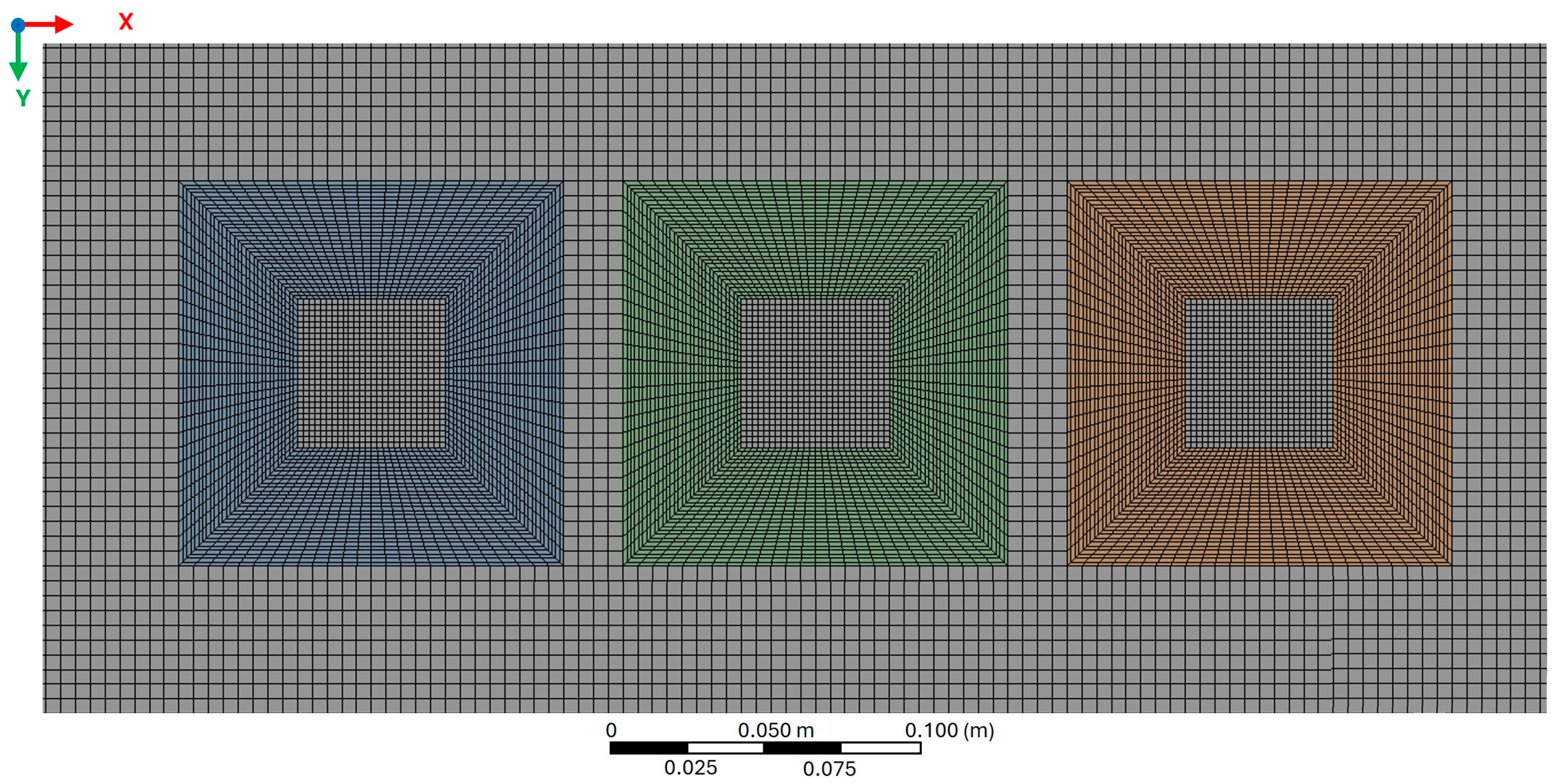
2.2. Numerical Setup

Research into the flow mechanisms around bridge piers is ongoing, with numerical models frequently employed to study turbulent flows. Observations have indicated that even simple hydraulic structures can produce complex flow patterns [58]. The primary aim of simulating flow around bluff bodies like bridge piers is to assess bed shear stress and predict the resulting scour hole [33]. Minor geometric adjustments can lead to considerable turbulence effects [59]. The geometric layout and smooth boundary conditions for a numerical simulation with a total flow domain length of $1.35\mathrm{m}$ were chosen to facilitate meaningful comparisons with experimental results [14]. In the experimental setup, the distance from the inlet to the first pier was established at $3\mathrm{m}$ to ensure fully developed flow before reaching the piers. A uniform upstream velocity of $0.76\mathrm{m}/\mathrm{s}$ was maintained, with a water discharge of ${0.072\mathrm{m}}^3/\mathrm{s}$ and a consistent flow depth of $0.21\mathrm{m}$ recorded throughout the flume prior to adding pier blocks.

Figure 1 shows three uniform mesh sizes (0.1 m, 0.01 m, and 0.009 m) that were tested across the domain. The largest mesh (0.1 m), with 31,830 nodes and 25,114 elements, was found insufficient for resolving flow details, especially near the piers, and further refinement was necessary to accurately capture the high-turbulence regions. To optimize computational efficiency without compromising accuracy, a hybrid meshing approach was adopted. However, a structured hexahedral mesh (0.005 m) was applied to the general domain, while a finer mesh (0.001 m) was used around the piers to capture vortex structures and flow separation effects (Figure 2). A multi-zone meshing approach was adopted, resulting in approximately 2.3 million nodes and 2.23 million elements, with a standard element size of 0.005 m and a finer size of 0.001 m near the piers to accurately capture turbulent boundary layer. Also, for boundary conditions, a velocity inlet was applied at the upstream boundary based on experimental flow conditions, while a pressure outlet was set at the downstream boundary to allow for natural flow development. No-slip conditions were imposed on the piers and channel walls to account for shear effects, ensuring a realistic flow representation and numerical stability.

The dimensionless wall distance, $Y^{+}$, is a critical parameter for evaluating wall functions, as expressed in Equation (5), where $y$ denotes the distance from the wall and $U_{\tau }$ signifies the friction velocity, as outlined in Equation (6) [60,61]. Consequently, a value of $Y=0.0019$ was selected to ensure accurate representation near the wall.

$$Y={\displaystyle \frac{Y^{+}}{U_{\tau }v}}$$

(5)

where the distance from the wall (y) is 0.0032 m, the wall shear velocity ($U_{\tau })$ is 0.012765 m/s, and $v$ represents the kinematic viscosity of the fluid. Based on these parameters, the $y^{+}$ value is 40, which falls within the appropriate range for turbulence modelling and wall treatment considerations.

$$U_{\tau }=\sqrt{{\displaystyle \frac{\frac{1}{2}·{0.058·Re}_l^{-0.2}·\rho {·U}_{\infty }^2}{\rho }}}$$

(6)

Additionally, the VOF method was implemented for analyzing multiphase flows, ensuring an air-to-water depth ratio of at least 0.5 to maintain smooth simulations and prevent issues like water surface breaking or sloshing.

The simulation in this study utilized a time step size of 0.005 s, comprising 20 iterations per step, in accordance with the Courant criterion to ensure accuracy and stability while avoiding divergence. Pressure-based solvers with coupled schemes were employed, specifically using a SIMPLE-type pressure–velocity coupling algorithm, which is an effective alternative to density-based and segregated pressure-based algorithms. This coupled approach was crucial for handling transient flows, particularly in scenarios with low-quality meshes or longer time steps typical of implicit numerical methods.

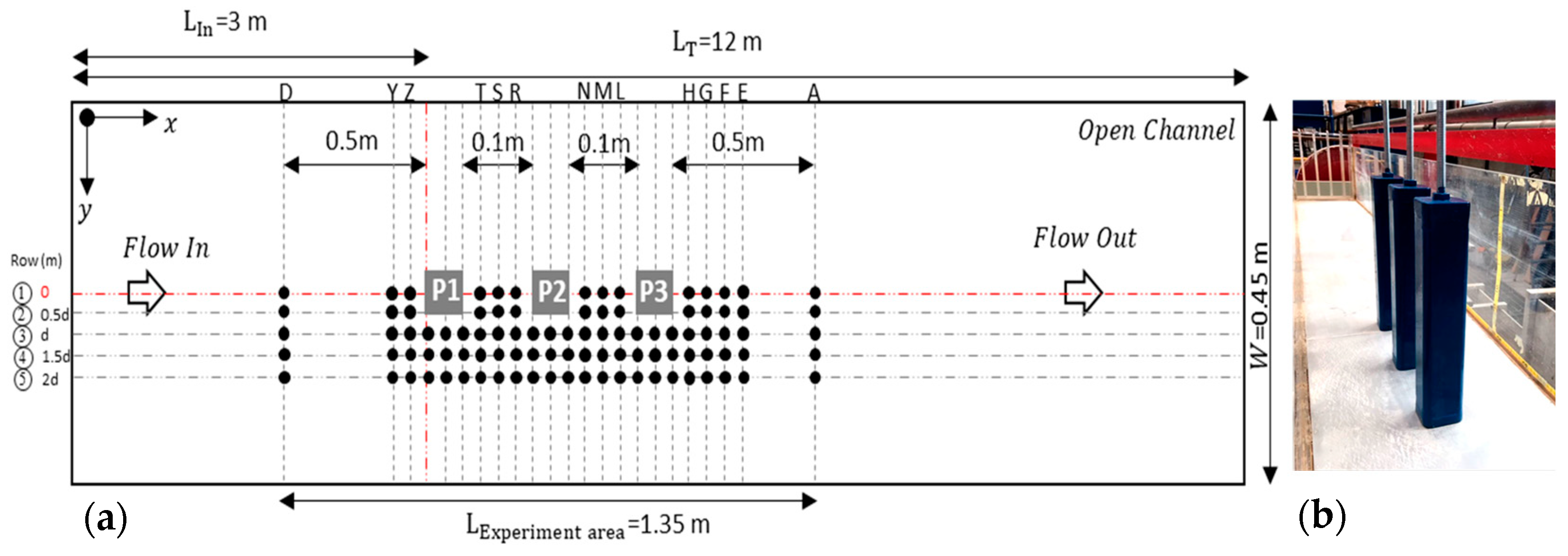
3. Experimental Setup

3.1. Hydraulic Model

Model verification was conducted using the experimental setup described by Ikani and Pu [40]. The setup featured a rectangular flume with dimensions of $12\mathrm{m}$ in length, $0.45\mathrm{m}$ in width, and $0.5\mathrm{m}$ in height. The channel was equipped with a fixed bed that had a slope $\left(S_0\right)$ of 0.0033, and was constructed from smooth stainless steel to minimize friction and turbulence around the piers. The flat square piers, each measuring $0.05\times 0.05\mathrm{m}$, were positioned at a distance of $2d$ ($d=0.05\mathrm{m}$) from one another and centred within the channel width. All piers were placed more than $6\mathrm{m}$ from channel inflow to ensure the elimination of inlet turbulence before reaching the measured location. The approach flow conditions were characterized by the approach flow depth ${(h}_0)$, Froude number (${Fr}_0=u_0/\sqrt{g{h}_0}$), and velocity ($u_0=Q_0/B{h}_0$), where Q₀; represents the discharge, B is the channel width, and g is the acceleration due to gravity. Figure 3b illustrates the side view of the flume along with the positioning of the bridge piers used in the experiments. The experiment utilized flow rate $\left(Q_0\right)$ of 0.072 $\mathrm{m}³/\mathrm{s}$, an approach flow depth ${(h}_0)$ of $0.21\mathrm{m}$, and an average velocity $\left(u_0\right)$ of $0.76\mathrm{m}/\mathrm{s}$.

Furthermore, to minimize boundary effects, the flume width (0.45 m) was chosen based on the ratio of flow width to channel width, which remained below 0.1, to make sure there were minimal wall-induced disturbances [62]. The pier spacing was also designed to minimize boundary influences and comparisons of velocity fluctuations confirmed a good agreement between experimental and numerical results, according to Ikani et al. [40].

During the experiments, flow characteristics around three square bridge piers were measured using ADV. In the study by [14], flow characteristics were examined at 60 different locations, as shown in Figure 3a.

3.2. Acoustic Doppler Velocimetry (ADV)

ADV is an essential tool in hydrodynamics, which is capable of precisely measuring 3D flow velocities by utilizing the Doppler shift principle within flows [63]. To evaluate the flow characteristics, velocity data were measured using a Nortek side-looking ADV (i.e., via Vectrino+ software). The instrument was strategically placed within the central cross-sectional area of the flume, $3\mathrm{m}$ downstream from the channel’s entrance (Figure 4). The data collection involved recording velocity datasets at each measured point for 5 min, with a set sampling frequency of $100\mathrm{H}\mathrm{z}$.

To ensure accuracy and precision, the ADV probes re-alignment method proposed by previous studies [55,64] was implemented to ensure the profile’s locational precision and to enhance data quality. ADV reveals the flow velocity by emitting and receiving acoustic signals. In bistatic mode configuration, the Doppler frequency shift $f_D$, is calculated from the emitted frequency $f_e$, received frequency $f_r$, celerity $c$, and velocities of the emitter $V_e$ and receiver $V_r$ relative to the moving fluid. The relationship is described by Equation (7) [65]:

$$f_D={\displaystyle \frac{f_e}{c}}\left(V_e+V_r\right)$$

(7)

Background noise can significantly affect measurement accuracy by altering the signal-to-noise ratio (SNR) and causing un-intended oscillations in datasets. This is a particularly serious issue for vertical velocity measurement, which is sensitive to noise. In Nortek ADV, two probes are used to measure two duplicate vertical velocities, with their averaged value used to improve SNR. Component velocities in the longitudinal $U$, transverse $V$, and vertical $W$ directions are integrated using angular discrepancies between the emitter, receiver, and the moving target. These velocities are formulated by

$$V_H=U·\cos \left(b\right)+V·\sin \left(b\right)$$

(8)

$$V_r=V_H·\sin \left(a\right)+W·\cos \left(a\right)=U·\sin \left(a\right)\cos \left(b\right)+V·\sin \left(a\right)\sin \left(b\right)+W·\cos \left(a\right)$$

(9)

where $a$ is defined as the angular difference between the direction of moving target and the receiver, with the emitter as the reference point. This angle quantifies the component of the target’s motion towards or away from the receiver and directly influences the observed Doppler shift. $b$ represents the angular difference between the probe emitter and the receiver. It is instrumental for resolving the horizontal velocity into its longitudinal and transverse components. The functions $\mathrm{c}\mathrm{o}\mathrm{s}\left(b\right)$ and $\mathrm{s}\mathrm{i}\mathrm{n}\left(b\right)$ facilitate the decomposition of these velocities relative to the probe’s orientation, thus affecting the accuracy of the measurements based on the spatial configuration of the ADV setup. Subsequently, the Doppler frequency shift, in terms of $U$, $V$, and $W,$ can be expressed as follows [64]:

$$f_D={\displaystyle \frac{f_e}{c}}[\sin \left(a\right)\cos \left(b\right)+V·\sin \left(a\right)\sin \left(b\right)+W(1+\cos \left(a\right))]$$

(10)

On the other hand, advanced signal processing techniques, such as phase averaging and coherent structure identification, are instrumental for refining the data collected. These methods improve the SNR and enable the precise determination of flow velocities under complex surrounding conditions [66]. Hence, data collection was conducted by positioning the probe at the lowest point (0.005 m) and then moving it upward between sampling rounds. This approach consistently produced data with high correlations (more than 70%) and SNRs of 15% minimum, while reducing data error significantly. During the pre-processing of data, any velocity reading with a correlation value below 70% or an inadequate SNR value was re-recorded. Therefore, by following these careful data collection and handling strategies, including advanced signal processing techniques and thorough calibration protocols, the reliability of measurements could be maintained.

3.3. Uncertainty Analysis

A data uncertainty analysis was conducted for the ADV measurements to determine the accuracy and reliability of our findings. Before data collection, calibration tests were performed four times to validate the consistency of velocity profiles at the same location under undisturbed conditions (Locations D1, D2, D3, and D4). Figure 5 presents two of these tests (at D1 and D2) which were conducted to ensure accuracy and assess experimental fully developed flow.

The uncertainty was quantified using the standard deviation $\sigma$ of repeated measurements, calculated as ($x_1=0.76,x_2=0.755,x_3=0.765,\mathrm{a}\mathrm{n}\mathrm{d}{x}_4=0.758)$. The standard deviation of the repeated velocity measurements was calculated as 0.0042 m/s, indicating a low level of variability and high measurement consistency. Given the small deviation relative to the mean velocity ($0.7595\mathrm{m}/\mathrm{s}$), the uncertainty in the experimental data was minimal, suggesting reliable measurement accuracy. This low uncertainty reinforces the validity of the experimental setup and confirms that observed discrepancies between numerical and experimental results are more likely attributable to model assumptions rather than measurement errors.

$$\sigma =\sqrt{{\displaystyle \frac{1}{N-1}}{\sum }_{i=1}^N{\left(x_i-\overline{x}\right)}^2}$$

(11)

where $N$ is the number of measurements, $x_i$ is each individual measurement, and $\overline{x}$ is the mean of the measurements. The relative uncertainty was then calculated as

$$Uncertaintly=\left({\displaystyle \frac{\sigma }{Meanvelocity}}\right)\times 100$$

(12)

The results showed that the relative uncertainty was 0.55%, which was within acceptable range or error.

4. Results and Discussion

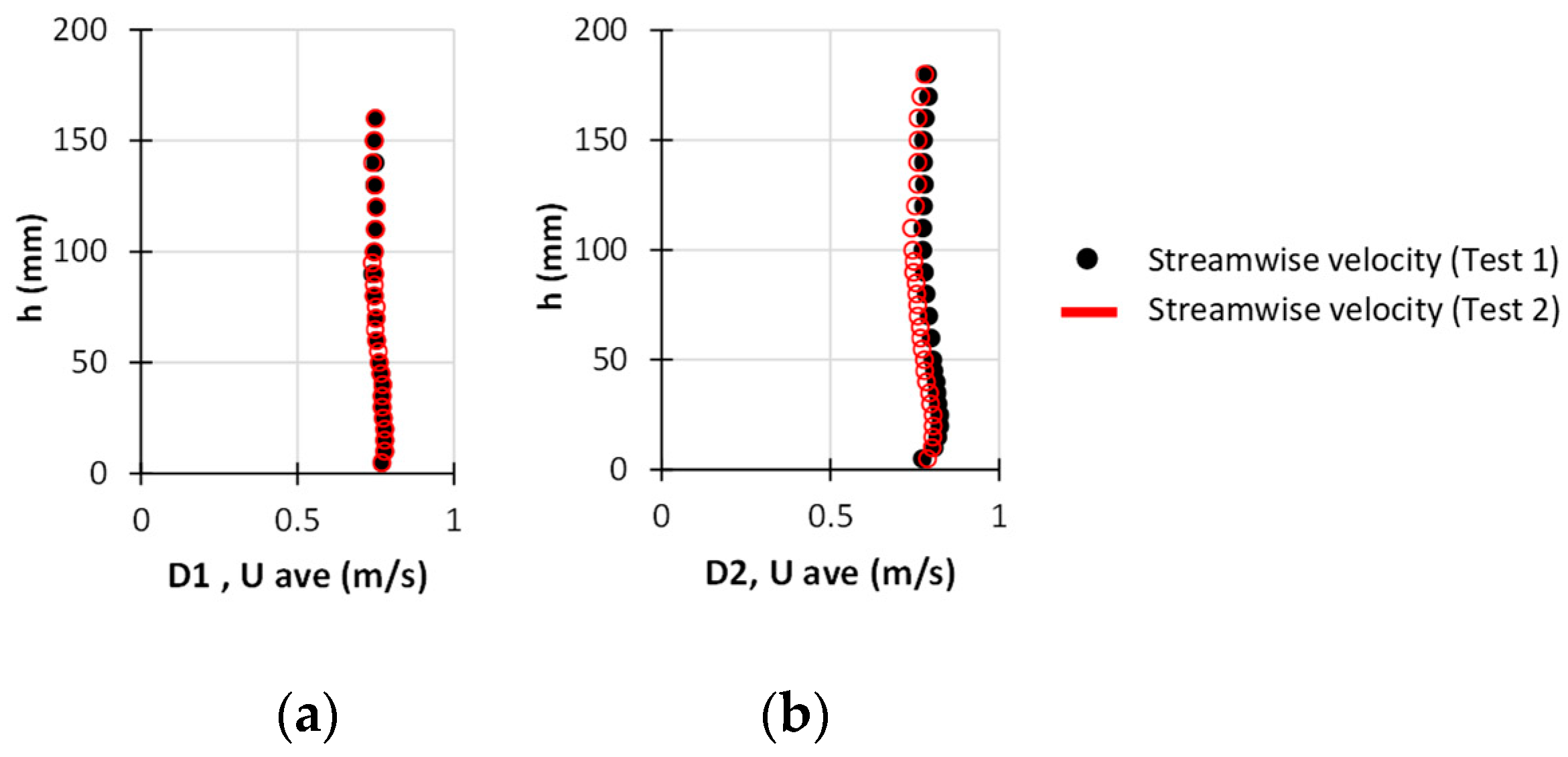
4.1. Validation Process

The simulation results closely align with the experimental measurements, particularly in the regions of steady flow. However, minor discrepancies were observed near the piers, likely due to the limitations of the turbulence modelling, mesh resolution constraints, and experimental uncertainties. To mitigate these discrepancies, we refined the mesh near the piers and employed an adaptive time-stepping approach, which significantly improved the accuracy while maintaining the computational efficiency. Moreover, Figure 6 illustrates the streamwise velocity profiles of the undisturbed region, demonstrating a strong agreement between the numerical and experimental results, and confirming the accuracy of the simulation before the flow interacts with the piers.

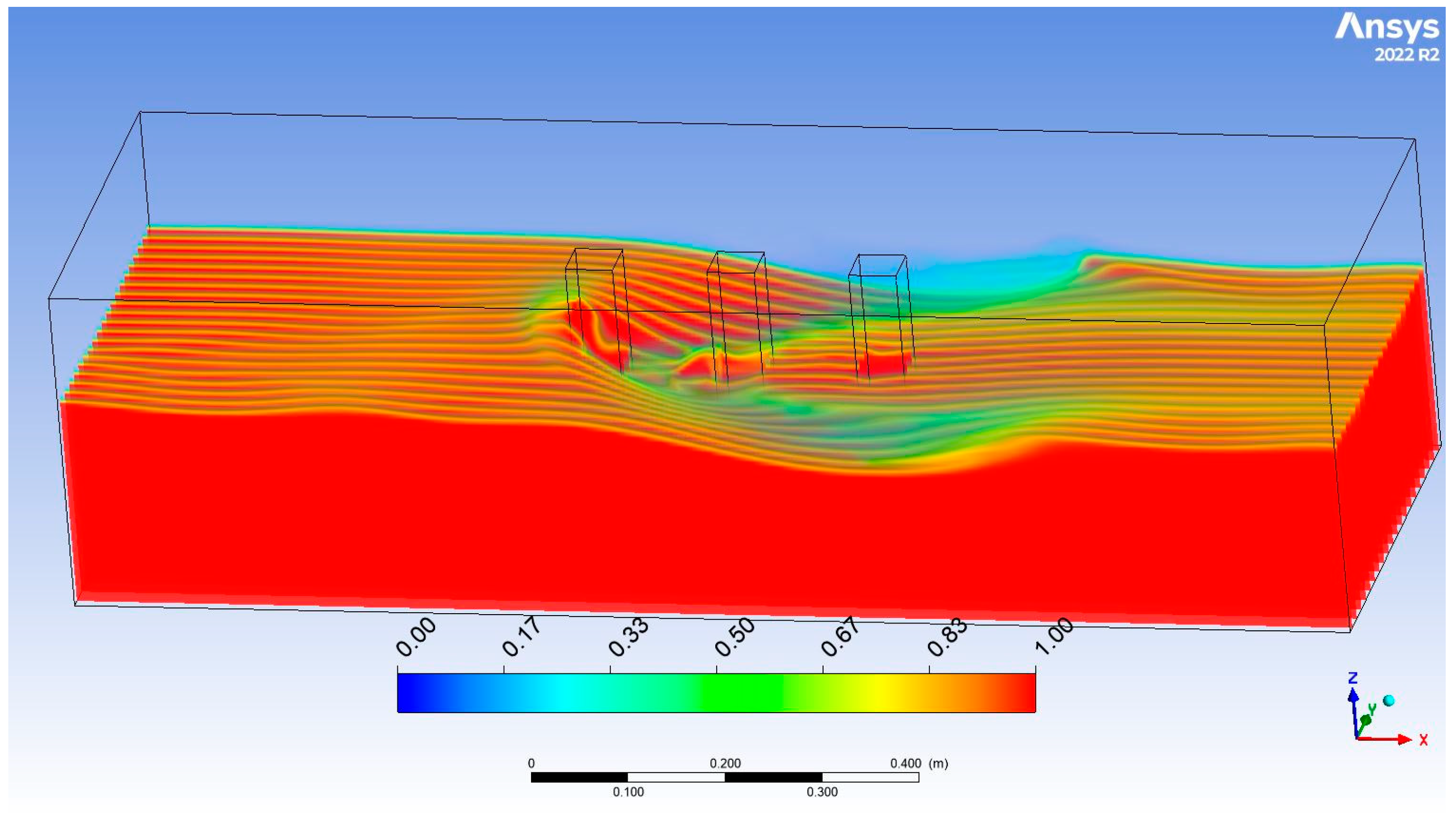
4.2. Numerical Analysis of Free-Surface Flow Around Three Tandem Piers

Figure 7, representing the water volume fraction distribution in a flow field around three tandem square piers, provides detailed insight into the complex interactions between the free-surface flow and turbulent structures, even in the absence of an experimental validation. The visualization, generated using a numerical model, illustrates the spatial distribution of the water and air phases, particularly focusing on the free-surface deformation caused by the pier-induced disturbances. The wireframe contours clearly depict the regions of flow separation and recirculation behind the piers, which are key contributors to turbulent TKE generation. The high-gradient zones in the volume fraction indicate the areas where the free surface interacts with the vortex structures, leading to energy dissipation and mixing, a critical aspect of flow turbulence.

The upstream flow is relatively uniform, as indicated by the smooth contours, but as the flow encounters the first pier, separation occurs, generating wake regions downstream. These wake regions intensify near the second and third piers due to the cumulative effects of vortex shedding and turbulence interaction between the piers. This phenomenon reflects the influence of the pier configuration on the redistribution of the TKE. The deformation of the free surface, particularly near the second pier, is a strong indicator of vortex-induced turbulence, which may be underestimated by the k-ε model due to its inherent assumptions about isotropic turbulence.

In addition, the colour gradient, transitioning from red (indicating the water phase) to blue (air phase), highlights the extent of the free-surface fluctuation and mixing. This detail is crucial for understanding the energy dissipation mechanisms, as the zones of strong fluctuation correspond to the areas where turbulence and TKE dominate. By observing these regions, one can infer the efficiency of the numerical model at capturing the interaction between the flow structures and the free surface.

Figure 8 also presents the water volume fraction contours, but for specific planes $(z=30,z=85,\mathrm{a}\mathrm{n}\mathrm{d}z=130)$ in the flow domain, showing the interaction between the flow field and the three tandem square piers. The contours provide a detailed view of the free-surface behaviour and vortex formation at different depths, emphasizing the dynamic turbulence characteristics in the vicinity of the piers.

The flow around the first pier generates strong wake regions, as seen in the high-gradient contours at $z=30$ and $z=85$. These regions exhibit substantial energy dissipation and vortex shedding, which significantly influence the downstream flow behaviour. The wake structures become more organized and elongated downstream of the second and third piers, reflecting the stabilizing effects of flow reattachment and reduced turbulence intensity. At $z=130$, the flow shows more developed and uniform patterns with reduced vortex intensity, highlighting the gradual dissipation of the TKE as the flow moves downstream.

When compared to the findings of Ikani and Pu [14], who analyzed similar flow scenarios using both computational and experimental methods, the results align well in terms of the overall flow velocity and vortex formation patterns. Ikani and Pu [40]’s work demonstrated that the primary vortices formed behind the piers dominate the flow field, with their strength diminishing in the downstream region. However, Figure 8 highlights a more pronounced underestimation of the vortex strength and TKE, likely due to the limitations of the k-$\epsilon$ turbulence model at capturing the anisotropic turbulence and free-surface interactions. Also, the zero water fraction at the centre of the vortex, as shown in Figure 8, results from air entrainment and the free-surface deformation effects captured by the numerical model. Intense vortices generate localized pressure drops, causing surface depressions and intermittent air entrainment. This leads to regions with no water fraction, where the model predicts air entrainment or surface depression in the vortex core (studies by [39,40] support these observations). Ikani and Pu [14] utilized experimental data to validate their computational model, confirming that turbulence models like the k-$\epsilon$ struggle to accurately resolve the fine-scale vortical structures in regions of high turbulence intensity, particularly near the free surface.

The reference axes in Figure 7, Figure 8 and Figure 9 may appear different due to the intentional adjustments to the viewing angles, which were designed to enhance the visualization of the key flow characteristics, including the vortex formation, velocity distribution, and wake dynamics around the piers. These modifications to the visualization do not impact the validity of the results, as all the figures are derived from the same computational framework and accurately represent the underlying flow phenomena.

4.3. Turbulent Kinetic Energy (TKE) Distribution

The TKE distributions at planes $z=30\mathrm{m}\mathrm{m}$, $z=85\mathrm{m}\mathrm{m}$, and $z=130\mathrm{m}\mathrm{m}$, as shown in Figure 9a and Figure 9b respectively, demonstrate a detailed evaluation of the turbulence and energy transfer around the three tandem square piers. At $z=30\mathrm{m}\mathrm{m}$, the near-bed plane in Figure 5a, the TKE peaks at approximately $0.1{\mathrm{m}}^2/{\mathrm{s}}^2$ behind the first pier due to the strong vortex shedding and bed-induced shear stress. These high-energy zones diminish downstream as the wake turbulence interacts with the second and third piers, stabilizing at $0.03–0.05{\mathrm{m}}^2/{\mathrm{s}}^2$. Compared to the experimental findings of [40], which documented stronger bed-induced vortices and secondary flow effects, the $k\text{-}\epsilon$ model underestimates the TKE due to its isotropic assumptions that fail to capture the anisotropic turbulence near the bed. At $z=85\mathrm{m}\mathrm{m}$, the mid-height plane in Figure 9b, the TKE distributions show complex interactions between the primary wake vortices, with peak values of approximately $0.08{\mathrm{m}}^2/{\mathrm{s}}^2$ behind the first pier. The energy transfer between the vortices results in localized TKE increases behind the second pier, while further downstream the turbulence dissipates, stabilizing around $0.03{\mathrm{m}}^2/{\mathrm{s}}^2$. Although the numerical results align with the general vortex-driven turbulence patterns observed by [40], the $k\text{-}\epsilon$ model fails to resolve the energy redistribution associated with asymmetric vortex pairing, as observed in their experiments. At $z=130\mathrm{m}\mathrm{m}$, the energy dissipation becomes more pronounced in this plane due to the surface interactions, with the TKE values dropping below $0.01{\mathrm{m}}^2/{\mathrm{s}}^2$ by the third pier, indicating a minimal energy transfer. While the model predicts the general dissipation trend, it underrepresents the small-scale turbulence near the surface compared to Ikani et al.’s experimental observations, which documented localized shear layers and energy fluctuations. This layered, plane-by-plane comparison with the experimental results suggests a more spatially resolved assessment of the k-ε model’s performance than previously reported. In particular, this study identifies the critical flow depths, such as the near-bed and mid-depth regions, where vortex shedding and asymmetric interactions lead to a substantial underestimation of the TKE, showing the model’s limitations for resolving anisotropic turbulence features. Across all the planes, the energy transfer mechanisms reveal the limitations of the $k\text{-}\epsilon$ model for accurately resolving the TKE in regions of strong shear and wake interactions, as it systematically underestimates the turbulence magnitudes due to its isotropic framework.

At $z/h=0.4$ (downstream of the second pier), the experimental peak TKE is $0.12{\mathrm{m}}^2/{\mathrm{s}}^2,$ whereas the k-$\epsilon$ model predicts $0.09{\mathrm{m}}^2/{\mathrm{s}}^2$ (a $25\%$ underestimation). At $z/h=0.62$ (near the first pier), the experimental TKE is $0.15{\mathrm{m}}^2/{\mathrm{s}}^2$, compared to the simulated value of $0.11{\mathrm{m}}^2/{\mathrm{s}}^2(a27\%$ difference). The mean absolute percentage error (MAPE) for the TKE predictions across all measurement locations is 22.5%. The largest local error occurs at $z/h$ = 0.62, where the TKE is underestimated by 27%. The smallest error occurs at $z/h$ = 0.15, where the TKE underestimation is below 10%. While these errors reflect the dissipation bias of the standard k-$\epsilon$ model, the qualitative agreement with the experimental turbulence structures remains strong.

An essential parameter for quantifying the flow turbulence is the TKE, which is derived from the mean values of the turbulent eddies. Hence, it can be estimated using Equation (13) as follows [67,68,69]:

$$TKE=0.5(\overline{u^{{\prime }^2}}+\overline{v^{{\prime }^2}}+\overline{w^{{\prime }^2}})$$

(13)

Figure 10 shows the TKE plots at locations after each pier. As a result, the analysis from the distribution shows that the TKE is relatively smaller at upstream undisturbed locations throughout the flow depth. In comparison, its values in the flow wake region are significantly altered due to the higher velocity fluctuations caused by enhanced turbulence mixing. The TKE is increased due to the flow separation caused by the piers and the formation of the wake region. The TKE attains its peak at the near bed and is increased at the side of first pier. It is estimated that the highest TKE value occurs near the second pier (i.e., the middle of whole piers’ vicinity). As an individual point, the TKE value is highest at $z/h=0.4$ after the second pier, and at $z/h=0.62$ behind the first pier. Based on the simulation, there are discrepancies between the model’s predictions and the experimental data, where the simulation clearly underestimates the measurement due to the estimation of the $k\text{-}\epsilon$ model that dissipates the energy disproportionately. However, there is a consistent trend observed in the simulated TKE when benchmarked by the experimental data. Furthermore, there is a satisfactory agreement of the simulated locations of the TKE peak when compared to each vortex-governed measured point. Conclusively, even though the employed k-ε model does not produce the TKE magnitude with good accuracy, it is a very practical model and permits fast computation without needing to consider large- or small-scale physical eddies. Additionally, with its ability to capture the right key characteristic locations and features of the TKE distribution, the k-ε model should be considered as an optimum model with which to represent flow turbulence in piers-induced flows. From both the simulations and measurements, near the flow surface the value of the TKE becomes very small due to the damping of the velocity fluctuations.

5. Conclusions

This study evaluated the performance of the k-ε turbulence model for predicting the Turbulent Kinetic Energy (TKE) distributions around a group of three tandem piers using numerical simulations and experimental measurements. The numerical model, implemented in ANSYS FLUENT with the VOF approach, was validated against laboratory measurements obtained via ADV. A comparison revealed that the k-ε model systematically underestimated the TKE, particularly in highly turbulent regions influenced by a vortex-induced flow. The highest local discrepancy occurred at z/h = 0.62, near the first pier, where the model underestimated the TKE by 27%. At z/h = 0.4, downstream of the second pier, the peak experimental TKE was 0.12 ${\mathrm{m}}^2/{\mathrm{s}}^2$, while the model predicted 0.09 m²/s², corresponding to a 25% underestimation. The lowest discrepancy was observed at z/h = 0.15, where the underestimation remained below 10%. These results highlight the limitations of the k-ε model for accurately capturing the turbulence intensity in vortex-dominated regions, primarily due to its isotropic turbulence assumption. Despite these discrepancies, the model effectively captured the overall TKE distribution trend, making it suitable for large-scale flow predictions while acknowledging its reduced accuracy for resolving small-scale turbulence structures. This study also presented a detailed, zone-specific evaluation of the k-ε model’s performance regarding structure-induced turbulence, revealing its critical underestimations of the TKE in vortex-dominated flow regions. The findings show a novel perspective of the model’s spatial limitations and serve as a practical reference for selecting the appropriate turbulence models for large-scale hydraulic simulations, where both accuracy and computational efficiency are required.

References

1. Ali, K.H.; Karim, O. Simulation of flow around piers. J. Hydraul. Res. 2002, 40, 161–174. [Google Scholar]
2. Dey, S.; Barbhuiya, A.K. 3D flow field in a scour hole at a wing-wall abutment. J. Hydraul. Res. 2006, 44, 33–50. [Google Scholar]
3. Mutlu Sumer, B. Mathematical modelling of scour: A review. J. Hydraul. Res. 2007, 45, 723–735. [Google Scholar] [CrossRef]
4. Kocaman, S. Prediction of backwater profiles due to bridges in a compound channel using CFD. Adv. Mech. Eng. 2014, 6, 905217. [Google Scholar]
5. Soori, S.; Karami, H. Laboratory study on relative energy loss and backwater rise at bridge piers and abutment. Model. Earth Syst. Environ. 2024, 10, 1359–1373. [Google Scholar]
6. Pagliara, S.; Carnacina, I. Temporal scour evolution at bridge piers: Effect of wood debris roughness and porosity. J. Hydraul. Res. 2010, 48, 3–13. [Google Scholar]
7. Soori, S.; Babaali, H.; Soori, N. An optimal design of the inlet and outlet obstacles at USBR II Stilling Basin. Int. J. Sci. Eng. Appl. 2017, 6, 134–142. [Google Scholar]
8. Bressan, F.; Ballio, F.; Armenio, V. Turbulence around a scoured bridge abutment. J. Turbul. 2011, 12, N3. [Google Scholar] [CrossRef]
9. Rodi, W.; Constantinescu, G.; Stoesser, T. Large-Eddy Simulation in Hydraulics; CRC Press: Boca Raton, FL, USA, 2013. [Google Scholar]
10. Keylock, C.; Constantinescu, G.; Hardy, R. The application of computational fluid dynamics to natural river channels: Eddy resolving versus mean flow approaches. Geomorphology 2012, 179, 1–20. [Google Scholar] [CrossRef]
11. Kara, S.; Kara, M.C.; Stoesser, T.; Sturm, T.W. Free-surface versus rigid-lid LES computations for bridge-abutment flow. J. Hydraul. Eng. 2015, 141, 04015019. [Google Scholar]
12. Al-Jubouri, M.; Ray, R.P.; Abbas, E.H. Advanced numerical simulation of scour around bridge piers: Effects of pier geometry and debris on scour depth. J. Mar. Sci. Eng. 2024, 12, 1637. [Google Scholar] [CrossRef]
13. Alvarez, L.V.; Grams, P.E. An Eddy-Resolving Numerical Model to Study Turbulent Flow, Sediment, and Bed Evolution Using Detached Eddy Simulation in a Lateral Separation Zone at the Field-Scale. J. Geophys. Res. Earth Surf. 2021, 126, e2021JF006149. [Google Scholar] [CrossRef]
14. Ikani, N.; Pu, J.H.; Hanmaiahgari, P.R.; Kumar, B.; Al-Qadami, E.H.H.; Razi, M.A.M.; Zang, S.-Y. Computational and experimental analysis of flow velocity and complex vortex formation around a group of bridge piers. Water Sci. Eng. 2025; in press. [Google Scholar] [CrossRef]
15. Huang, W.; Yang, Q.; Xiao, H. CFD modeling of scale effects on turbulence flow and scour around bridge piers. Comput. Fluids 2009, 38, 1050–1058. [Google Scholar] [CrossRef]
16. Chatterjee, D.; Mazumder, B.S.; Ghosh, S.; Debnath, K. Turbulent flow characteristics over forward-facing obstacle. J. Turbul. 2021, 22, 141–179. [Google Scholar] [CrossRef]
17. Uchida, T.; Ato, T.; Kobayashi, D.; Maghrebi, M.F.; Kawahara, Y. Hydrodynamic forces on emergent cylinders in non-uniform flow. Environ. Fluid Mech. 2022, 22, 1355–1379. [Google Scholar] [CrossRef]
18. Roulund, A.; Sumer, B.M.; Fredsøe, J.; Michelsen, J. Numerical and experimental investigation of flow and scour around a circular pile. J. Fluid Mech. 2005, 534, 351–401. [Google Scholar] [CrossRef]
19. Ghzayel, A.; Beaudoin, A. Three-dimensional numerical study of a local scour downstream of a submerged sluice gate using two hydro-morphodynamic models, SedFoam and FLOW-3D. Comptes Rendus Mécanique 2023, 351, 525–550. [Google Scholar] [CrossRef]
20. Lai, Y.G.; Liu, X.; Bombardelli, F.A.; Song, Y. Three-dimensional numerical modeling of local scour: A state-of-the-art review and perspective. J. Hydraul. Eng. 2022, 148, 03122002. [Google Scholar] [CrossRef]
21. Calixto, N.C.; Zambrano, M.C.; Castaño, A.G.; Soto, G.C. Analysis of a three-dimensional numerical modeling approach for predicting scour processes in longitudinal walls of granular bedding rivers. EUREKA Phys. Eng. 2023, 4, 168–179. [Google Scholar] [CrossRef]
22. Khosronejad, A.; Kang, S.; Sotiropoulos, F. Experimental and computational investigation of local scour around bridge piers. Adv. Water Resour. 2012, 37, 73–85. [Google Scholar] [CrossRef]
23. Chatelain, M.; Proust, S. Open-channel flows through emergent rigid vegetation: Effects of bed roughness and shallowness on the flow structure and surface waves. Phys. Fluids 2021, 33, 106602. [Google Scholar] [CrossRef]
24. Unger, J.; Hager, W.H. Down-flow and horseshoe vortex characteristics of sediment embedded bridge piers. Exp. Fluids 2007, 42, 1–19. [Google Scholar] [CrossRef]
25. Sahin, B.; Ozturk, N.A. Behaviour of flow at the junction of cylinder and base plate in deep water. Measurement 2009, 42, 225–240. [Google Scholar] [CrossRef]
26. Sahin, B.; Akilli, H.; Karakus, C.; Akar, M.; Ozkul, E. Qualitative and quantitative measurements of horseshoe vortex formation in the junction of horizontal and vertical plates. Measurement 2010, 43, 245–254. [Google Scholar] [CrossRef]
27. Zhao, M.; Cheng, L.; Zang, Z. Experimental and numerical investigation of local scour around a submerged vertical circular cylinder in steady currents. Coast. Eng. 2010, 57, 709–721. [Google Scholar] [CrossRef]
28. Ettema, R.; Kirkil, G.; Muste, M. Similitude of large-scale turbulence in experiments on local scour at cylinders. J. Hydraul. Eng. 2006, 132, 33–40. [Google Scholar] [CrossRef]
29. Cheng, Z.; Koken, M.; Constantinescu, G. Approximate methodology to account for effects of coherent structures on sediment entrainment in RANS simulations with a movable bed and applications to pier scour. Adv. Water Resour. 2018, 120, 65–82. [Google Scholar] [CrossRef]
30. Sinha, S.K.; Sotiropoulos, F.; Odgaard, A.J. Three-dimensional numerical model for flow through natural rivers. J. Hydraul. Eng. 1998, 124, 13–24. [Google Scholar] [CrossRef]
31. Dargahi, B. Controlling mechanism of local scouring. J. Hydraul. Eng. 1990, 116, 1197–1214. [Google Scholar] [CrossRef]
32. Xiong, W.; Cai, C.S.; Kong, B.; Kong, X. CFD simulations and analyses for bridge-scour development using a dynamic-mesh updating technique. J. Comput. Civ. Eng. 2016, 30, 04014121. [Google Scholar]
33. Guemou, B.; Seddini, A.; Ghenim, A.N. Numerical investigations of the round-nosed bridge pier length effects on the bed shear stress. Prog. Comput. Fluid Dyn. Int. J. 2016, 16, 313–321. [Google Scholar]
34. Soori, S.; Hajikandi, H. Numerical Computation of Flow Reattachment Lengthovera Backward-Facing Step at High Reynolds Number. Int. J. Res. Eng. 2017, 4, 145–149. [Google Scholar]
35. Svsndl, P.; Suresh, K. Simulation of flow behavior around bridge piers using ANSYS–CFD. Int. J. Eng. Sci. Invent. (IJESI) 2018, 7, 13–22. [Google Scholar]
36. Lahsaei, K.; Vaghefi, M.; Sedighi, F.; Chooplou, C.A. Numerical simulation of flow pattern at a divergent pier in a bend with different relative curvature radii using ansys fluent. Eng. Rev. 2022, 42, 63–85. [Google Scholar]
37. Ahmed, A.A.; Ismael, A.A. Comparing the 3D Flow Behavior Around Different Bridge Pier Shapes Using CFD-Fluent: Implications for Reducing Local Scour. Math. Model. Eng. Probl. 2024, 11, 1315–1322. [Google Scholar]
38. Mueller, D.S.; Abad, J.D.; García, C.M.; Gartner, J.W.; García, M.H.; Oberg, K.A. Errors in acoustic Doppler profiler velocity measurements caused by flow disturbance. J. Hydraul. Eng. 2007, 133, 1411–1420. [Google Scholar]
39. Ikani, N.; Pu, J.H.; Taha, T.; Hanmaiahgarib, P.R.; Penna, N. Bursting phenomenon created by bridge piers group in open channel flow. Environ. Fluid Mech. 2023, 23, 125–140. [Google Scholar]
40. Ikani, N.; Pu, J.H.; Zang, S.; Al-Qadami, E.H.H.; Razi, A. Detailed turbulent structures investigation around piers group induced flow. Exp. Therm. Fluid Sci. 2024, 152, 111112. [Google Scholar]
41. Chanson, H.; Leng, X. Acoustic Doppler Velocimetry in Transient Free-Surface Flows: Field and Laboratory Experience with Bores and Surges. J. Hydraul. Eng. 2024, 150, 04024034. [Google Scholar]
42. Roache, P. Verification and Validation in Computational Science and Engineering; Hermosa Publishers: Hermosa Beach, CA, USA, 1998. [Google Scholar]
43. Babuska, I.; Oden, J.T. Verification and validation in computational engineering and science: Basic concepts. Comput. Methods Appl. Mech. Eng. 2004, 193, 4057–4066. [Google Scholar] [CrossRef]
44. Oberkampf, W.L.; Trucano, T.G. Verification and validation in computational fluid dynamics. Prog. Aerosp. Sci. 2002, 38, 209–272. [Google Scholar]
45. Mojtahedi, A.; Soori, N.; Mohammadian, M. Energy dissipation evaluation for stepped spillway using a fuzzy inference system. SN Appl. Sci. 2020, 2, 1466. [Google Scholar]
46. Tu, J.; Yeoh, G.H.; Liu, C.; Tao, Y. Computational Fluid Dynamics: A Practical Approach; Elsevier: Amsterdam, The Netherlands, 2023. [Google Scholar]
47. Oveici, E.; Tayari, O.; Jalalkamali, N. Experimental (ADV & PIV) and numerical (CFD) comparisons of 3D flow pattern around intact and damaged bridge piers. Pertanika J. Sci. Technol. 2020, 28, 523–544. [Google Scholar]
48. Abad, J.D.; Musalem, R.A.; García, C.M.; Cantero, M.I.; García, M.H. Exploratory study of the influence of the wake produced by acoustic Doppler velocimeter probes on the water velocities within measurement volume. Crit. Transit. Water Environ. Resour. Manag. 2004, 1–9. [Google Scholar] [CrossRef]
49. Sarkardeh, H.; Zarrati, A.R.; Jabbari, E.; Marosi, M. Numerical simulation and analysis of flow in a reservoir in the presence of vortex. Eng. Appl. Comput. Fluid Mech. 2014, 8, 598–608. [Google Scholar]
50. Quaresma, A.; Pinheiro, A.N. Analysis of flows in pool-type fishways using acoustic Doppler velocimetry (ADV) and computational fluid dynamics (CFD). In Proceedings of the 10th International Symposium on Ecohydraulics, Trodheim, Norway, 23–27 June 2014. [Google Scholar]
51. Shaheed, R.; Mohammadian, A.; Gildeh, H.K. A comparison of standard k–ε and realizable k–ε turbulence models in curved and confluent channels. Environ. Fluid Mech. 2019, 19, 543–568. [Google Scholar] [CrossRef]
52. Rodi, W. Turbulence modeling and simulation in hydraulics: A historical review. J. Hydraul. Eng. 2017, 143, 03117001. [Google Scholar] [CrossRef]
53. Pu, J.H.; Hussain, K.; Tait, S.J. Simulation of turbulent free surface obstructed flow within channels. In Proceedings of the 32nd IAHR World Congress, Venice, Italy, 1–6 July 2007. [Google Scholar]
54. Pu, J.H.; Cheng, N.-S.; Tan, S.K.; Shao, S. Source term treatment of SWEs using surface gradient upwind method. J. Hydraul. Res. 2012, 50, 145–153. [Google Scholar]
55. Pu, J.H.; Shao, S.; Huang, Y. Numerical and experimental turbulence studies on shallow open channel flows. J. Hydro Environ. Res. 2014, 8, 9–19. [Google Scholar]
56. Argyropoulos, C.D.; Markatos, N. Recent advances on the numerical modelling of turbulent flows. Appl. Math. Model. 2015, 39, 693–732. [Google Scholar]
57. Rodi, W. Turbulence Models and Their Application in Hydraulics; Routledge: Oxford, UK, 2017. [Google Scholar]
58. Graf, W.; Istiarto, I. Flow pattern in the scour hole around a cylinder. J. Hydraul. Res. 2002, 40, 13–20. [Google Scholar] [CrossRef]
59. Pu, J.H. Turbulence modelling of shallow water flows using Kolmogorov approach. Comput. Fluids 2015, 115, 66–74. [Google Scholar] [CrossRef]
60. Kim, S.-E.; Choudhury, D.; Patel, B. Computations of Complex Turbulent Flows Using the Commercial Code Fluent, in Modeling Complex Turbulent Flows; Springer: Berlin/Heidelberg, Germany, 1999; pp. 259–276. [Google Scholar]
61. Fluent, A. Ansys Fluent Theory Guide; Ansys Inc.: Canonsburg, PA, USA, 2011; Volume 15317, pp. 724–746. [Google Scholar]
62. Chiew, Y.-M. Mechanics of riprap failure at bridge piers. J. Hydraul. Eng. 1995, 121, 635–643. [Google Scholar] [CrossRef]
63. Discetti, S.; Coletti, F. Volumetric velocimetry for fluid flows. Meas. Sci. Technol. 2018, 29, 042001. [Google Scholar] [CrossRef]
64. Pu, J.H. Velocity profile and turbulence structure measurement corrections for sediment transport-induced water-worked bed. Fluids 2021, 6, 86. [Google Scholar] [CrossRef]
65. Franca, M.J.R.P.d. A Field Study of Turbulent Flows in Shallow Gravel-Bed Rivers; EPFL: Lausanne, Switzerland, 2005. [Google Scholar]
66. Yu, G.; Tan, S.-K. Errors in the bed shear stress as estimated from vertical velocity profile. J. Irrig. Drain. Eng. 2006, 132, 490–497. [Google Scholar] [CrossRef]
67. Khaple, S.; Hanmaiahgari, P.R.; Gaudio, R.; Dey, S. Splitter plate as a flow-altering pier scour countermeasure. Acta Geophys. 2017, 65, 957–975. [Google Scholar] [CrossRef]
68. Khan, M.A.; Sharma, N.; Pu, J.; Aamir, M.; Pandey, M. Two-dimensional turbulent burst examination and angle ratio utilization to detect scouring/sedimentation around mid-channel bar. Acta Geophys. 2021, 69, 1335–1348. [Google Scholar] [CrossRef]
69. Devi, K.; Mishra, S.; Hanmaiahgari, P.R.; Pu, J.H. Wake flow field of a wall-mounted pipe with spoiler on a rough channel bed. Acta Geophys. 2023, 71, 2865–2881. [Google Scholar] [CrossRef]
Figure 1. Mesh refinement strategy around piers (plan view).
Water 17 01100 g001aWater 17 01100 g001b
Figure 2. Refined mesh around piers (plan view).
Water 17 01100 g002
Figure 3. (a) Schematic plan of the ADV measurement locations within the experimental setup and (b) the group of three square pier placement in the open channel flume.
Water 17 01100 g003
Figure 4. ADV measuring principle and experimental setup.
Water 17 01100 g004
Figure 5. Streamwise velocity profiles in the undisturbed region for accuracy validation and experimental uncertainty assessment before flow–pier interaction.
Water 17 01100 g005
Figure 6. Comparison of the streamwise velocity profiles of the undisturbed region: (a) numerical simulation, (b) experimental measurements.
Water 17 01100 g006
Figure 7. Water volume fraction distribution around three tandem square piers.
Water 17 01100 g007
Figure 8. Water volume fraction contours at planes z = 30 , z = 85 , and z = 130   m m , extending the vortex formation and free-surface flow patterns. (The reference axes show a visual representation aligned with the simulation’s global coordinate system, where the z-axis represents the vertical direction to enhance clarity and accurately convey the spatial orientation of the presented data.).
Water 17 01100 g008
Figure 9. The TKE distributions at different planes: (a) z = 30   m m and (b) z = 85   m m . (The z-plane measurement follows the standard coordinate system, where the z-axis represents the vertical direction).
Water 17 01100 g009
Figure 10. Turbulent Kinetic Energy (TKE) logarithmic distribution of numerical and experimental tests after each pier and undisturbed zone.
Water 17 01100 g010
Disclaimer/Publisher’s Note: The statements, opinions and data contained in all publications are solely those of the individual author(s) and contributor(s) and not of MDPI and/or the editor(s). MDPI and/or the editor(s) disclaim responsibility for any injury to people or property resulting from any ideas, methods, instructions or products referred to in the content.