
Hydrological Dynamics of Raipur, Chhattisgarh in India: Surface–Groundwater Interaction Amidst Urbanization


Abstract
:1. Introduction
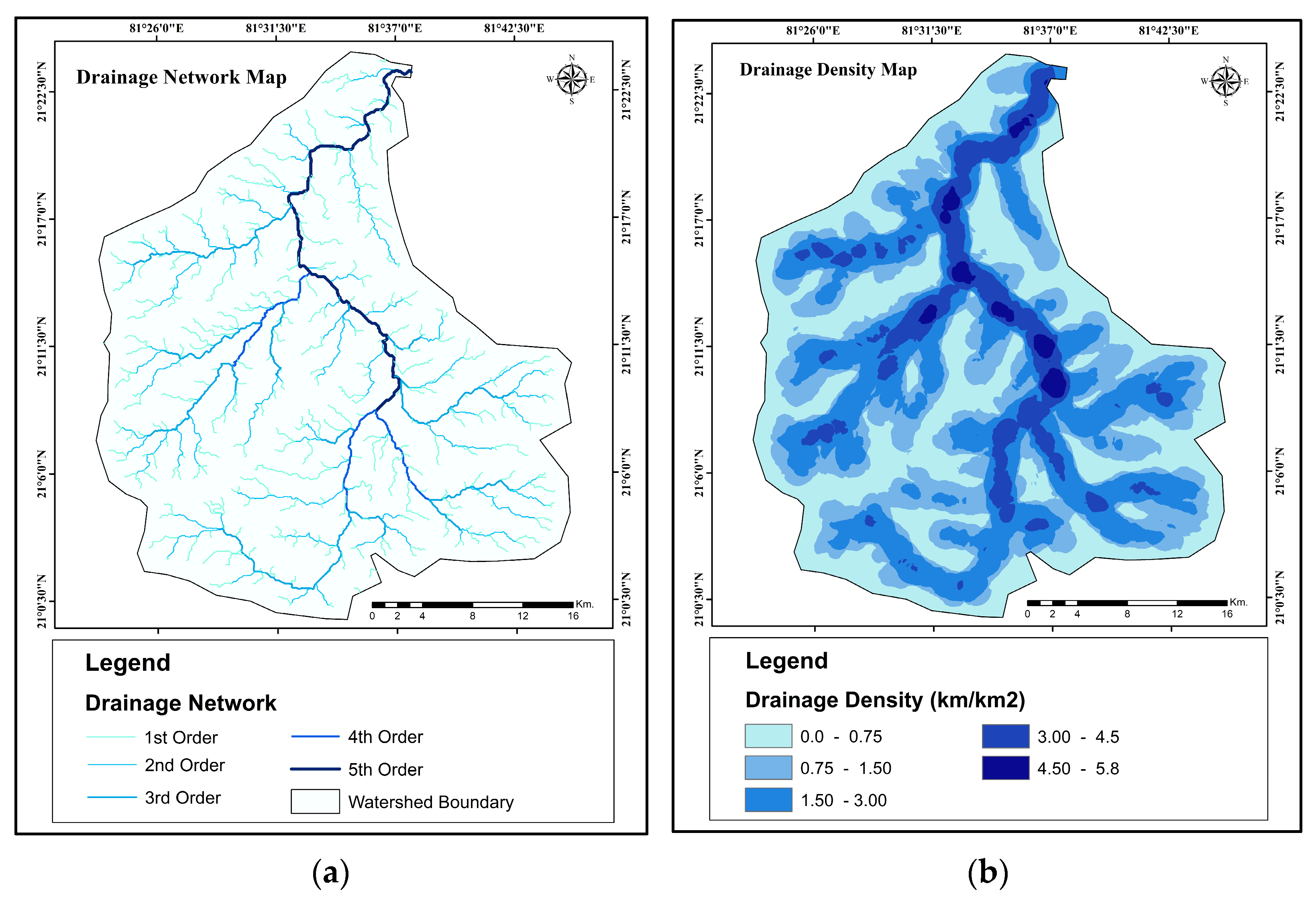
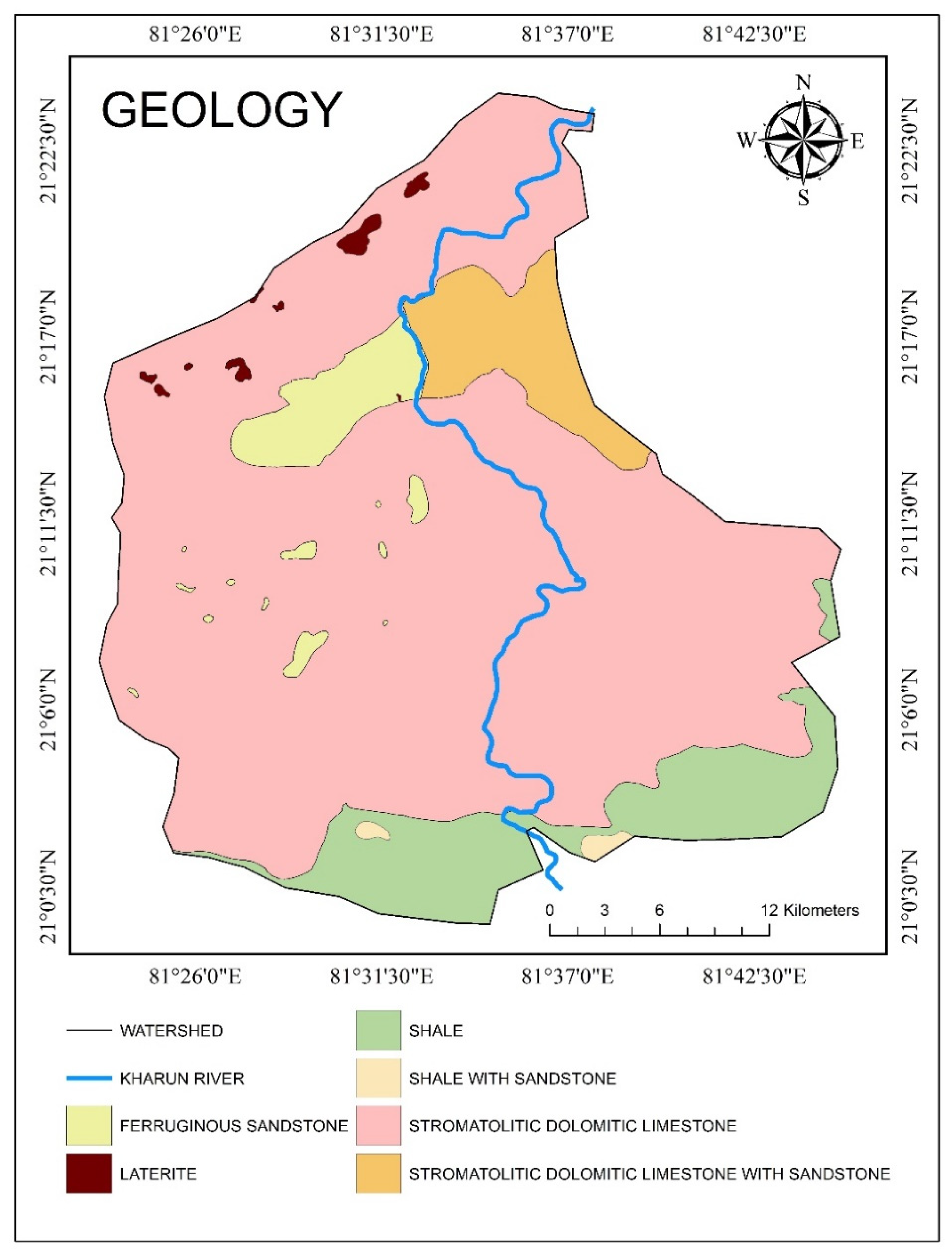
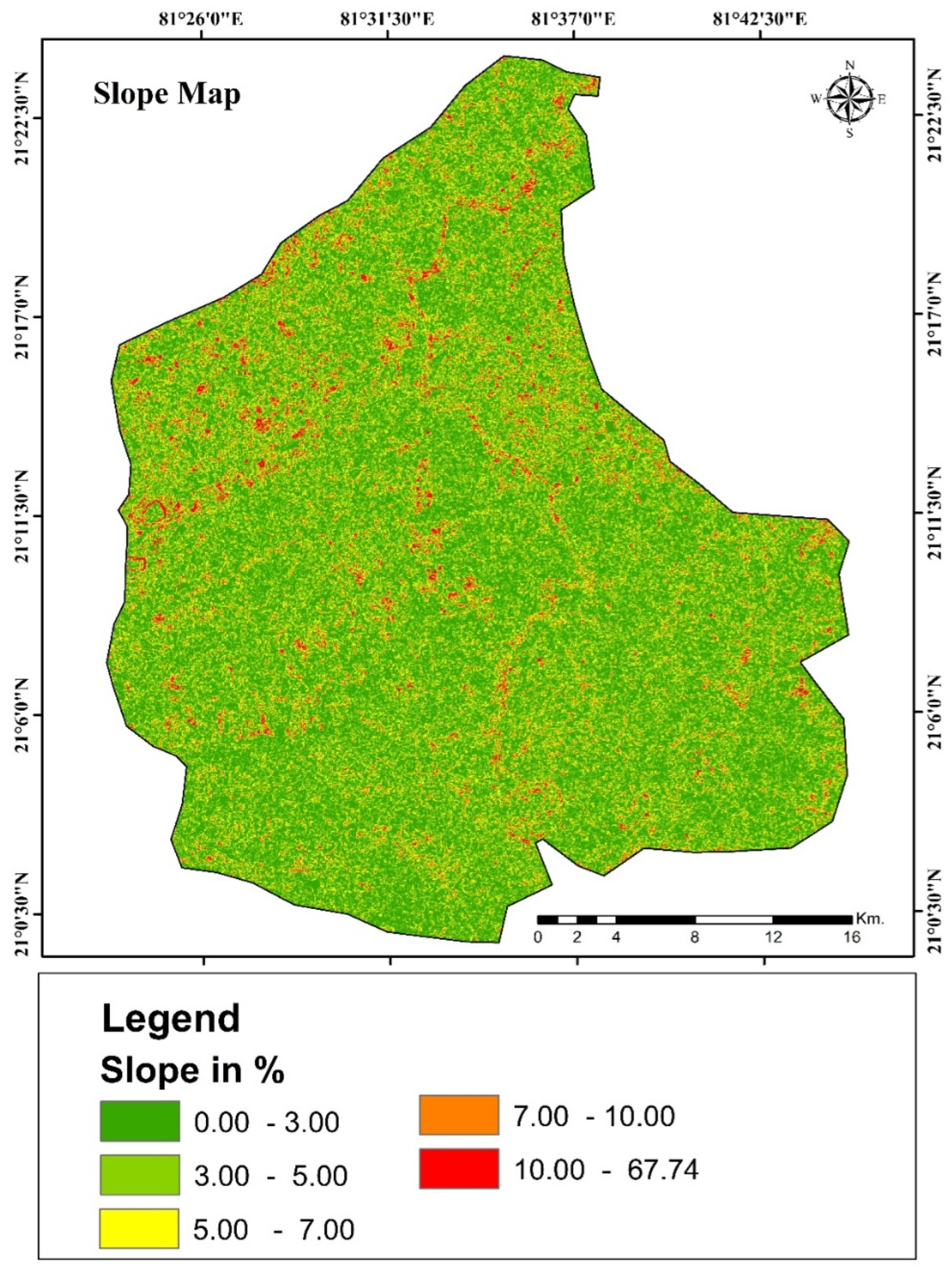
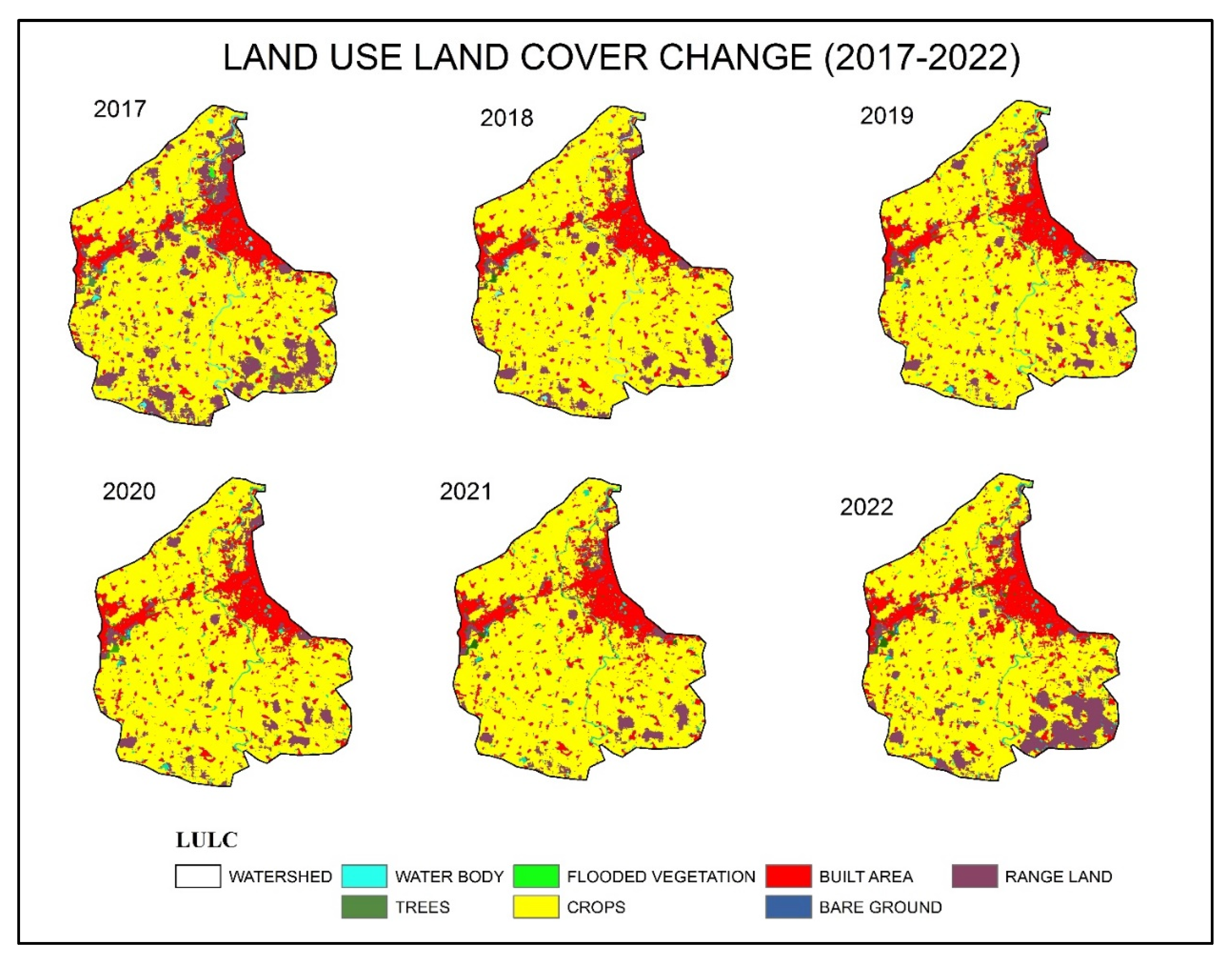
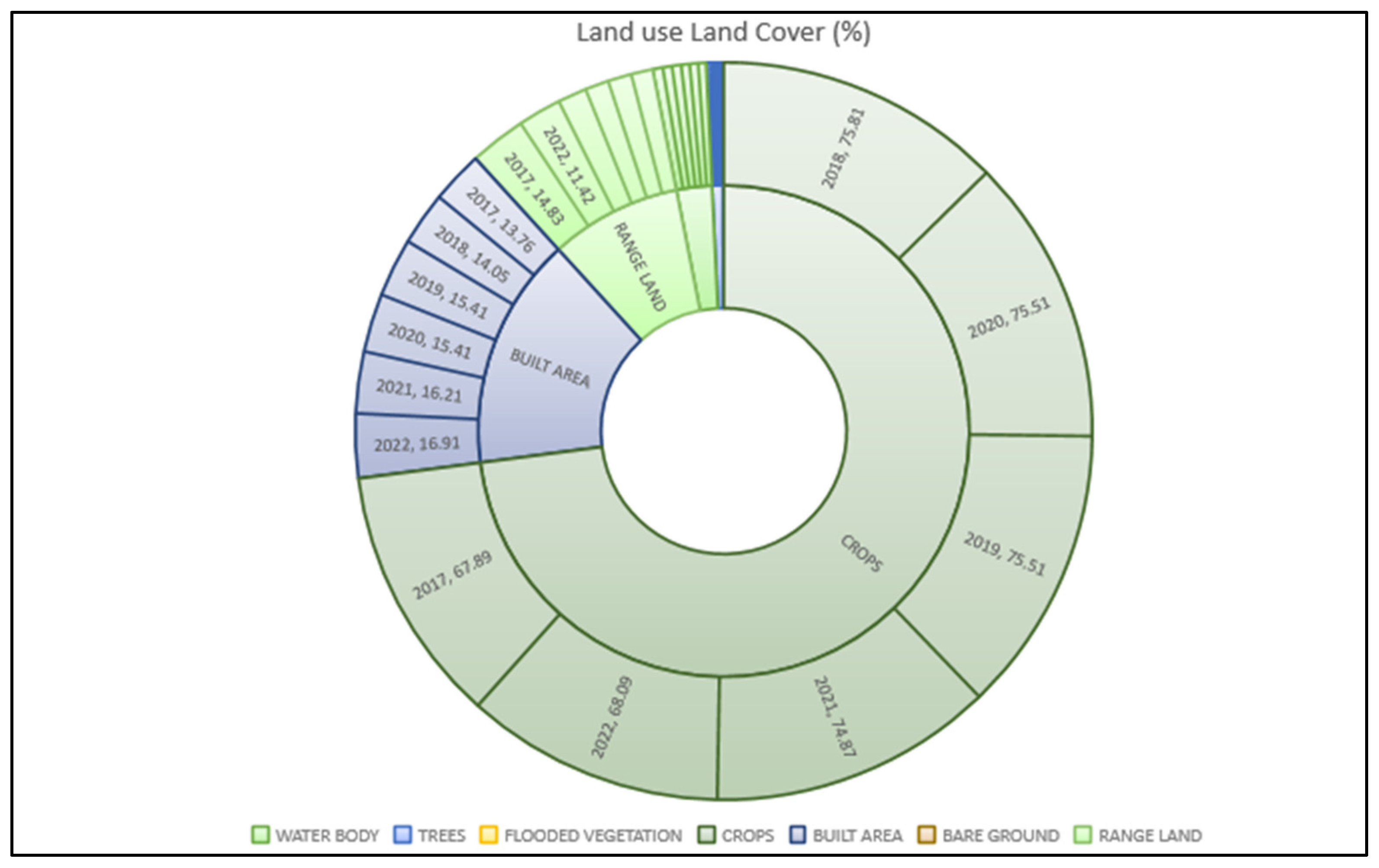
Overview of the Study Area
2. Literature Review
3. Materials and Methods
3.1. Groundwater Quality Study
3.2. Groundwater and Surface Water Assessment
3.3. Stable Isotope Analysis
4. Results and Discussion
4.1. Ground Water Table (GWT) Study
4.2. Groundwater and Surface Water Type
4.2.1. pH (Potential of Hydrogen)
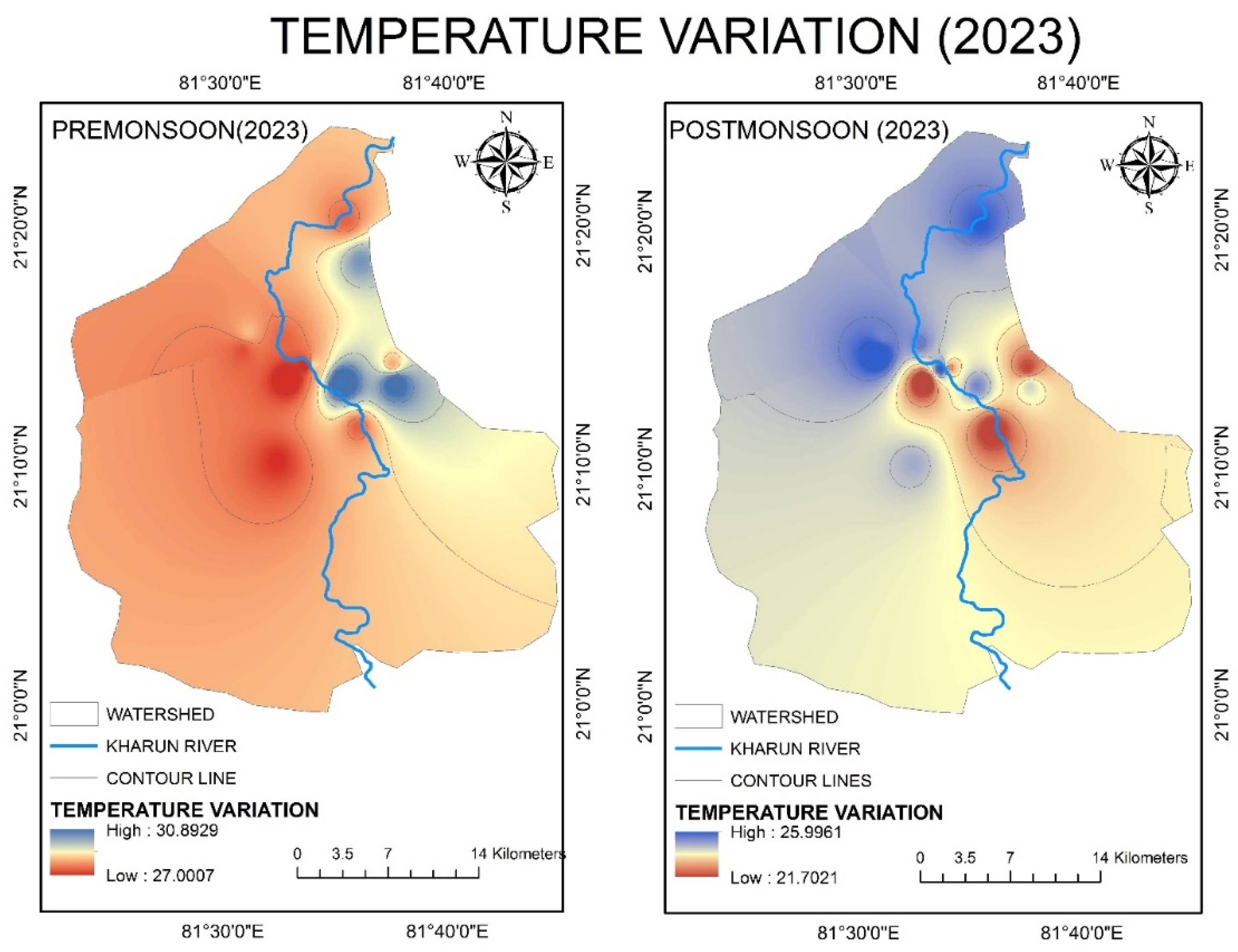
4.2.2. Temperature
4.2.3. Total Dissolved Solids (TDS)
4.2.4. Electrical Conductivity (EC)
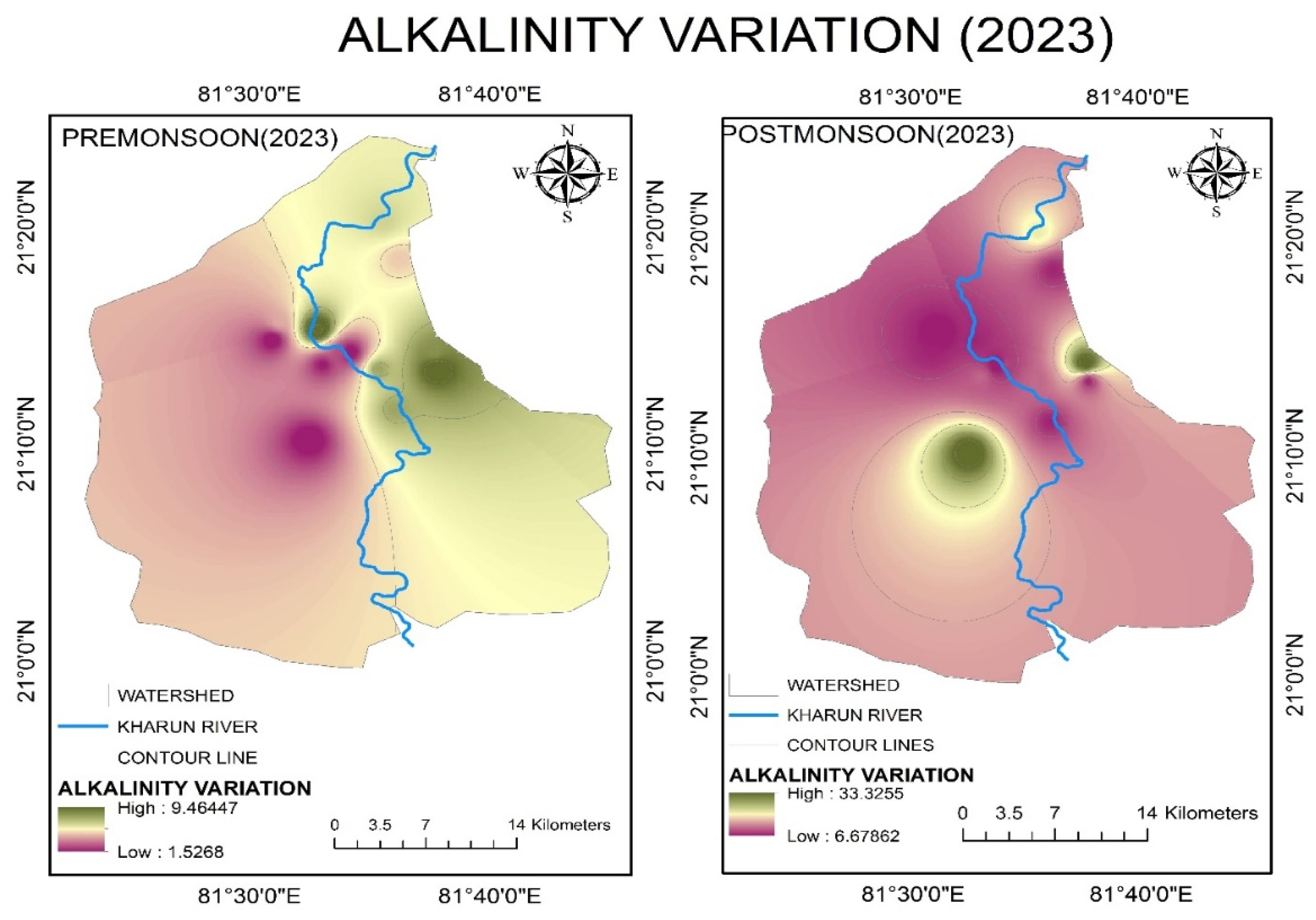
4.2.5. Alkalinity
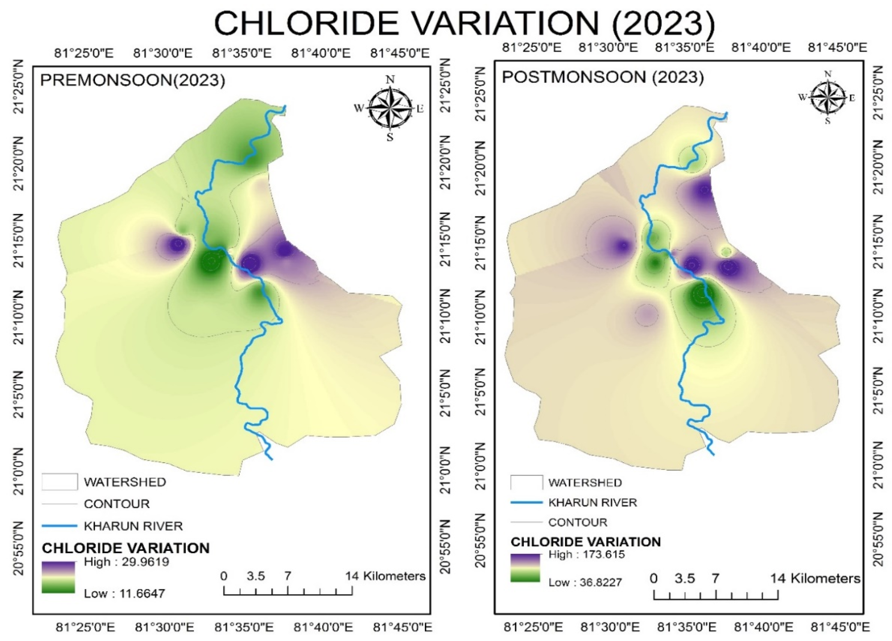
4.2.6. Chloride (Cl−)
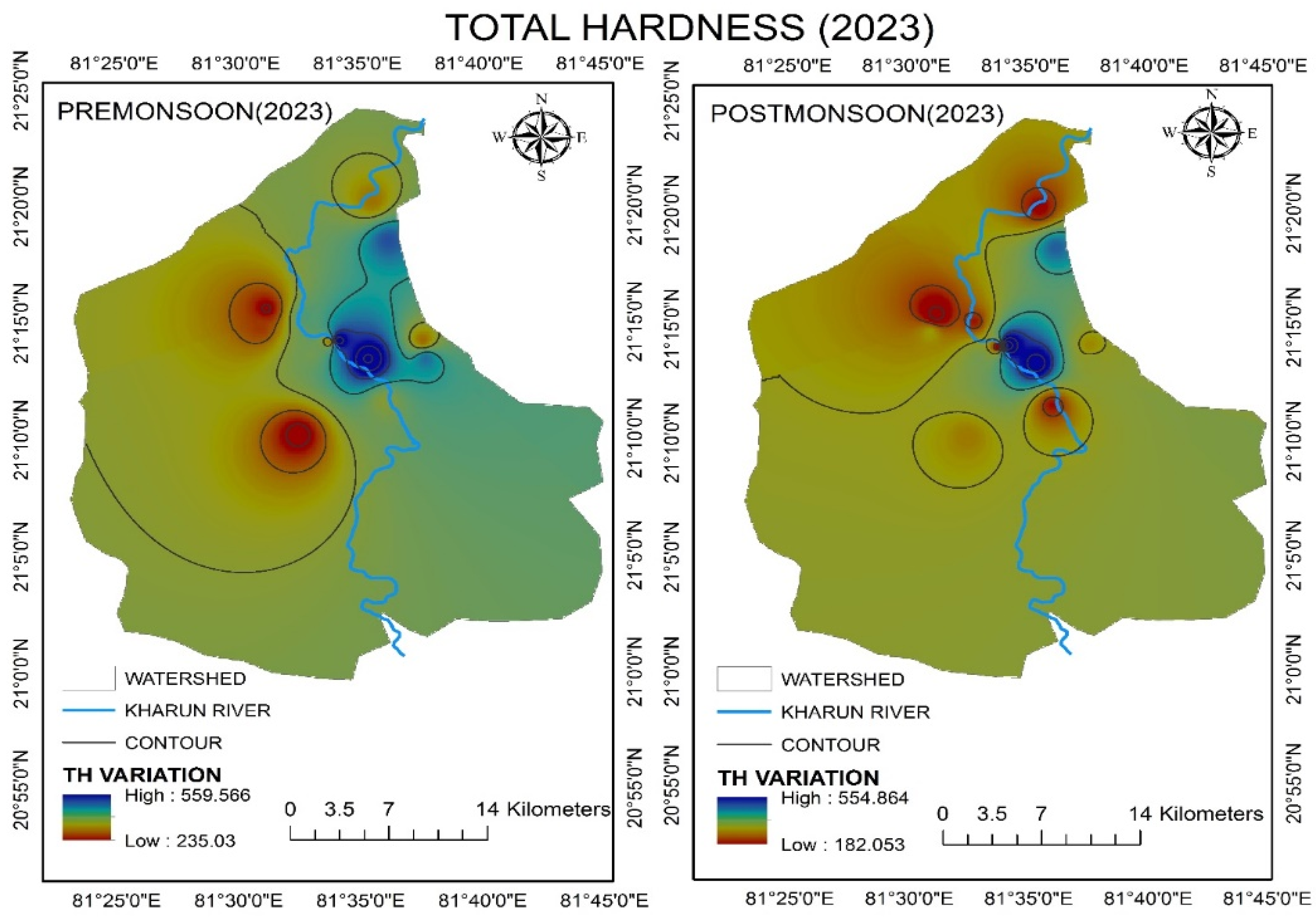
4.2.7. Total Hardness (TH)
4.2.8. Calcium (Ca2+)
4.2.9. Magnesium (Mg2+)
4.2.10. Sodium (Na+)
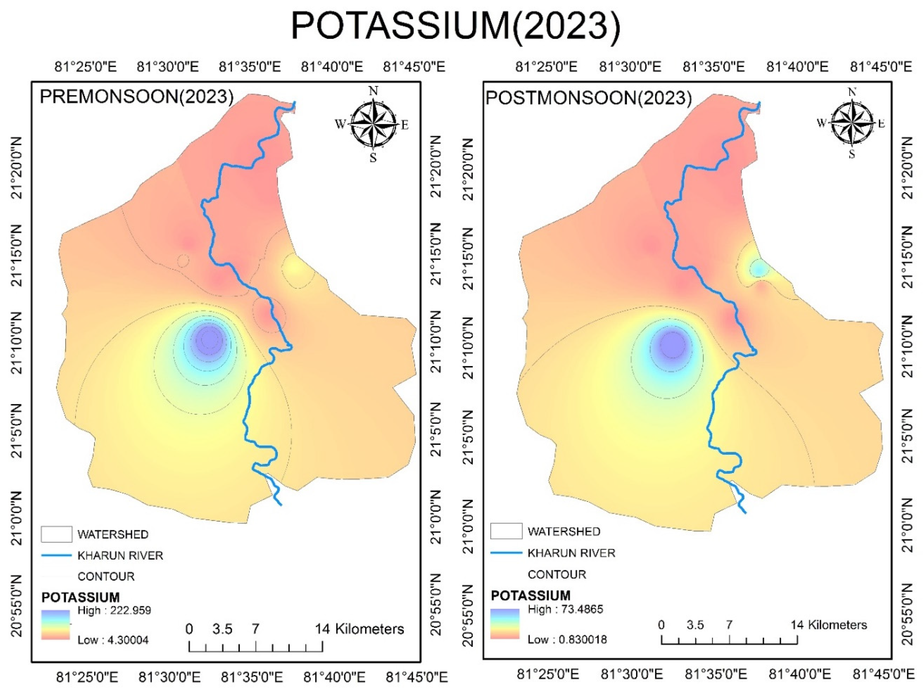
4.2.11. Potassium (K+)
4.3. Groundwater and Surface Water Interaction Study
4.3.1. Rock–Water Interaction Study
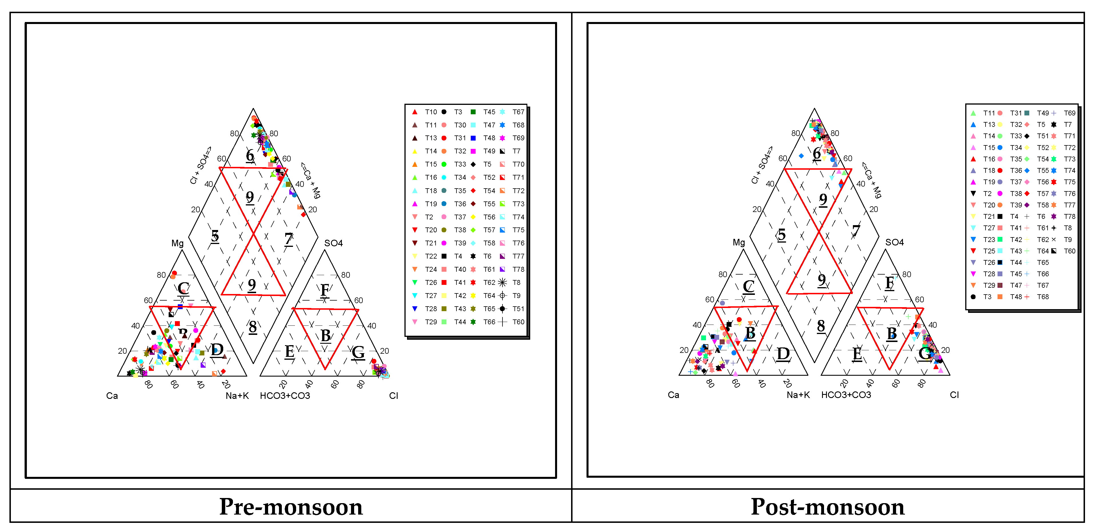
Piper Trilinear Diagram
Gibbs Diagram
4.3.2. Statistical Study
Pearson Correlation Analysis
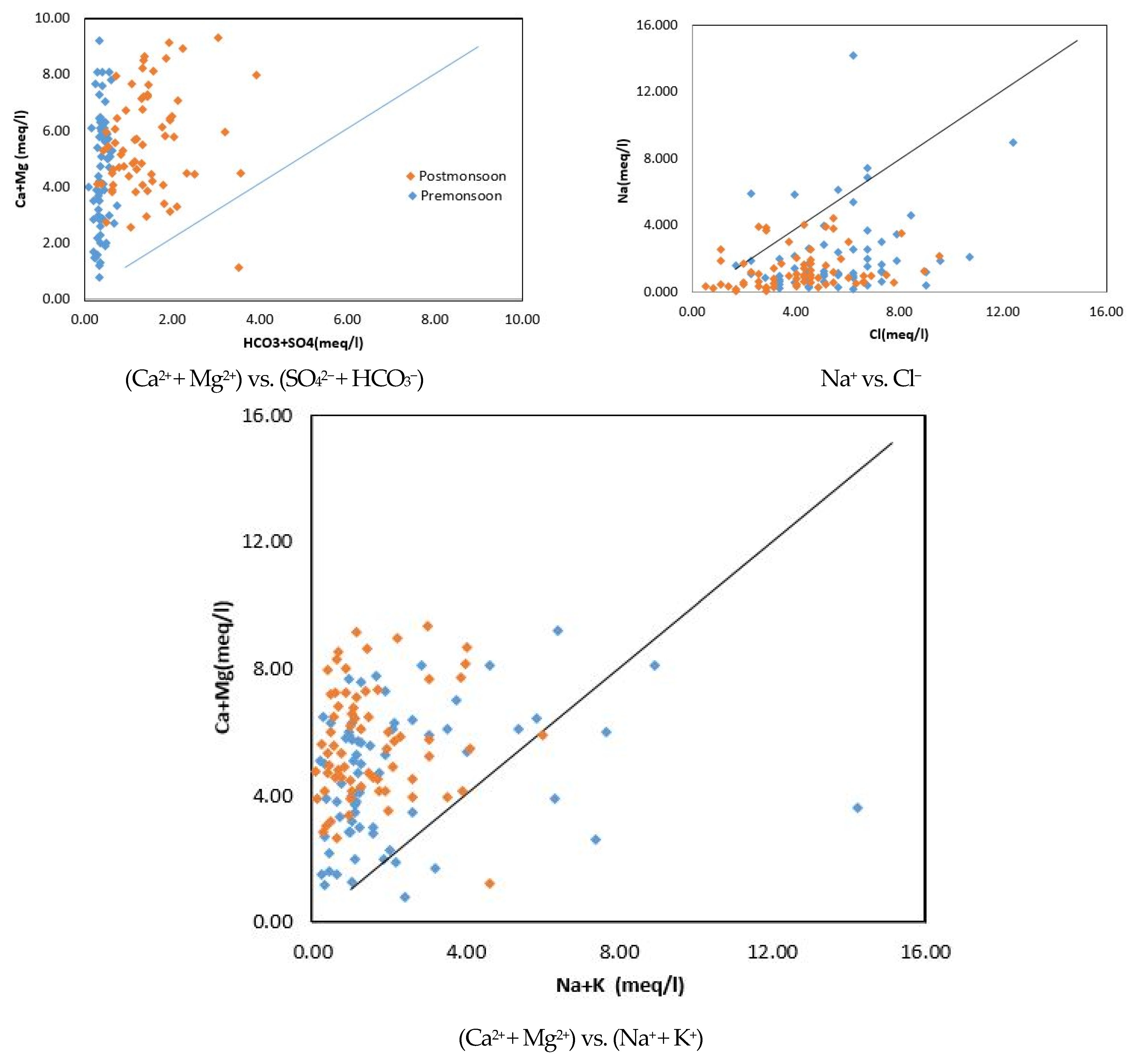
Scatter Plots
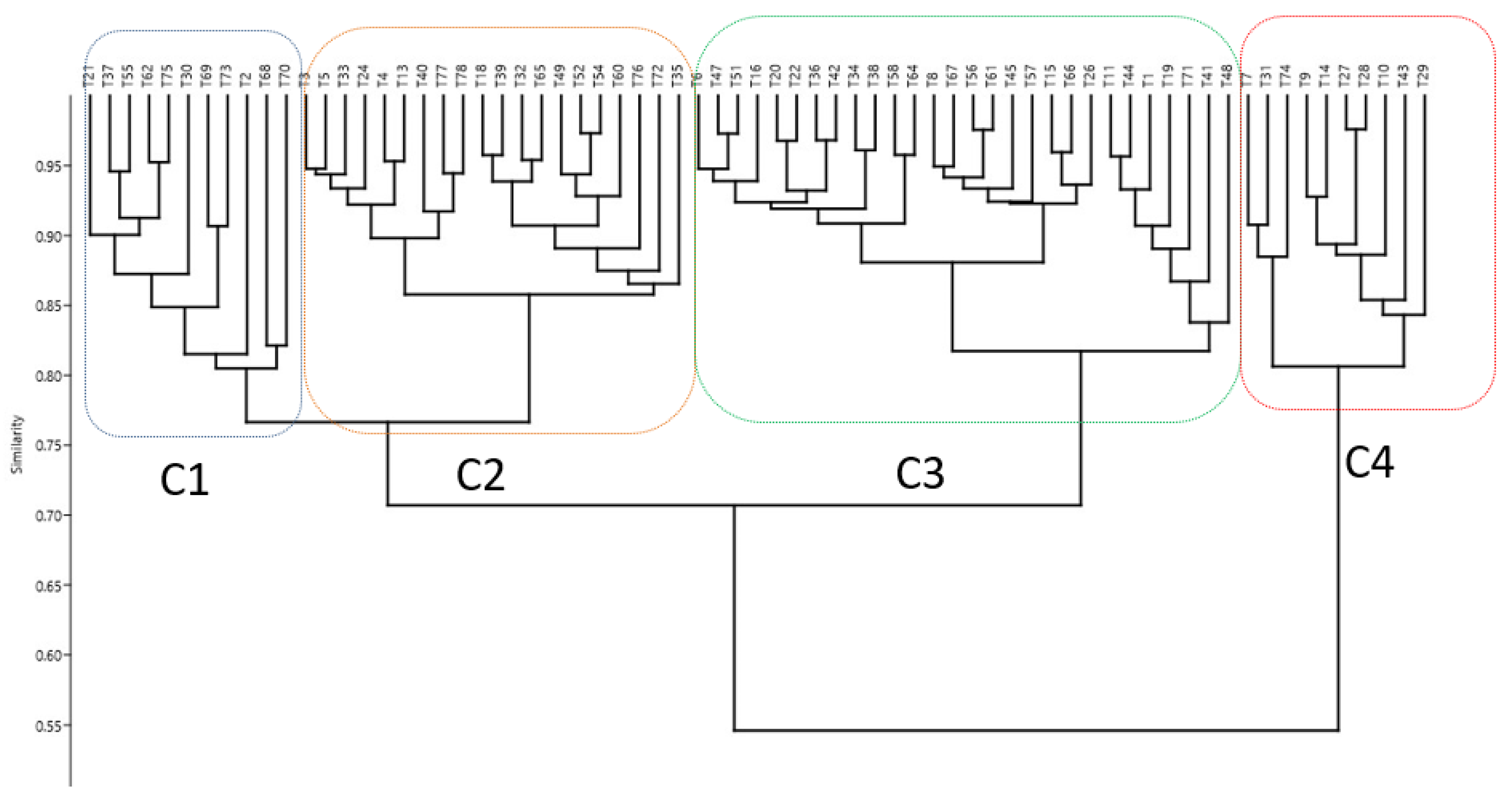
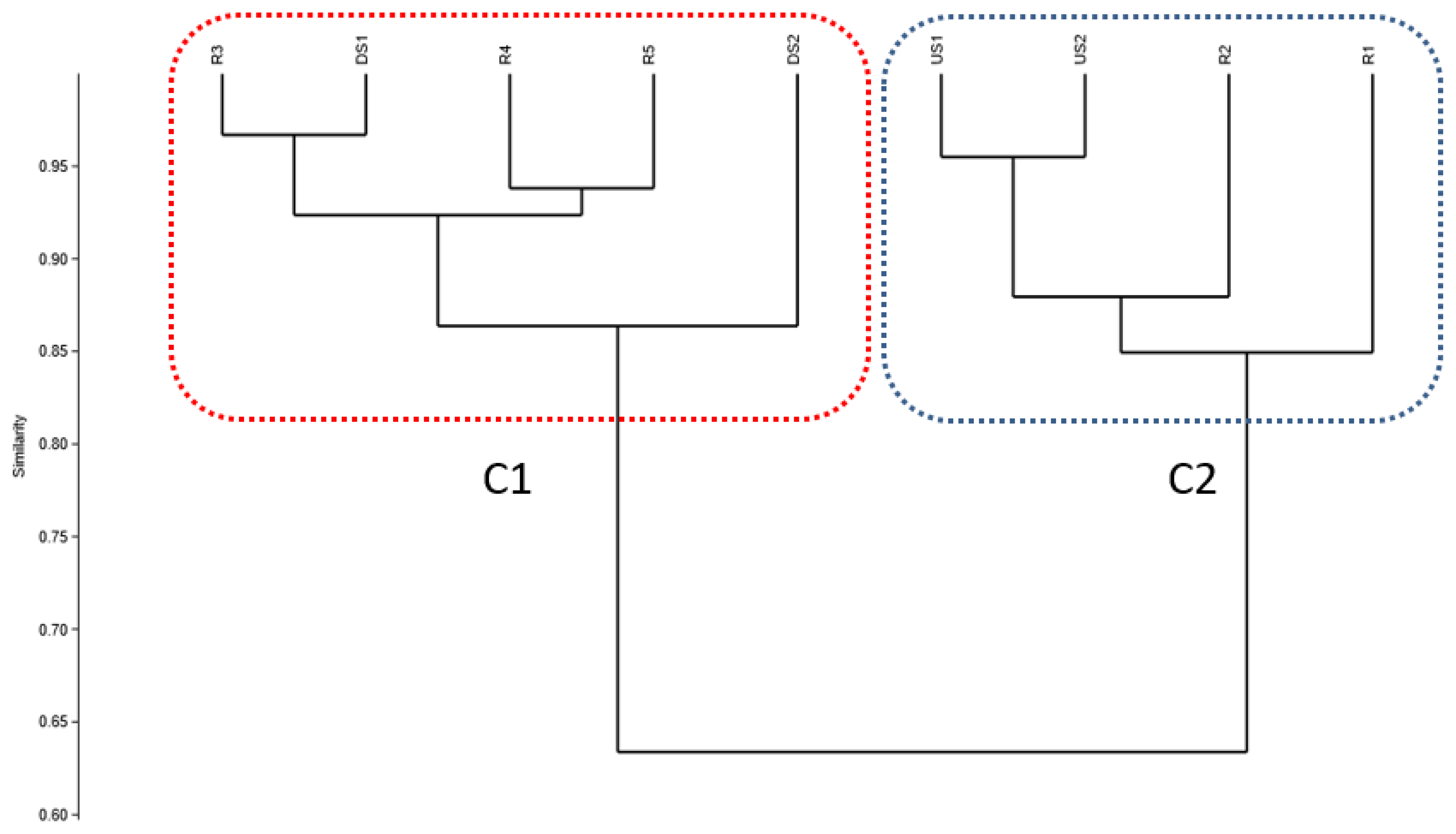
Hierarchical Cluster Analysis (HCA)
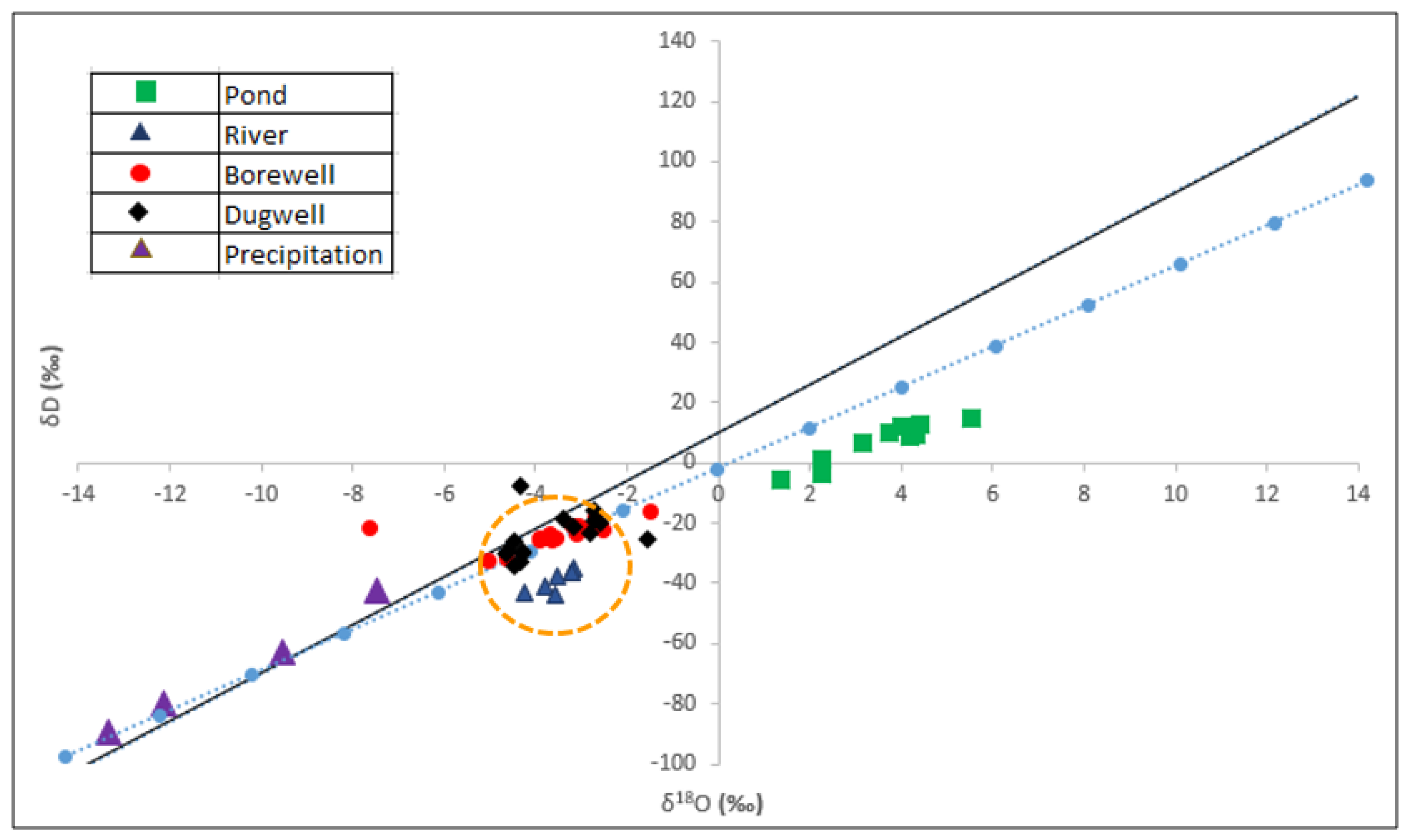
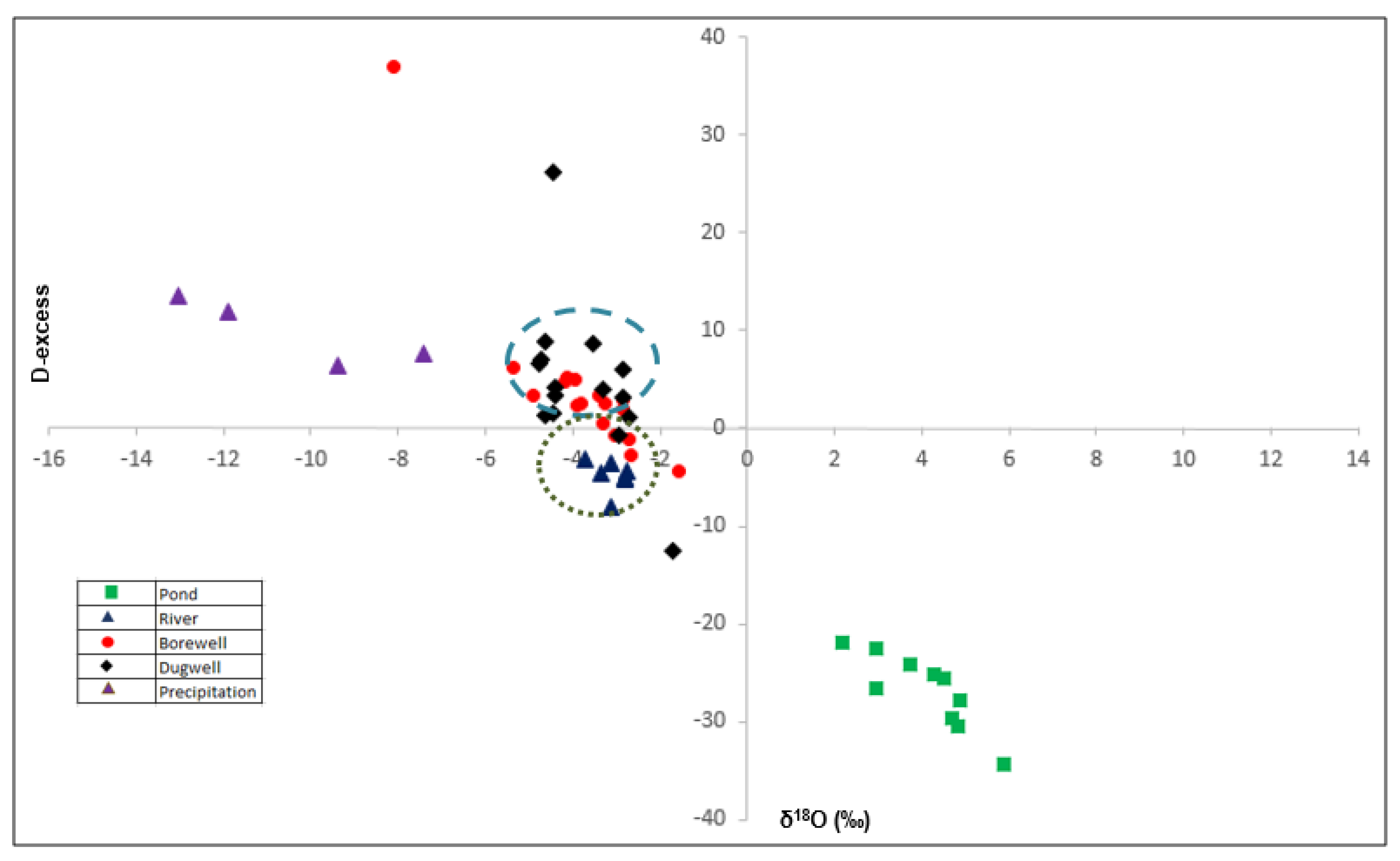
4.3.3. Stable Isotope Study
- a)
- Local Meteoric Water Line (LMWL) Development
- b)
- δ18O and δ2H Isotopic Composition of Precipitation
- c)
- δ18O and δ2H Isotopic Composition of Surface Water and Groundwater
- d)
- Deuterium Excess of the Samples
5. Conclusions
Author Contributions
Funding
Data Availability Statement
Acknowledgments
Conflicts of Interest
References
- Appleyard, S. The Impact of Urban Development on Recharge and Groundwater Quality in a Coastal Aquifer Near Perth, Western Australia. Hydrogeol. J. 1995, 3, 65–75. [Google Scholar] [CrossRef]
- Davila, P.R.A.; Leon, G.D.H.; Schuth, C. Urban impacts analysis on hydrochemical and hydrogeological evolution of groundwater in shallow aquifer Linares, Mexico. Environ. Earth Sci. 2012, 66, 1871–1880. [Google Scholar] [CrossRef]
- Dimitriou, E.; Moussoulis, E. Land use change scenarios and associated groundwater impacts in a protected peri-urban area. Environ. Earth Sci. 2011, 64, 471–482. [Google Scholar] [CrossRef]
- Krishan, G.; Singh, S.; Thayyen, R.J.; Ghosh, N.C.; Rai, S.P.; Arora, M. Understanding river–subsurface water interactions in upper Ganga basin, India. Int. J. River Basin Manag. 2020, 18, 243253. [Google Scholar] [CrossRef]
- Mohrlok, U.; Wolf, L.; Klinger, J. Quantification of infiltration processes in urban areas by accounting for spatial parameter variability. J. Soils Sediments 2008, 8, 34–42. [Google Scholar] [CrossRef]
- Mukherjee, A.; Babu, S.S.; Ghosh, S. Thinking about water and air to attain sustainable development goals during times of COVID-19 pandemic. J. Earth Syst. Sci. 2020, 129, 180. [Google Scholar] [CrossRef]
- Park, S.; Kim, S.; Yun, S.; Kim, S.; Chae, G.; Yu, S.; Kim, S.; Kim, Y. Effects of land use on the spatial distribution of trace metals and volatile organic compounds in urban groundwater, Seoul, Korea. Environ. Geol. 2005, 48, 1116–1131. [Google Scholar] [CrossRef]
- Scanlon, B.R.; Reedy, C.R.; Stonestrom, A.D.; Prudic, E.D.; Dennehy, F.K. Impact of land use and land cover change on groundwater recharge and quality in the southwestern US. Glob. Change Biol. 2005, 11, 1577–1593. [Google Scholar] [CrossRef]
- Shi, X.; Jiang, S.; Xu, H.; Jiang, F.; He, Z.; Wu, J. The effects of artificial recharge of groundwater on controlling land subsidence and its influence on groundwater quality and aquifer energy storage in Shanghai, China. Environ. Earth Sci. 2016, 75, 195. [Google Scholar] [CrossRef]
- Yan, B.; Xiao, C.; Liang, X.L.; Fang, Z. Arab J Impacts of urban land use on nitrate contamination in groundwater, Jilin City, Northeast China. Arab. J. Geosci. 2016, 9, 105. [Google Scholar] [CrossRef]
- Duttagupta, S.; Mukherjee, A.; Bhattacharya, A.; Bhattacharya, J. Wide exposure of persistent organic pollutants (PoPs) in natural waters and sediments of the densely populated Western Bengal basin, India. Sci. Total Environ. 2020, 717, 137187. [Google Scholar] [CrossRef]
- Duttagupta, S.; Mukherjee, A.; Das, K.; Dutta, A.; Bhattacharya, A.; Bhattacharya, J. Groundwater vulnerability to pesticide pollution assessment in the alluvial aquifer of Western Bengal basin, India using overlay and index method. Geochemistry 2020, 80, 125601. [Google Scholar] [CrossRef]
- Gourcy, L.L.; Groening, M.; Aggarwal, P.K. Stable oxygen and hydrogen isotopes in precipitation. In Isotopes in the Water Cycle; Springer: Dordrecht, The Netherlands, 2005; pp. 39–51. [Google Scholar]
- Shamsudduha, M. Groundwater resilience to human development and climate change in South Asia. In Global Water Forum (GWF) Discussion Paper; Global Water Forum: Canberra, Australia, 2013; Volume 1332. [Google Scholar]
- Yun, P.; Huili, G.; Demin, Z.; Xiaojuan, L.; Nobukazu, N. Impact of land use change on groundwater recharge in Guishui River Basin, China. Chin. Geogr. Sci. 2011, 21, 734–743. [Google Scholar]
- Cosgrove, D.M.; Johnson, G.S. Aquifer management zones based on simulated surface-water response functions. J. Water Resour. Plan. Manag. 2005, 131, 89–100. [Google Scholar] [CrossRef]
- Das, P.; Mukherjee, A.; Lapworth, D.J.; Das, K.; Bhaumik, S.; Layek, M.K.; Shaw, A.; Smith, M.; Sengupta, P.; MacDonald, A.M.; et al. Quantifying the dynamics of sub-daily to seasonal hydrological interactions of Ganges river with groundwater in a densely populated city: Implications to vulnerability of drinking water sources. J. Environ. Manag. 2021, 288, 11238. [Google Scholar] [CrossRef]
- Lewandowski, J.; Lischeid, G.; Nützmann, G. Drivers of water level fluctuations and hydrological exchange between groundwater and surface water at the lowland River Spree (Germany): Field study and statistical analyses. Hydrol. Process. 2009, 23, 2117–2128. [Google Scholar] [CrossRef]
- MacDonald, A.M.; Bonsor, H.C.; Ahmed, K.M.; Burgess, W.G.; Basharat, M.; Calow, R.C.; Dixit, A.; Foster, S.S.D.; Gopal, K.; Lapworth, D.J.; et al. Groundwater quality and depletion in the Indo-Gangetic Basin mapped from in situ observations. Nat. Geosci. 2016, 9, 762–766. [Google Scholar] [CrossRef]
- Maurya, A.S.; Shah, M.; Deshpande, R.D.; Bhardwaj, R.M.; Prasad, A.; Gupta, S.K. Hydrograph separation and precipitation source identification using stable water isotopes and conductivity: River Ganga at Himalayan foothills. Hydrol. Process. 2011, 25, 1521–1530. [Google Scholar] [CrossRef]
- Mukherjee, A. (Ed.) Groundwater of South Asia; Springer: Berlin/Heidelberg, Germany, 2018. [Google Scholar]
- Mukherjee, A.; Fryar, A.E.; Rowe, H.D. Regional-scale stable isotopic signatures of recharge and deep groundwater in the arsenic affected areas of West Bengal, India. J. Hydrol. 2007, 334, 151–161. [Google Scholar] [CrossRef]
- Mukherjee, A.; Saha, D.; Harvey, C.F.; Taylor, R.G.; Ahmed, K.M.; Bhanja, S.N. Groundwater systems of the Indian sub-continent. J. Hydrol. Reg. Stud. 2015, 4, 1–14. [Google Scholar] [CrossRef]
- Rosenshein, J.S. Region 18, Alluvial Valleys. In Hydrogeology; The Geological Society of North America: Boulder, CO, USA, 1988; pp. 165–175. [Google Scholar]
- Blanco-Coronas, A.M.; López-Chicano, M.; Calvache, M.L.; Benavente, J.; Duque, C. Groundwater-Surface Water Interactions in “La Charca de Suárez” Wetlands, Spain. Water 2020, 12, 344. [Google Scholar] [CrossRef]
- Wehrhahn, R.; Bercht, A.L.; Krause, C.L.; Azzam, R.; Kluge, C.L.; Strohschön, R.; Wiethoff, K.; Baier, K. Urban restructuring and social and water-related vulnerability in mega-cities—The example of the urban village of Xincún, Guangzhou (China). In Die Erde. Zeitschrift der Gesellschaft für Erdkunde zu Berlin; Geographical Society of Berlin: Berlin, Germany, 2008; Volume 139, pp. 227–249. [Google Scholar]
- Wiethoff, K.; Baier, K. Megacities Areas in Transition. Abandoned Sites as an Expression of a Continuously Changing mega-urban landscape. In Proceedings of the Megacities—Interactions Between Land Use and Water Management—Mitteilungen zur Ingenieurgeologie und Hydrogeologie, Guangzhou, China, 25–26 November 2009; Baier, K., Strohschön, R., Eds.; RWTH Publications: Aachen, Germany, 2009; Volume 99, pp. 83–92. [Google Scholar]
- Gangwar, S. Water Resource of India: From Distribution to Management. Int. J. Inf. Comput. Technol. 2013, 3, 845–850. [Google Scholar]
- Joshi, S.K.; Rai, S.P.; Sinha, R.; Gupta, S.; Densmore, A.L.; Rawat, Y.S.; Shekhar, S. Tracing groundwater recharge sources in the northwestern Indian alluvial aquifer using water isotopes (δ18O, δ2H and 3H). J. Hydrol. 2018, 559, 835–847. [Google Scholar]
- Bhat, N.A.; Jeelani, G. Quantification of groundwater–surface water interactions using environmental isotopes: A case study of Bringi Watershed, Kashmir Himalayas, India. J. Earth Syst. Sci. 2018, 127, 63. [Google Scholar] [CrossRef]
- Kumar, S.K.; Babu, S.H.; Rao, P.E.; Selvakumar, S.; Thivya, C.; Muralidharan, S.; Jeyabal, G. Evaluation of water quality and hydrogeochemistry of surface and groundwater, Tiruvallur District, Tamil Nadu, India. Appl. Water Sci. 2017, 7, 2533–2544. [Google Scholar] [CrossRef]
- Maharjan, M.; Donovan, J.J. Groundwater response to serial stream stage fluctuations in shallow unconfined alluvial aquifers along a regulated stream (West Virginia, USA). Hydrogeol. J. 2016, 24, 2003–2015. [Google Scholar] [CrossRef]
- Jat, M.K.; Khare, D.; Garg, P.K. Urbanization and its impact on groundwater: A remote sensing and GIS-based assessment approach. Environmentalist 2009, 29, 17–32. [Google Scholar] [CrossRef]
- Krishan, G.; Singh, S.; Sharma, A.; Sandhu, C.; Kumar, S.; Kumar, C.P.; Gurjar, S. Assessment of river Yamuna and groundwater interaction using isotopes in Agra and Mathura area of Uttar Pradesh, India. Int. J. Hydrol. 2017, 1, 86–89. [Google Scholar] [CrossRef]
- Madhuri, R.; Verma, M.K.; Tripathi, R.K. Impact of Urbanisation on water resources in Raipur city using GIS and Remote Sensing. Int. J. Earth Sci. Eng. 2012, 5, 1815–1819. [Google Scholar]
- Misra, A.K. Impact of Urbanization on the Hydrology of Ganga Basin (India). Water Resour. Manag. 2011, 25, 705–719. [Google Scholar] [CrossRef]
- Pandit, M.K.; Bhardwaj, V.; Pareek, N. Urbanization impact on hydrogeological regime in Jaipur Urban Block: A rapidly growing urban center in NW India. Environmentalist 2009, 29, 341–347. [Google Scholar] [CrossRef]
- Pradeep, K.N.; Jivesh, A.T.; Biranchi, N.D.; Arun, N.T. Impact of urbanization on the groundwater regime in a fast growing city in central India. Environ. Monit. Assess. 2008, 146, 339–373. [Google Scholar] [CrossRef]
- Rao, N.P.; Prasad, K.M.; Madhusudhan, B.J.; Krishna, V.S.R.; Anand, A.V.S.S.; Madhnure, P. Impact of Urbanization on Groundwater Quality in Vijayawada Urban Agglomeration, the New Capital Region of Andhra Pradesh, India—A Baseline Study. J. Geol. Soc. India 2016, 87, 539–552. [Google Scholar]
- Saumya, S.; Samaddar, A.B.; Srivastava, R.K.; Pandey, H.K. Ground Water Recharge in Urban Areas—Experience of Rain Water Harvesting. J. Geol. Soc. India 2014, 83, 295–302. [Google Scholar]
- Sharma, S.; Bharat, A.; Das, M.V. Study of Variations in Urban and Hydrological Components in Process of Urbanization. Int. J. Eng. Res. 2013, 2, 203–207. [Google Scholar]
- Singh, A.; Srivastav, K.S.; Kumar, S.; Chakrapani, J.G. A modified DRASTIC model (DRASTICA) for assessment of groundwater vulnerability to pollution in an urbanized environment in Lucknow, India. Environ. Earth Sci. 2015, 74, 5475–5490. [Google Scholar] [CrossRef]
- Wakode, H.B.; Baier, K.; Jha, R.; Ahmed, S.; Azzam, R. Assessment of Impact of Urbanization on Groundwater Resources using GIS Techniques—Case Study of Hyderabad, India. Int. J. Environ. Res. 2014, 8, 1145–1158. [Google Scholar]
- Das, S.; Nag, K.S. Application of multivariate statistical analysis concepts for assessment of hydrogeochemistry of groundwater—A study in Suri I and II blocks of Birbhum District, West Bengal, India. Appl. Water Sci. 2017, 7, 873–888. [Google Scholar] [CrossRef]
- Khan, N.M.M.S.; Kumar, R.A. Interpretation of groundwater quality using correlation and linear regression analysis from tiruchengode taluk, namakkal district, tamilnadu, India. J. Chem. Pharm. Res. 2012, 4, 4514–4521. [Google Scholar]
- Shroff, P.; Vashi, T.R.; Champaneri, A.V.; Patel, K.K. Correlation study among water quality parameters of groundwater of valsad district of south Gujarat (India). J. Fund. Appl. Sci. 2015, 7, 340–349. [Google Scholar]
- Kothari, V.; Vij, S.; Sharma, K.S.; Gupta, N. Correlation of various water quality parameters and water quality index of districts of Uttarakhand. Environ. Sustain. Indic. 2020, 9, 100093. [Google Scholar] [CrossRef]
- Bhat, S.A.; Meraj, G.; Yaseen, S.; Pandit, A.K. Statistical assessment of water quality parameters for pollution source identification in sukhnag stream: An inflow stream of lake wular (ramsar site), kashmir himalaya. J. Ecosyst. 2014, 2014, 898054. [Google Scholar] [CrossRef]
- Doza, B.; Islam, S.D.-U.; Rume, T.; Quraishi, S.B.; Rahman, M.S.; Bhuiyan, M.A.H. Groundwater quality and human health risk assessment for safe and sustainable water supply of Dhaka City dwellers in Bangladesh. Groundw. Sustain. Dev. 2020, 10, 100374. [Google Scholar] [CrossRef]
- Tokatli, C.; Kose, E.; Cicek, A.; Emiroglu, O.; Bastatli, Y. Use of cluster Analysis to evaluate surface water quality: An application from downstream of meric river basin (edirne, Turkey). Int. J. Adv. Sci. Eng. Technol. 2015, 3, 33–35. [Google Scholar]


| pH | Temp | Cond(EC) | TDS | Na | K | Mg | Ca | Fe | F | Cl | SO4 | HCO3 | NO3 | |
|---|---|---|---|---|---|---|---|---|---|---|---|---|---|---|
| pH | 1.00 | |||||||||||||
| Temp | 0.22 | 1.00 | ||||||||||||
| Cond | −0.41 | 0.08 | 1.00 | |||||||||||
| TDS | −0.41 | 0.08 | 1.00 | 1.00 | ||||||||||
| Na | −0.12 | −0.20 | 0.40 | 0.40 | 1.00 | |||||||||
| K | −0.23 | −0.14 | 0.17 | 0.17 | 0.20 | 1.00 | ||||||||
| Mg | −0.09 | 0.02 | 0.53 | 0.53 | 0.12 | 0.05 | 1.00 | |||||||
| Ca | −0.57 | −0.21 | 0.51 | 0.51 | 0.18 | 0.14 | −0.08 | 1.00 | ||||||
| Fe | −0.19 | −0.08 | 0.12 | 0.12 | 0.22 | 0.14 | −0.07 | 0.12 | 1.00 | |||||
| F | 0.26 | 0.13 | 0.17 | 0.17 | 0.22 | −0.03 | 0.14 | −0.21 | 0.25 | 1.00 | ||||
| Cl | −0.21 | 0.09 | 0.61 | 0.61 | 0.27 | −0.04 | 0.35 | 0.31 | 0.11 | 0.06 | 1.00 | |||
| SO4 | 0.04 | −0.14 | −0.09 | −0.09 | −0.17 | 0.04 | −0.04 | −0.14 | −0.12 | 0.07 | −0.10 | 1.00 | ||
| HCO3 | −0.38 | −0.17 | 0.25 | 0.25 | −0.01 | 0.05 | 0.08 | 0.36 | 0.13 | −0.06 | 0.21 | −0.04 | 1.00 | |
| NO3 | −0.39 | −0.39 | 0.29 | 0.29 | 0.22 | −0.04 | 0.14 | 0.43 | 0.05 | −0.17 | 0.25 | −0.08 | 0.29 | 1.00 |
| pH | Temp | Cond(EC) | TDS | Na | K | Mg | Ca | Fe | F | Cl | SO4 | HCO3 | NO3 | |
|---|---|---|---|---|---|---|---|---|---|---|---|---|---|---|
| pH | 1.00 | |||||||||||||
| Temp | 0.13 | 1.00 | ||||||||||||
| Cond | −0.04 | −0.26 | 1.00 | |||||||||||
| TDS | −0.04 | −0.26 | 1.00 | 1.00 | ||||||||||
| Na | 0.10 | −0.30 | 0.53 | 0.53 | 1.00 | |||||||||
| K | −0.18 | −0.34 | 0.36 | 0.36 | 0.12 | 1.00 | ||||||||
| Mg | −0.26 | 0.06 | 0.14 | 0.14 | 0.14 | 0.29 | 1.00 | |||||||
| Ca | −0.39 | −0.12 | 0.14 | 0.14 | −0.06 | −0.02 | −0.24 | 1.00 | ||||||
| Fe | 0.16 | 0.03 | −0.04 | −0.04 | −0.04 | 0.09 | −0.12 | 0.08 | 1.00 | |||||
| F | 0.13 | 0.02 | 0.20 | 0.20 | 0.27 | 0.23 | 0.10 | 0.01 | 0.07 | 1.00 | ||||
| Cl | −0.27 | −0.10 | 0.61 | 0.61 | 0.18 | 0.08 | 0.18 | 0.37 | −0.11 | 0.05 | 1.00 | |||
| SO4 | −0.20 | −0.11 | 0.43 | 0.43 | 0.11 | 0.24 | 0.16 | 0.07 | −0.07 | 0.22 | 0.44 | 1.00 | ||
| HCO3 | −0.01 | −0.41 | 0.47 | 0.47 | 0.32 | 0.32 | 0.07 | −0.16 | −0.16 | 0.13 | −0.01 | 0.06 | 1.00 | |
| NO3 | 0.00 | −0.02 | 0.07 | 0.07 | 0.05 | −0.08 | −0.25 | 0.17 | −0.10 | −0.30 | 0.09 | −0.12 | 0.03 | 1.00 |
| pH | Temp | Cond | TDS | Na | K | Mg | Ca | Cl | SO4 | HCO3 | NO3 | |
|---|---|---|---|---|---|---|---|---|---|---|---|---|
| pH | 1.00 | |||||||||||
| Temp | 0.45 | 1.00 | ||||||||||
| Cond | −0.87 | −0.42 | 1.00 | |||||||||
| TDS | −0.87 | −0.42 | 1.00 | 1.00 | ||||||||
| Na | −0.20 | 0.45 | 0.26 | 0.26 | 1.00 | |||||||
| K | −0.86 | −0.37 | 0.95 | 0.95 | 0.24 | 1.00 | ||||||
| Mg | −0.29 | −0.50 | 0.30 | 0.30 | −0.48 | 0.11 | 1.00 | |||||
| Ca | −0.52 | −0.08 | 0.66 | 0.66 | 0.59 | 0.77 | −0.47 | 1.00 | ||||
| Cl | −0.69 | −0.41 | 0.65 | 0.65 | 0.23 | 0.61 | −0.04 | 0.59 | 1.00 | |||
| SO4 | −0.75 | −0.77 | 0.53 | 0.53 | −0.40 | 0.53 | 0.54 | 0.04 | 0.46 | 1.00 | ||
| HCO3 | −0.19 | −0.20 | 0.17 | 0.17 | 0.35 | 0.08 | 0.08 | 0.18 | 0.16 | −0.11 | 1.00 | |
| NO3 | 0.27 | 0.04 | −0.68 | −0.68 | −0.26 | −0.63 | −0.01 | −0.63 | −0.45 | 0.09 | 0.02 | 1.00 |
| pH | Temp | Cond | TDS | Na | K | Mg | Ca | Cl | SO4 | HCO3 | NO3 | |
|---|---|---|---|---|---|---|---|---|---|---|---|---|
| pH | 1.00 | |||||||||||
| Temp | 0.46 | 1.00 | ||||||||||
| Cond | −0.88 | −0.45 | 1.00 | |||||||||
| TDS | −0.88 | −0.45 | 1.00 | 1.00 | ||||||||
| Na | −0.86 | −0.43 | 1.00 | 1.00 | 1.00 | |||||||
| K | −0.90 | −0.42 | 0.98 | 0.98 | 0.98 | 1.00 | ||||||
| Mg | −0.73 | −0.25 | 0.94 | 0.94 | 0.95 | 0.90 | 1.00 | |||||
| Ca | −0.89 | −0.53 | 0.98 | 0.98 | 0.98 | 0.96 | 0.91 | 1.00 | ||||
| Cl | −0.91 | −0.49 | 0.97 | 0.97 | 0.97 | 0.97 | 0.90 | 0.98 | 1.00 | |||
| SO4 | −0.67 | −0.25 | 0.54 | 0.54 | 0.53 | 0.69 | 0.39 | 0.51 | 0.63 | 1.00 | ||
| HCO3 | −0.64 | −0.13 | 0.54 | 0.54 | 0.51 | 0.50 | 0.42 | 0.51 | 0.53 | 0.42 | 1.00 | |
| NO3 | −0.79 | −0.51 | 0.81 | 0.81 | 0.79 | 0.83 | 0.72 | 0.83 | 0.88 | 0.62 | 0.30 | 1.00 |
| Type of Water | δ18O | δ2H | D-Excess | |||
|---|---|---|---|---|---|---|
| Min | Max | Min | Max | Min | Max | |
| Borewell | −7.35 | −1.52 | −32.884 | −16.42 | −4.26 | 36.54 |
| Dugwell | −4.6 | −1.66 | −34.47 | −8.244 | −12.75 | 25.99 |
| Pond | 2.19 | 5.85 | −4.266 | 12.712 | −34.087 | −21.786 |
| River | −3.53 | −2.66 | −32.21 | −25.83 | −8.21 | −3.459 |
| Precipitation | −13.055 | −7.40 | −90.91 | −51.50 | 6.431 | 13.524 |
Disclaimer/Publisher’s Note: The statements, opinions and data contained in all publications are solely those of the individual author(s) and contributor(s) and not of MDPI and/or the editor(s). MDPI and/or the editor(s) disclaim responsibility for any injury to people or property resulting from any ideas, methods, instructions or products referred to in the content. |
© 2025 by the authors. Licensee MDPI, Basel, Switzerland. This article is an open access article distributed under the terms and conditions of the Creative Commons Attribution (CC BY) license (https://creativecommons.org/licenses/by/4.0/).
Share and Cite
Jhariya, D.; Shrivastav, M.; Deshpande, R.D.; Padhya, V. Hydrological Dynamics of Raipur, Chhattisgarh in India: Surface–Groundwater Interaction Amidst Urbanization. Water 2025, 17, 930. https://doi.org/10.3390/w17070930
Jhariya D, Shrivastav M, Deshpande RD, Padhya V. Hydrological Dynamics of Raipur, Chhattisgarh in India: Surface–Groundwater Interaction Amidst Urbanization. Water. 2025; 17(7):930. https://doi.org/10.3390/w17070930
Chicago/Turabian StyleJhariya, Dalchand, Mayank Shrivastav, Rajendrakumar D. Deshpande, and Virendra Padhya. 2025. "Hydrological Dynamics of Raipur, Chhattisgarh in India: Surface–Groundwater Interaction Amidst Urbanization" Water 17, no. 7: 930. https://doi.org/10.3390/w17070930
APA StyleJhariya, D., Shrivastav, M., Deshpande, R. D., & Padhya, V. (2025). Hydrological Dynamics of Raipur, Chhattisgarh in India: Surface–Groundwater Interaction Amidst Urbanization. Water, 17(7), 930. https://doi.org/10.3390/w17070930