Sensitivity Analysis of Dissolved Oxygen in Cold Region Rivers Through Numerical Modelling

Abstract

Dissolved oxygen (DO) is one of the most critical water quality constituents in cold region rivers. Harsh winter conditions pose significant challenges for DO sampling, making numerical modeling a valuable tool for gaining insights into DO concentrations during winter. Sensitivity analysis is essential for understanding the relative importance of the model parameters to the DO concentrations; however, such studies are rare. This study conducted a DO sensitivity analysis in the Lower Athabasca River, Canada, using a water quality model with ice effects in the MIKE HYDRO River. The simulated flow, water level, water temperature and DO concentrations closely matched observed values along the study reach. A bidirectional perturbation analysis was conducted to assess the sensitivity of DO concentrations to 14 model parameters. The results indicate that photosynthesis and respiration are the two most influential processes affecting river DO under winter conditions despite lower biomass activity compared to open-water conditions. A distinct seasonal pattern was observed for most parameters, with DO sensitivity during winter ice-covered periods being significantly higher than in summer open-water conditions. The study provides valuable insights for the development of integrated water quality and ice models for cold region rivers.

1. Introduction

In cold regions, the annual cycle of various ice processes throughout winter in rivers and lakes, such as freeze-up, stable ice cover, and break-up, can significantly impact the hydrodynamics, sediment transport processes, and water quality constituents [1,2,3]. The impact is more pronounced in rivers due to higher flow rates and more complex geomorphology compared to lakes [4]. River ice processes can lead to increased water levels and reduced flow rates compared to open-water conditions [5,6]. The stable ice cover acts as a physical barrier on rivers, reducing incoming solar radiation and limiting light penetration to the water column. Simultaneously, it restricts heat exchange and reaeration between the water column and the atmosphere [5,7]. Consequently, water quality constituents, particularly dissolved oxygen (DO), are significantly affected during ice periods compared to ice-free conditions [8].

DO is one of the most critical indicators of the health of river aquatic ecosystems [9]. Given the inverse correlation of water temperature and DO, the annual minimum DO concentrations are typically observed during the open-water period, as documented in several case studies [10,11]. However, under winter conditions, DO concentrations tend to decrease from ice formation to the period of stable ice cover and then gradually increase, forming a sag trend throughout the winter season [9]. The decline in DO concentrations under ice is primarily caused by restricted reaeration, reduced biological activity from phytoplankton photosynthesis, and slower algae production [9,12]. The relatively low DO concentrations during this period can severely impact the habitat of aquatic organisms [9,12,13,14]. In addition to reduced photosynthesis and reaeration, which are major DO sources, slower decay rates of biochemical oxygen demand (BOD) and sediment oxygen demand (SOD) loads that are the primary DO sinks, further contribute to winter DO depletion [8,15]. Hence, continuous monitoring of DO concentrations under winter conditions is essential to gain insights into river ecosystems. Nevertheless, collecting DO data under harsh winter conditions is challenging due to the high safety risks and expenses involved [5]. In this context, numerical modeling can be highly valuable for hindcasting and predicting DO concentrations in cold regions.

While many studies have developed water quality models for DO, only a limited number address the impact of ice on DO through river ice processes. Recent water quality models, such as WASP [16,17,18] and CE-QUAL-W2 [18,19], have considered ice effects by restricting heat exchange and light penetration between the water column and the atmosphere. These models provide insights into how pollutants and climate change impact water quality, such as DO, dissolved organic carbon (DOC), total nitrogen (TN), total phosphorus (TP), and chlorophyll-a (CHLA) in ice-covered rivers. Efforts to simulate DO with ice cover at the current stage have been reported to rely on externally coupling one-dimensional (1D) ice process models with 1D and 2D water quality models [20,21]. Commonly applied river ice process models include MIKE-ICE [22], CRISSP1D [23], and River1D [5,24,25]. The external coupling method introduces errors when integrating the spatial and temporal distribution of ice coverage along the river and throughout the year from river ice models with water quality models. Therefore, a comprehensive model for simulating river ice processes and DO concentrations is essential. Ongoing research aims to integrate a water quality module into the University of Alberta’s public-domain river ice process model, River1D, to simulate DO under open-water and ice-affected conditions [26]. Developing such a model requires insights into the priority of processes involved in DO balance under winter conditions, which necessitates a sensitivity analysis of the simulated DO results with respect to changes in model parameters. Such analysis can help improve (i) monitoring efficiency, (ii) the selection of water quality modeling software, and (iii) estimations for modeling input parameters.

Parameter sensitivity analysis of a water quality model is generally performed using three methods: One-at-a-Time (OAT), the Morris Method, and Regional Sensitivity Analysis [27]. The OAT method is an example of local sensitivity analysis methodology, while the Morris Method and Regional Sensitivity Analysis are global sensitivity analysis methods. The key difference between local sensitivity analysis and global sensitivity analysis is that local sensitivity analysis typically evaluates the effect of small perturbations around a nominal point, making it suitable for linear systems or when focusing on key parameters with high sensitivity. In contrast, global sensitivity analysis considers the entire input space, accounting for interactions between parameters, and is more appropriate for complex, nonlinear systems [28,29]. Specifically, the OAT method is effective for understanding the impact of individual parameters on the output but ignores parameter interactions and is generally inappropriate for nonlinear models [27]. The Morris Method and Regional Sensitivity Analysis, while suitable for global and comprehensive exploration of nonlinear cases, require more complex datasets and greater computational costs [27].

Several studies have reported the sensitivity of DO results with respect to biological processes such as phytoplankton growth rate, nitrification, denitrification, BOD decay rate, and SOD using the OAT method under simulated ice cover [30,31,32]. These studies suggest that DO concentrations are sensitive to phytoplankton biomass parameters and SOD, and their sensitivity varies between ice-covered and open-water periods. Although SOD and phytoplankton generally decrease in winter due to low water temperatures, these processes can still influence winter DO concentrations. In some instances, phytoplankton biomass that is adequate to impact winter DO concentrations can increase under ice conditions, and SOD remains an important sink for DO [9,33,34]. The sensitivity of DO concentrations to biological processes such as photosynthesis, respiration, and reaeration requires further analysis to gain a broader understanding of the priority of parameters when constructing a comprehensive water quality and ice model, despite these processes being highly restricted by the presence of snow and ice cover [12,35].

This study presents a sensitivity analysis of river DO concentrations under both ice-covered and open-water conditions using a calibrated and validated one-dimensional (1D) water quality model with a simulated ice cover. The objectives are to (i) evaluate the sensitivity of DO to the input parameters in the numerical model for cold region rivers, (ii) gain insights into the dominant processes in DO balance under ice-covered and open-water conditions, and (iii) better understand the spatial and temporal effects of winter conditions on DO and compare DO under open-water and ice-covered conditions. This study provides insights to aid in the development of an integrated water quality and river ice processes model.

2. Materials and Methods

2.1. Study Reach and Data Availability

The Athabasca River originates in the Rocky Mountains and flows northeastward toward the Peace–Athabasca Delta and Lake Athabasca. This study focuses on the lower segment of the river, extending approximately 208 km from upstream of the Athabasca and Clearwater Rivers’ confluence near Fort McMurray to Old Fort, as illustrated in Figure 1. This section of the river exhibits complex morphology, characterized by both meandering and braided channel planforms with vegetated islands and bars. The study reach was chosen due to the availability of comprehensive datasets, including bathymetric, hydrometric, and water quality information, which are essential for model calibration and validation.

The model used in this study was built in the MIKE HYDRO River [20], which consists of 204 cross-sections, with each cross-section at approximately 1 km intervals. The model incorporates a total of 28 boundary conditions, including an inflow boundary located approximately 3 km upstream of the confluence of the Athabasca and Clearwater Rivers, 26 lateral inflow boundaries representing tributaries along the selected study reach, and an outflow boundary at the downstream end, as shown in Figure 1. All boundary conditions are input as a time series of discharge values except a constant value at the outflow boundary. The water quality data were obtained from the Canada–Alberta Joint Oil Sands Environmental Monitoring Information Portal (JOSMP) dataset [36]. Flow and water level data were obtained from Water Survey of Canada (WSC) station 07DA001 (Athabasca River below Fort McMurray), as well as Regional Aquatics Monitoring Program (RAMP) stations S24 (Athabasca River below Eymundson Creek) and S46 (Athabasca River near the Embarras Airport) [37]. Observed water temperature and dissolved oxygen (DO) concentrations were extracted from 7 stations within the JOSMP dataset and Alberta’s river water quality monitoring program (WQP) dataset [38]. These stations are designated as water temperature/DO sampling sites in Figure 1.

2.2. Model Description and Setup

MIKE, developed by the Danish Hydraulic Institute (DHI), has been widely applied in hydrodynamic and water resource studies. MIKE HYDRO, a sub-component in the system, provides a comprehensive framework for catchments, rivers, and floodplains, facilitating both hydrological and hydraulic assessments. The model applied in this study was constructed in MIKE HYDRO River, the 1D flow simulation module of MIKE HYDRO, which incorporates the hydrodynamic (HD) module for simulating flow dynamics and the advection–dispersion (AD) module for water quality analysis [39]. The MIKE ECO Lab module is employed alongside the AD module to simulate water quality, allowing for the use of either predefined DHI-supported templates or user-defined configurations [40]. The MIKE modeling system supports interconnectivity between modules, enabling users to address water modeling scenarios within a cohesive framework. However, the model lacks an ice simulation module, and therefore, modifications are necessary to simulate ice-cover effects for cold region rivers.

2.2.1. Hydrodynamic (HD)

The one-dimensional (1D) model in this study was configured in MIKE HYDRO River to simulate DO concentrations over a four-year period, from 1 January 2012 to 1 January 2016, with a 5-min computational timestep and a daily interval of outputs. The simulation period encompasses 5 winter seasons with ice cover effects and 4 summer seasons with open-water conditions. The initial portion of this period, from 1 January 2012 to 1 January 2014, was used for calibrating the simulated DO concentrations, while the latter segment, from 1 January 2014 to 1 January 2016, was used for validation. The hydrodynamic component of the model, which includes flow and water level, was calibrated and validated over the entire simulation period. The MIKE HYDRO River hydrodynamic (HD) module solves the 1D shallow water equations, also known as the Saint-Venant equations, using an implicit finite difference approach combined with the 6-point Abbott scheme [22]. The 1D conservation of mass and momentum equations are:

$$\left\{\begin{array}{c}{\displaystyle \frac{\partial A}{\partial t}}+{\displaystyle \frac{\partial Q}{\partial x}}=q\hfill \\ {\displaystyle \frac{\partial Q}{\partial t}}+{\displaystyle \frac{\partial }{\partial x}}\left({\displaystyle \frac{\alpha Q^2}{A}}\right)+gA{\displaystyle \frac{\partial h}{\partial x}}+{\displaystyle \frac{g{n}^{2}Q\left|Q\right|}{A{R}^{\frac{4}{3}}}}=0,\hfill \end{array}\right.$$

(1)

where Q is the discharge, A is the flow area, q is the lateral inflow, h is the water level above datum, R is the hydraulic radius, α is the momentum distribution coefficient, and n is Manning’s coefficient [21]; x is the space coordinate and t is the time coordinate. In this model, x = 0 is defined as the upstream boundary location.

2.2.2. Advection–Dispersion (AD) and Water Quality

The advection–dispersion (AD) component of the MIKE HYDRO River model represents the transport processes of individual water quality constituents. According to the user guide, the general form of the 1D advection–dispersion equation (which describes the conservation of mass for a dissolved substance) reads:

$${\displaystyle \frac{\partial AC}{\partial t}}+{\displaystyle \frac{\partial QC}{\partial x}}-{\displaystyle \frac{\partial }{\partial x}}\left(AD{\displaystyle \frac{\partial C}{\partial x}}\right)=-AKC+C_{2}q,$$

(2)

where C is the concentration, D is the dispersion coefficient, K is the linear decay coefficient, and C₂ is the source/sink concentration [22]. The −AKC term is the catchall term for the source/sink processes. The term C₂q accounts for the lateral inflow/outflow of the constituent being transported.

The water quality component of the model was developed and executed using the MIKE ECO Lab module. The DO balance is influenced by multiple processes, including ammonium processes, nitrate processes, BOD processes, and SOD. The governing equations for the source/sink terms of several water quality constituents consist of different ordinary differential equations. The governing equations are shown below [41].

DO Balance:

$${\displaystyle \frac{dDO}{dt}}=\stackrel{\mathrm{Photosynthesis} \& \mathrm{Respiration}}{\overbrace{P_{max}{S}_{input}{E}_f-R_{20}{{\Theta }_2}^{(T_w-20)}\Phi }}+\stackrel{\mathrm{Reaeration}}{\overbrace{K_a\left(C_s-DO\right){{\Theta }_{rear}}^{(T_w-20)}}}-\stackrel{\mathrm{BOD} \mathrm{decay}}{\overbrace{K_{d3}BOD{\Theta }_{d3}^{(T_w-20)}\Phi }}-\stackrel{\mathrm{Nitrification}}{\overbrace{Y_1{K}_4\left[N{H}_3\right]{\Theta }_4^{(T_w-20)}\Phi }},$$

(3)

Ammonium Processes:

$${\displaystyle \frac{d\left[N{H}_3\right]}{dt}}=\stackrel{\mathrm{Ammonia} \mathrm{Release} \mathrm{from} \mathrm{BOD} \mathrm{decay}}{\overbrace{Y_d{K}_{d3}BOD{{\Theta }_{d3}}^{(T_w-20)}\Phi }}-\stackrel{\mathrm{Nitrification}}{\overbrace{K_4\left[N{H}_3\right]{{\Theta }_4}^{(T_w-20)}\Phi }}-\stackrel{\mathrm{Uptake} \mathrm{by} \mathrm{plants}}{\overbrace{U_n\left(P_{max}{S}_{input}{E}_f-R_{resp}{{\Theta }_{resp}}^{(T_w-20)}\Phi \right){\Phi }_A}}-\stackrel{\mathrm{Uptake} \mathrm{by} \mathrm{bacteria}}{\overbrace{U_b{K}_{d3}BOD{{\Theta }_{d3}}^{(T_w-20)}\Phi }},$$

(4)

Nitrate Processes:

$${\displaystyle \frac{d\left[N{O}_3\right]}{dt}}=\stackrel{\mathrm{Nitrification}}{\overbrace{K_4\left[N{H}_3\right]{{\Theta }_4}^{(T_w-20)}\Phi }},$$

(5)

BOD Processes:

$${\displaystyle \frac{d\left[BOD\right]}{dt}}=-\stackrel{\mathrm{BOD} \mathrm{decay}}{\overbrace{K_{d3}BOD{{\Theta }_{d3}}^{(T_w-20)}\Phi }},$$

(6)

Temperature Processes:

$${\displaystyle \frac{d\left[T\right]}{dt}}=\stackrel{\mathrm{Net} \mathrm{solar} \mathrm{radiation}}{\overbrace{I_s-I_r}},$$

(7)

where P_max is the maximum oxygen production by photosynthesis; S_input is the fraction of maximum sunlight; E_f is the light extinction factor; R₂₀ is the respiration of animals and plants; Θ₂ is the Arrhenius temperature coefficient for respiration; Φ = DO²/(K_s + DO²); Φ_A = NH₃/(K_sn + NH₃); K_a = 5.233UD_w^1.67, is the reaeration coefficient; U is the flow velocity; D_w is the water depth; C_s is the oxygen saturation concentration; Θ_rear is the Arrhenius temperature coefficient for reaeration; K_d3 is the rate of BOD decay; Θ_d3 is the Arrhenius temperature coefficient for BOD decay; Y₁ is the oxygen demand by nitrification; K₄ is the rate of ammonia decay; Θ₄ is the Arrhenius temperature coefficient for nitrification; K_s is the half-saturation oxygen concentration; Y_d is the ratio of ammonia released at BOD decay; U_n represents uptake of ammonia by plants; K_sn is the half-saturation concentration for ammonia; U_b represents ammonia uptake by bacteria; I_s is the solar energy input; and I_r is the emitted heat loss.

Equations (3)–(7), along with their associated processes and parameters, were constructed in MIKE ECO Lab using the predefined template WQLevel3 with modifications [41]. These equations are the simplified version of the governing equations. The water quality component of the model omits SOD in the DO balance, denitrification in the nitrate processes, and sedimentation and resuspension in the BOD processes. Additionally, the ammonia uptake by plants term in the ammonium processes has been simplified. These simplifications were made because certain process parameters could not be adjusted within the MIKE ECO Lab template [20].

2.2.3. Ice-Cover Effects

The model used in this study does not incorporate or receive results from a river ice model. Instead, the MIKE HYDRO River model was modified to account for ice cover effects. Since the model does not simulate ice processes, the ice-covered period was specified as when the simulated water temperature T_w < 0.5 °C. This highlights the importance of accurate calibration and validation of water temperature in the water quality component of the model. For the ice cover period, the reaeration term K_a in Equation (3) was switched off to account for the gas exchange barrier effect of the ice cover.

The changes in flow resistance due to ice friction were accounted for by modifying the surface shear stress. This was achieved by applying wind friction to the water surface. A wind speed of up to 28.7 m/s was applied uniformly across all cross-sections of the study reach with a direction opposite to the flow direction. This wind friction was deactivated during open-water seasons. The wind friction repeats annually with the same starting and ending date, from 22 October to 27 April. The dates for modifying reaeration based on water temperature and wind friction are different in the model.

2.3. Sensitivity Analysis Methodology

Table 1. Model parameters, units, calibrated value, and testing range.

Parameter	Unit	Calibrated Value	Testing Range
Maximum oxygen production by photosynthesis, Pmax	gO2/m2/day	3.50	1.75–7.00
Respiration of animals and plants, R20	gO2/m2/day	3.0	1.0–5.0
Arrhenius temperature coefficient for respiration, Θ2	-	1.05	1.00–1.08
Arrhenius temperature coefficient for reaeration, Θrear	-	1.020	1.008–1.047
Rate of BOD decay, Kd3	1/day	0.25	0.10–1.50
Arrhenius temperature coefficient for BOD decay, Θd3	-	1.02	1.00–1.09
Oxygen demand by nitrification, Y1	gO2/gNH4	4.47	4.40–4.54
Rate of ammonia decay, K4	1/day	1.54	0–2.00
Arrhenius temperature coefficient for nitrification, Θ4	-	1.13	1.00–1.20
Half-saturation oxygen concentration, Ks	mg/L	2	0–20
Ratio of ammonia released at BOD decay, Yd	gNH4/gBOD	0.29	0.01–0.60
Uptake of ammonia by plants, Un	-	0.066	0–0.250
Uptake of ammonia by bacteria, Ub	-	0.109	0–0.250
Half-saturation coefficient for ammonia, Ksn	mg/L	0.05	0.01–1.00

summarizes all parameters assessed in this sensitivity analysis, along with their calibrated values and testing ranges determined based on previous research [20]. For parameters without a specified expected range, such as the half-saturation oxygen concentration, K_s, and the uptake of ammonia by plants and bacteria U_n and U_b, the suggested maximum and minimum values in MIKE ECO Lab were used as the upper and lower boundaries of the testing range. The reaeration rate was not included because the model calculates the reaeration coefficient K_a using an equation with constants that are not user-defined parameters.

The OAT method was used in this study. The calibrated values in Table 1 were used as the base case for the simulations. Bidirectional perturbation was applied, meaning that each parameter was adjusted to both a lower and a higher value in separate model simulations to assess the impact of decreasing and increasing the parameter on DO concentrations. During each perturbation, the values of other parameters were maintained at their base case (calibrated) values. Instead of applying a fixed ±10% change between the base case and perturbed values, which is a common threshold of the OAT method in previous studies [31], the minimum and maximum values for each parameter were selected to maximize the effect of the perturbation. A total of 14 parameters were analyzed in Table 1, leading to 28 sensitivity analysis cases. The sensitivity ε was proposed in this study to evaluate the impact of an individual parameter on the DO modeling results:

$$\epsilon (\mathrm{\%})={\displaystyle \frac{\mathsf{\Sigma }(D{O}_i-D{O}_{i\_B})}{\mathsf{\Sigma }D{O}_{i\_B}}}\times 100\%,$$

(8)

where DO_i is the DO concentration at time step i of the perturbed case, and DO_{i_B} is the DO concentration at time step i of the base case. The sensitivity analysis covered the entire simulation period, from 1 January 2012 to 1 January 2016. The classification of sensitivity followed the following criteria: (1) insensitive (I) if ε < 1%; (2) weakly sensitive (WS) if 1% < ε < 5%; (3) sensitive (S) if 5% < ε < 10%; and (4) highly sensitive (HS) if ε > 10% [42]. The simulation results were analyzed at four spatial locations along the study reach to have a comprehensive assessment at 50 km, 100 km, 150 km, and 200 km from the inflow boundary. At each location, the sensitivity values were calculated based on daily output DO concentrations. The sensitivities were assessed under both open-water and ice-covered conditions.

To better illustrate the seasonal variation in the DO sensitivity, seasonal sensitivity was calculated by separating the overall DO sensitivity analysis into five ice-covered and four open-water periods from 2012 to 2016, based on the calculated water temperature criterion (T_w < 0.5 °C as ice-covered periods). At each location, the sensitivity values were calculated for each corresponding period based on daily DO concentrations. The sum of all 5 winter period sensitivity values represents the ice-covered sensitivity at that specific location; a similar computation was carried out for open-water sensitivity. One single sensitivity value of the ice-covered periods and the open-water periods was calculated by averaging the results at all 4 locations for each case to focus on temporal effects. To show the contribution of winter ice-covered periods sensitivity to the overall sensitivity of DO concentrations, the contribution ratio was defined as:

$$Contribution Ratio={\displaystyle \frac{{\mathsf{\Sigma }(D{O}_i-D{O}_{i\_B})}_{ice}/\mathsf{\Sigma }D{O}_{i\_B}}{{\mathsf{\Sigma }\left(D{O}_i-D{O}_{i\_B}\right)}_{overall}/\mathsf{\Sigma }D{O}_{i\_B}}}={\displaystyle \frac{{\mathsf{\Sigma }(D{O}_i-D{O}_{i\_B})}_{ice}}{{\mathsf{\Sigma }\left(D{O}_i-D{O}_{i\_B}\right)}_{overall}}},$$

(9)

where ice represents the ice periods only and overall represents the overall time period. A value close to 1 indicates a more dominant ice-covered sensitivity compared to open-water sensitivity for the specific parameter. A higher contribution ratio indicates greater seasonal variation in DO sensitivity, reflecting a larger disparity in the contributions of ice-covered and open-water periods to overall sensitivity.

3. Results and Discussion

3.1. Calibration and Validation

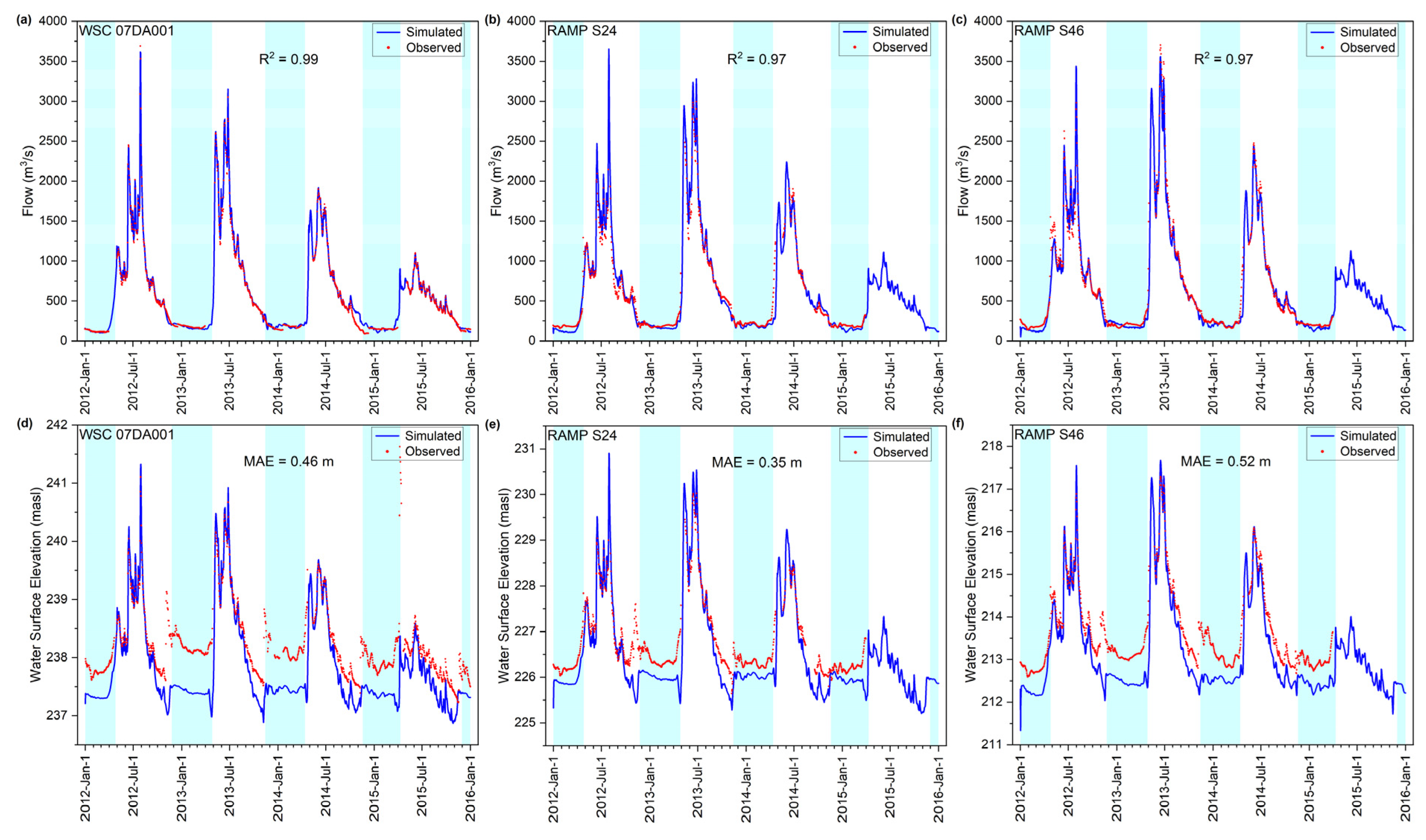
3.1.1. Flow and Water Level

Figure 2 presents the calibration and validation results for flow (m³/s) and water level (WSE, meters above sea level [masl]) at three stations with observed data, WSC 07DA001, RAMP S24, and S46, from 2012 to 2016. The blue shading represents ice-covered periods (the same for the following figures). The ice-covered period for each year was specified based on the dates when the gauge was affected by ice [43].

For the flow results, as Figure 2a–c shows, the coefficient of determination (R²) at all 3 stations is close to 1, indicating a strong correlation and a satisfactory fit between simulated and observed flow values. The simulated summer water levels closely matched the observed summer water levels, whereas the model underestimated water levels during winter ice-covered periods (Figure 2d–f).

This deviation was primarily caused by the displacement effect of the ice cover on water not being accounted for. The mean absolute error (MAE) at WSC 07DA001, RAMP S24, and S46 were 0.46 m, 0.35 m, and 0.52 m, respectively. The calibration and validation were deemed acceptable given the model’s limitation in representing ice effects and the similar error levels reported in the literature [5].

3.1.2. Water Temperature

Figure 3 shows that the modeled water temperatures agree very well with the observed ones under both open-water and ice-covered conditions, with R² values close to 1. This good fit of water temperature suggests that the ice-cover modification of switching on and off reaeration process indicated by the water temperature of the model (T_w < 0.5 °C) is appropriate, despite the fact that ice does not form until the water temperature drops below 0 °C in reality. However, the model predicts the start of the ice-covered periods earlier and the end later, similar to the flow and water level calibration and validation. In reality, the formation of stable ice cover takes several weeks instead of an instantaneous process indicated by water temperature only.

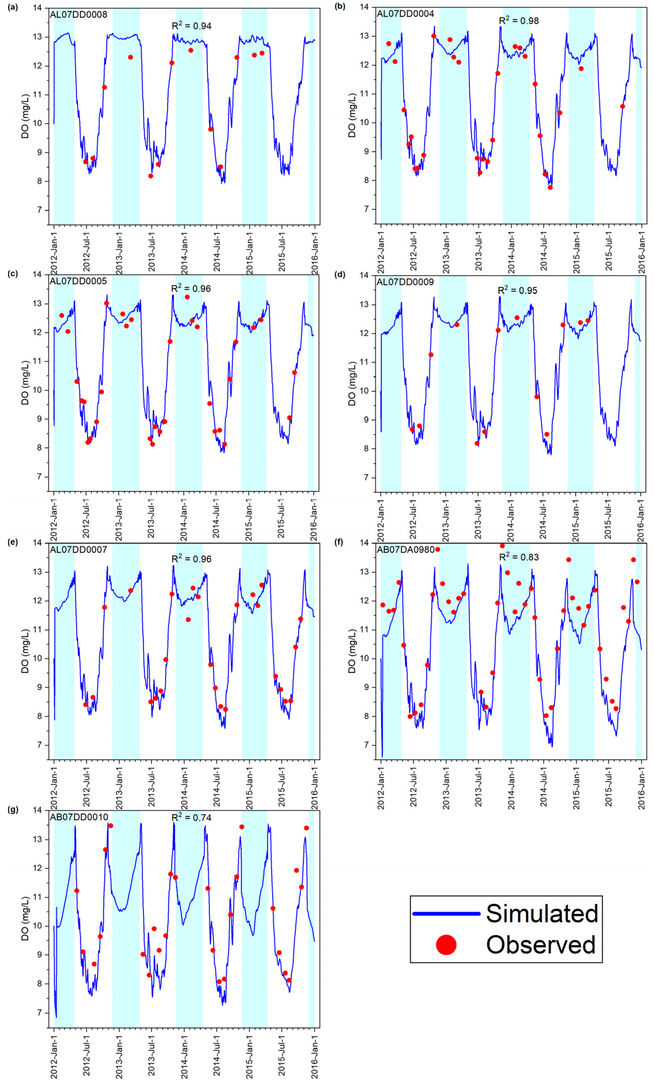
3.1.3. DO Concentration

Figure 4 presents the calibration and validation results of DO concentrations. The simulated values are closely aligned with the observed ones. The global minimum DO concentrations occurred in summer at all stations for both calibration (2012–2014) and validation (2014–2016). The reaeration process was active during open-water conditions, allowing light penetration and facilitating gas exchange between the water column and the atmosphere. Winter DO sags were more pronounced at downstream locations. It should be noted that the model switched off reaeration when T_w < 0.5 °C, which occurred earlier than the starting date of the actual ice period, as indicated by the blue shading in the figures. In reality, ice formation is a highly dynamic and spatially variable process, making the exact freeze-up date difficult to predict. Moreover, wind stress was applied on the water surface from 22 October to 27 April, the same dates annually, while the dates of water temperature below 0.5 °C vary each year, as discussed in Section 2.2.3, indicating that the two modifications for ice-cover effects in the model are inconsistent in terms of time.

The R² values are above 0.90 for the upstream 5 stations, while the last 2 stations fit less, with R² values of 0.83 and 0.74. At station AB07DA0980 (Figure 4f), the model consistently underestimated winter DO concentrations in the calibration period (2012–2014). This station, located 123 km downstream of the inflow boundary near the confluence of the Athabasca River and the Firebag River, exhibited slightly higher observed DO concentrations than other stations. The model also slightly underestimated DO at station AB07DD0010 (Figure 4g), which is close to the outflow boundary. Nevertheless, the model was deemed as satisfying, given the high R² values at all the stations.

3.2. Model Limitations

Several limitations exist in the model of this study. The primary limitation is that the ice cover is represented in a simplified manner, leading to inconsistencies in how ice processes influence the hydrodynamic and water quality results. The model applies a predefined wind time series to simulate ice friction but uses water temperature as a threshold for turning off reaeration. Because these two mechanisms operate independently, the timing of the ice effects in the hydrodynamics can be different from the time of the ice effects in the water quality calculations. This results in uncertainty in the simulated DO concentrations. Additionally, the wind time series is applied uniformly across the entire domain, and as a result, the spatial variability of ice cover that occurs in real rivers due to freeze-up and break-up processes is not captured.

Another limitation is that the model underpredicts the water levels. This causes uncertainty in the water velocities and, in turn, the water quality transport times. Additionally, the model does not account for the effects of the ice cover on light penetration, which can affect photosynthesis. It also does not account for the barrier effects of the ice cover on the heat exchange with the atmosphere, which can affect water temperature. These two omissions cause uncertainty in the simulated DO concentrations under ice conditions. The simplifications of the governing equations involving SOD processes is another limitation, given that the interaction between DO concentrations and SOD under winter conditions is complex, and previous studies have demonstrated that SOD may play a significant role [9,33,34].

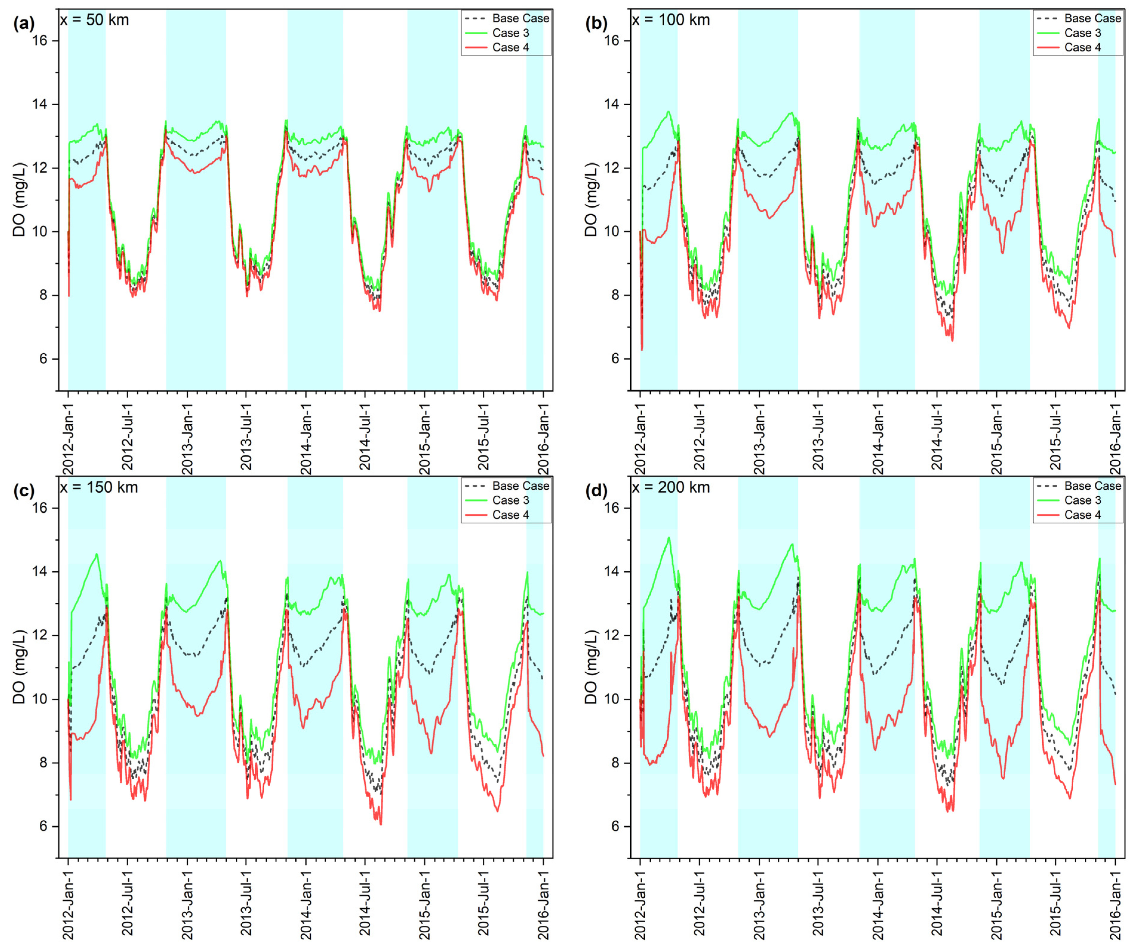
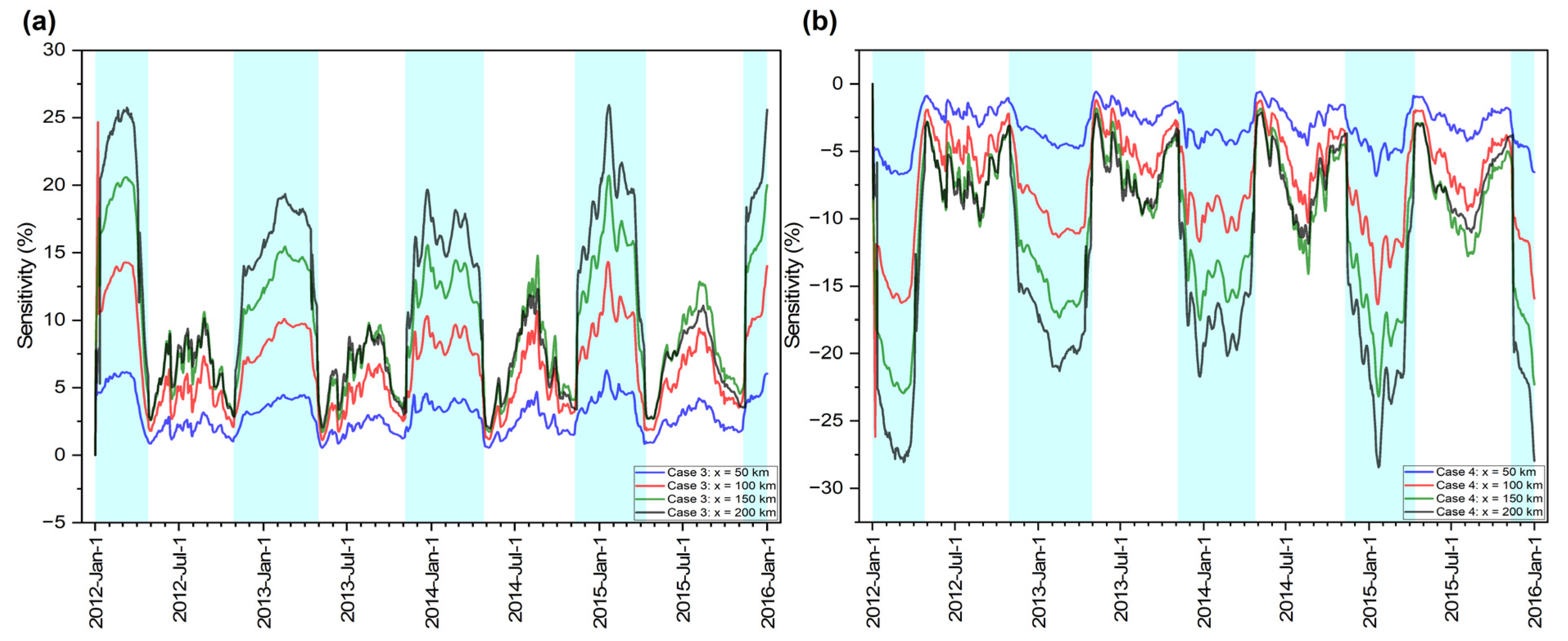
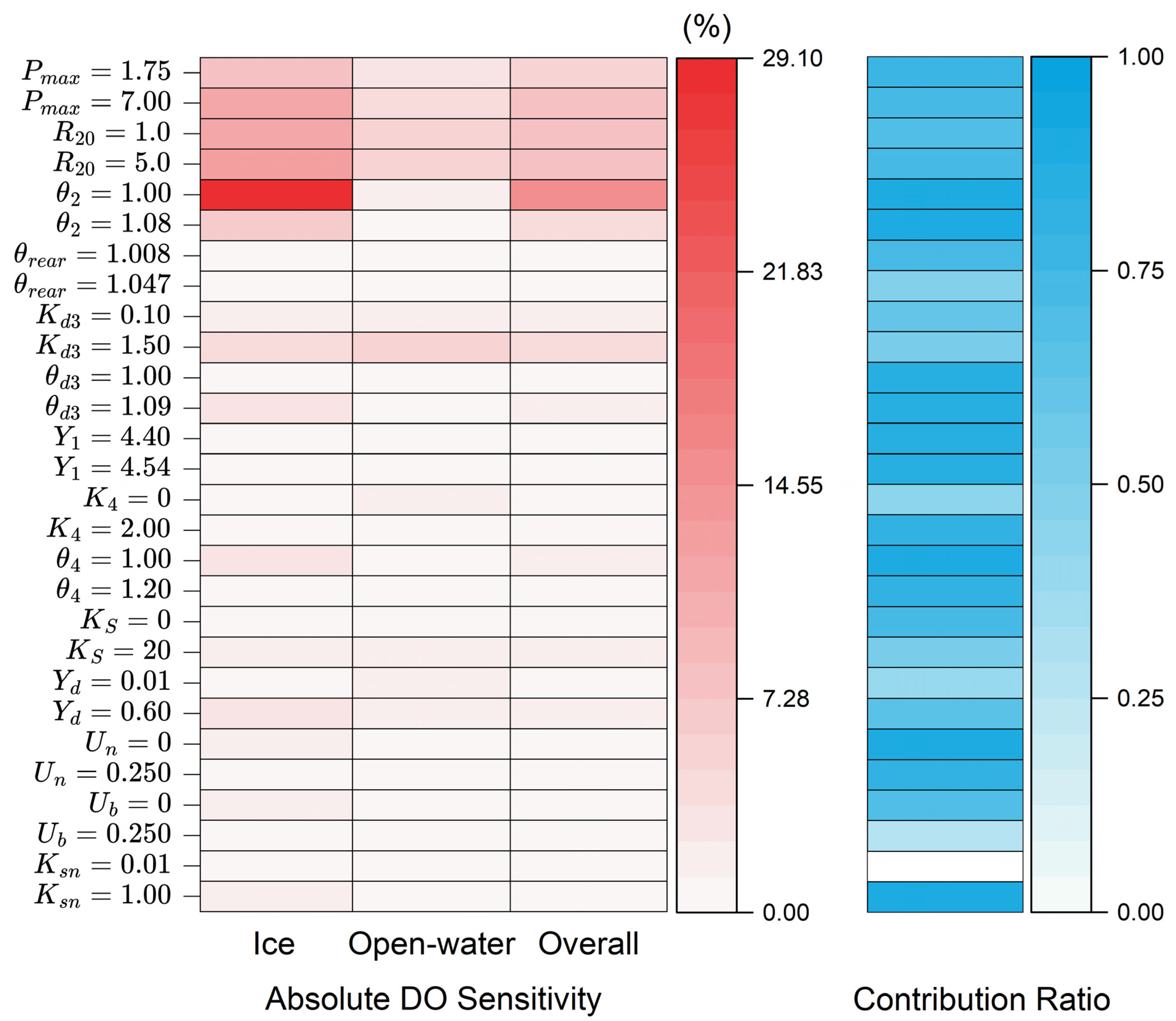
3.3. DO Sensitivity Analysis

Table 2. The average DO sensitivity results in 2012–2016 of all cases at x = 50 km, 100 km, 150 km, and 200 km.

	x = 50 km	x = 100 km	x = 150 km	x = 200 km
Case	Sensitivity (%)	Sensitivity (%)	Sensitivity (%)	Sensitivity (%)
Case 1: Pmax = 1.75	−1.83 (WS) *	−4.32 (WS)	−6.34 (S)	−7.54 (S)
Case 2: Pmax = 7.00	3.39 (WS)	7.24 (S)	10.48 (HS)	12.62 (HS)
Case 3: R20 = 1.0	3.01 (WS)	6.73 (S)	9.91 (S)	11.34 (HS)
Case 4: R20 = 5.0	−3.16 (WS)	−7.38 (S)	−10.85 (HS)	−12.33 (HS)
Case 5: Θ2 = 1.00	−5.70 (S)	−13.40 (HS)	−19.91 (HS)	−23.56 (HS)
Case 6: Θ2 = 1.08	1.45 (WS)	3.21 (WS)	4.80 (WS)	5.74 (S)
Case 7: Θrear = 1.008	−0.01 (I)	−0.19 (I)	−0.23 (I)	−0.22 (I)
Case 8: Θrear = 1.047	−0.19 (I)	−0.53 (I)	−0.84 (I)	−0.98 (I)
Case 9: Kd3 = 0.10	1.04 (WS)	2.04 (WS)	2.20 (WS)	2.01 (WS)
Case 10: Kd3 = 1.50	−4.71 (WS)	−5.77 (S)	−4.72 (WS)	−3.69 (WS)
Case 11: Θd3 = 1.00	−0.07 (I)	−0.31 (I)	−0.43 (I)	−0.46 (I)
Case 12: Θd3 = 1.09	1.04 (WS)	1.98 (WS)	2.10 (WS)	2.04 (WS)
Case 13: Y1 = 4.40	−0.07 (I)	−0.29 (I)	−0.41 (I)	−0.43 (I)
Case 14: Y1 = 4.54	−0.08 (I)	−0.33 (I)	−0.46 (I)	−0.48 (I)
Case 15: K4 = 0	0.45 (I)	1.06 (WS)	1.25 (WS)	1.13 (WS)
Case 16: K4 = 2.00	−0.19 (I)	−0.54 (I)	−0.67 (I)	−0.67 (I)
Case 17: Θ4 = 1.00	−1.22 (WS)	−2.07 (WS)	−2.28 (WS)	−2.26 (WS)
Case 18: Θ4 = 1.20	0.15 (I)	0.23 (I)	0.19 (I)	0.15 (I)
Case 19: Ks = 0	−0.18 (I)	−0.55 (I)	−0.77 (I)	−0.82 (I)
Case 20: Ks = 20	0.72 (I)	1.49 (WS)	2.06 (WS)	2.22 (WS)
Case 21: Yd = 0.01	0.26 (I)	1.02 (WS)	1.38 (WS)	1.29 (WS)
Case 22: Yd = 0.60	−0.47 (I)	−2.09 (WS)	−3.01 (WS)	−3.05 (WS)
Case 23: Un = 0	−0.19 (I)	−0.88 (I)	−1.33 (WS)	−1.49 (WS)
Case 24: Un = 0.250	0.12 (I)	0.27 (I)	0.30 (I)	0.30 (I)
Case 25: Ub = 0	−0.21 (I)	−0.91 (I)	−1.30 (WS)	−1.32 (WS)
Case 26: Ub = 0.250	0.10 (I)	0.41 (I)	0.56 (I)	0.52 (I)
Case 27: Ksn = 0	0.00 (I)	0.00 (I)	0.00 (I)	0.00 (I)
Case 28: Ksn = 1.00	−0.18 (I)	−0.80 (I)	−1.20 (WS)	−1.33 (WS)

* Notes: Abbreviations in the brackets stand for the classification standard of the sensitivity values: I = Insensitive, WS = Weakly Sensitive, S = Sensitive, and HS = Highly Sensitive.

presents the overall sensitivity analysis results of model parameter perturbations on DO concentrations for all 28 cases at the selected locations. Photosynthesis and respiration from biomass are the two most critical processes affecting the DO balance, as indicated by cases 1–6. The 3 related parameters, maximum oxygen production by photosynthesis (P_max), respiration of animals and plants (R₂₀), and the Arrhenius temperature coefficient for respiration (Θ₂), exhibited the highest sensitivity in both perturbation directions. The highest sensitivity was observed in case 5 at x = 200 km when Θ₂ = 1.00, decreased from the base case calibrated value of Θ₂ = 1.05, with a sensitivity value of −23.56%. The negative value indicates that the DO concentration was lower than the base case.

The general spatial trend observed across all parameters shows an increase in sensitivity from upstream to downstream. This is expected due to model initialization, spin-up process [44], and the fact that perturbations upstream influence conditions downstream. The increasing sensitivity trend from upstream to downstream is particularly pronounced for the sensitive parameters (P_max, R_20, and Θ₂) compared to other relatively insensitive parameters, such as those related to BOD and nitrification. For instance, the rate of BOD decay (K_d3) and the Arrhenius temperature coefficient for BOD decay (Θ_d3) were classified as weakly sensitive or insensitive at all four locations. Similarly, parameters associated with ammonium and nitrification processes, such as the oxygen demand by nitrification (Y₁), the rate of ammonia decay (K₄), and the Arrhenius temperature coefficient for nitrification (Θ₄), were generally either insensitive or weakly sensitive across all locations.

For each parameter, perturbations were examined in both directions—one decreasing and the other increasing from the base case value—resulting in 14 pairs of cases. As shown in Table 2, sensitivity values for each pair generally have opposite signs, indicating an inverse relationship with the base case results. For example, photosynthesis is expected to be positively correlated with DO concentrations because increasing the photosynthesis rate produces more oxygen, leading to higher DO concentrations, and vice versa. This relationship is evident in cases 1 and 2, where decreasing P_max from 3.50 to 1.75 (case 1) resulted in negative sensitivity values while increasing P_max to 7.00 (case 2) yielded positive sensitivity values.

The Arrhenius temperature coefficient for reaeration (Θ_rear) and the oxygen demand by nitrification (Y₁) were exceptions from the opposite trend shown in the two perturbation directions. In both cases (case 7,8 and case 13,14), negative sensitivity values were recorded for both perturbation directions. This is attributed to the extremely low sensitivity in these cases, and thus, DO concentration results remained nearly unchanged compared to the base case. Additionally, case 27 was a unique scenario where the half-saturation coefficient for ammonia K_sn = 0. This was equivalent to the base case, as its sensitivity was 0 across all locations.

To further illustrate the findings presented in Table 2, the respiration of animals and plants (R₂₀) was selected as a representative parameter. Figure 5 shows the DO concentration results in case 3 (R₂₀ = 1.0) and case 4 (R₂₀ = 5.0), along with the result from the base case, and Figure 6 shows the sensitivity at different locations. All other DO concentrations and sensitivity plots are available in the Supplementary Materials.

The blue shading in Figure 5 represents the ice periods when reaeration was turned off in the model, i.e., when the simulated water temperature T_w < 0.5 °C, different from the blue shadings in Figure 2, Figure 3 and Figure 4. In case 3, a reduction in R₂₀ led to increased DO concentrations during winter periods compared to the base case, whereas in case 4, an increase in R₂₀ resulted in the opposite trend. This confirms that respiration by animals and plants is negatively correlated with DO concentrations. The winter DO sags are clearly visible in case 4 in all years. The winter DO concentrations decreased in the downstream direction. The minimum DO concentration in ice-covered periods at 200 km from the upstream boundary was approximately 7 mg/L across all years, compared to 12 mg/L at 50 km. Moreover, the global minimum DO concentrations in both case 3 and case 4 occurred during open-water periods across all years, dropping below 8 mg/L. The open-water DO concentration patterns for both cases were nearly identical to the base case.

The trends in Figure 6 are consistent with those in Figure 5. Sensitivity values during winter periods were significantly higher than those during open-water conditions. The highest sensitivity values reached approximately ± 25% in both perturbation directions for R₂₀ in winter, while open-water values were around ± 10%. A clear spatial trend was also observed, with DO concentrations exhibiting greater sensitivity at downstream locations (x = 150 km and x = 200 km) than at upstream locations (x = 50 km and x = 100 km) across all years.

Using Figure 5 and Figure 6 as examples, it can be concluded that for parameter R₂₀, winter ice-covered periods dominated the overall sensitivity results presented in Table 2. These findings confirm the presence of seasonal variations in DO sensitivity. A seasonal sensitivity analysis is thus necessary to fully understand and compare DO concentrations between ice-covered and open-water conditions. The fact that photosynthesis and respiration are more dominant in winter compared to summer also provides explanations for high simulated winter DO concentrations compared to low simulated summer DO concentrations in terms of the water quality equations used in the model. In Equation (3), if the combined photosynthesis and respiration term, an overall source term of DO, is the most dominant in winter compared to other processes (reaeration, BOD decay, and nitrification), a high calculated DO concentration in winter should be expected.

Figure 7 presents the seasonal absolute DO sensitivity results and the contribution ratio for all parameters.

Figure 7 shows that seasonal differences in DO sensitivity are apparent for the majority of the model parameters, not just the highly sensitive parameters such as P_max, R₂₀, and Θ₂. The highest absolute sensitivity value was 29.02% when the Arrhenius temperature coefficient of respiration, Θ₂ = 1.00 during winter ice-covered periods, while the overall absolute sensitivity for this parameter was 15.64%. In nearly all cases, ice-covered sensitivity exceeded open-water sensitivity, with only two exceptions: (1) when the rate of BOD decay, K_d3 = 1.50, was perturbed in the positive direction from the base case, and (2) when the rate of ammonia decay K₄ = 0. This deviation from the general trend may be attributed to the increased biological activity in rivers during open-water periods. As one of the primary sink terms for DO in summer, the BOD decay rate plays a critical role in DO fluctuations across both seasons, contributing to global DO minima in summer and DO sags in winter [9]. As can be seen from Equations (3)–(6), K_d3 is involved in multiple processes, including BOD decay in the DO balance, ammonia release from BOD decay, and bacterial uptake in ammonium processes. Additionally, the BOD decay process is related to water temperature T_w, as well; see Equation (3). For the base case, in winter, assume T_w = 0 °C, ${\Theta }_{d3}^{(T_w-20)}$ = 0.67. This number is 1.00 in summer, assuming T_w = 20 °C. This means that in winter, the BOD decay process is about 67% of that in summer. Since the process itself is weaker, the DO results will naturally be less sensitive to changes in K_d3 during winter compared to summer. Other parameters related to nitrification were found to be insensitive in both ice-covered and open-water conditions, aligning with the spatial sensitivity results presented in Table 2.

Interestingly, the contribution ratio results revealed that even for insensitive parameters, seasonal variations in sensitivity were not only present but also significant. Almost all parameters displayed a high contribution ratio of above 0.60, which means that for most cases, ice-covered sensitivity is more pronounced than open-water sensitivity regardless of their sensitivity classification displayed in Table 2. Some expectation cases include Arrhenius temperature coefficient of reaeration Θ_rear = 1.047; rate of BOD decay K_d3 = 1.50; rate of ammonia decay, K₄ = 0, ratio of ammonia released at BOD decay, Y_d = 0.01, and uptake of ammonia by bacteria, U_b = 0.250. The contribution ratio values of these cases are between 0.20 and 0.50, suggesting that open-water periods are more dominant for these individual cases.

4. Conclusions and Future Work

Dissolved oxygen (DO) is one of the most critical water quality constituents in cold region rivers. This study conducted a sensitivity analysis of DO concentrations under winter conditions using a calibrated and validated one-dimensional (1D) numerical water quality model with ice-cover effects. The analysis was performed using the MIKE HYDRO River model coupled with the MIKE ECO Lab template to simulate DO variations in response to different parameter perturbations under both open-water and ice-covered conditions. The sensitivity of DO concentrations was assessed across various locations along the Lower Athabasca River, providing insight into key factors influencing winter DO dynamics.

The results suggested that the parameters associated with biological processes, particularly photosynthesis and respiration, exerted the greatest influence on DO concentrations. The maximum oxygen production by photosynthesis (P_max), respiration of animals and plants (R₂₀), and the Arrhenius temperature coefficient for respiration (Θ₂) were identified as the most sensitive parameters, with a highest sensitivity value of −23.56% for Θ₂ = 1.00. This indicates that, despite the constraints on biological activity due to ice and snow cover [12,35], these processes remain fundamental in governing DO balance in winter conditions. In contrast, parameters related to nitrification were found to have relatively weak or negligible sensitivity, suggesting that these processes play a lesser role in DO dynamics under ice-covered conditions. Sensitivity increased in the downstream direction, indicating a cumulative influence of the model spin-up period and upstream variations. A distinct seasonal pattern was observed in the sensitivity results, with ice-covered periods showing significantly higher contribution compared to open-water conditions for almost all parameters.

Future studies can focus on the following: (i) expanding the sensitivity analysis to include additional water quality constituents beyond DO and in other cold-region rivers, (ii) assessing the sensitivity of DO to variations in flow boundary conditions within the study reach, and (iii) developing a comprehensive water quality and ice model based on the sensitivity analysis results, emphasizing the most influential parameters.

References

1. Oveisy, A.; Rao, Y.R.; Leon, L.F.; Bocaniov, S.A. Three-dimensional winter modeling and the effects of ice cover on hydrodynamics, thermal structure and water quality in Lake Erie. J. Gt. Lakes Res. 2014, 40, 19–28. [Google Scholar] [CrossRef]
2. Turcotte, B.; Morse, B.; Bergeron, N.E.; Roy, A.G. Sediment transport in ice-affected rivers. J. Hydrol. 2011, 409, 561–577. [Google Scholar] [CrossRef]
3. Prowse, T.D. River-Ice Ecology. I: Hydrologic, Geomorphic, and Water-Quality Aspects. J. Cold Reg. Eng. 2001, 15, 1–16. [Google Scholar] [CrossRef]
4. Prowse, T.; Alfredsen, K.; Beltaos, S.; Bonsal, B.R.; Bowden, W.B.; Duguay, C.R.; Korhola, A.; McNamara, J.; Vincent, W.F.; Vuglinsky, V.; et al. Effects of Changes in Arctic Lake and River Ice. AMBIO 2011, 40, 63–74. [Google Scholar] [CrossRef]
5. Blackburn, J.; She, Y. A comprehensive public-domain river ice process model and its application to a complex natural river. Cold Reg. Sci. Technol. 2019, 163, 44–58. [Google Scholar] [CrossRef]
6. Nafziger, J.; She, Y.; Hicks, F. Dynamic River ice processes in a river delta network. Cold Reg. Sci. Technol. 2019, 158, 275–287. [Google Scholar] [CrossRef]
7. Hicks, F.E.; Phd, F.H. An Introduction to River Ice Engineering: For Civil Engineers and Geoscientists; CreateSpace Independent Publishing Platform: Scotts Valley, CA, USA, 2016; ISBN 978-1-4927-8863-8. [Google Scholar]
8. Chambers, P.A.; Brown, S.; Culp, J.M.; Lowell, R.B.; Pietroniro, A. Dissolved oxygen decline in ice-covered rivers of northern Alberta and its effects on aquatic biota. J. Aquat. Ecosyst. Stress Recovery 2000, 8, 27–38. [Google Scholar] [CrossRef]
9. Martin, N.; McEachern, P.; Yu, T.; Zhu, D.Z. Model development for prediction and mitigation of dissolved oxygen sags in the Athabasca River, Canada. Sci. Total Environ. 2013, 443, 403–412. [Google Scholar] [CrossRef]
10. Rajwa-Kuligiewicz, A.; Bialik, R.J.; Rowiński, P.M. Dissolved oxygen and water temperature dynamics in lowland rivers over various timescales. J. Hydrol. Hydromech. 2015, 63, 353–363. [Google Scholar] [CrossRef]
11. Williams, R.J.; Boorman, D.B. Modelling in-stream temperature and dissolved oxygen at sub-daily time steps: An application to the River Kennet, UK. Sci. Total Environ. 2012, 423, 104–110. [Google Scholar] [CrossRef]
12. Zdorovennova, G.; Palshin, N.; Golosov, S.; Efremova, T.; Belashev, B.; Bogdanov, S.; Fedorova, I.; Zverev, I.; Zdorovennov, R.; Terzhevik, A. Dissolved Oxygen in a Shallow Ice-Covered Lake in Winter: Effect of Changes in Light, Thermal and Ice Regimes. Water 2021, 13, 2435. [Google Scholar] [CrossRef]
13. Zhi, W.; Ouyang, W.; Shen, C.; Li, L. Temperature outweighs light and flow as the predominant driver of dissolved oxygen in US rivers. Nat. Water 2023, 1, 249–260. [Google Scholar] [CrossRef]
14. Whitfield, P.H.; McNaughton, B. Dissolved-oxygen depressions under ice cover in two Yukon rivers. Water Resour. Res. 1986, 22, 1675–1679. [Google Scholar] [CrossRef]
15. Pietroniro, A.; Chambers, P.A.; Ferguson, M.E. Application of a Dissolved Oxygen Model to an Ice-Covered River. Can. Water Resour. J. Rev. Can. Ressour. Hydr. 1998, 23, 351–368. [Google Scholar] [CrossRef]
16. Wool, T.; Ambrose, R.B.; Martin, J.L.; Comer, A. WASP 8: The Next Generation in the 50-year Evolution of USEPA’s Water Quality Model. Water 2020, 12, 1398. [Google Scholar] [CrossRef] [PubMed]
17. Żelazny, M.; Bryła, M.; Ozga-Zielinski, B.; Walczykiewicz, T. Applicability of the WASP Model in an Assessment of the Impact of Anthropogenic Pollution on Water Quality—Dunajec River Case Study. Sustainability 2023, 15, 2444. [Google Scholar] [CrossRef]
18. Terry, J.; Lindenschmidt, K.-E. Modelling Climate Change and Water Quality in the Canadian Prairies Using Loosely Coupled WASP and CE-QUAL-W2. Water 2023, 15, 3192. [Google Scholar] [CrossRef]
19. Wells, S.A. CE-QUAL-W2: A Two-Dimensional, Laterally Averaged, Hydrodynamic and Water Quality Model, Version 4.5 User Manual: Part 1 Introduction; Portland State University: Portland, OR, USA, 2024. [Google Scholar]
20. Shakibaeinia, A.; Kashyap, S.; Dibike, Y.B.; Prowse, T.D. An integrated numerical framework for water quality modelling in cold-region rivers: A case of the lower Athabasca River. Sci. Total Environ. 2016, 569–570, 634–646. [Google Scholar] [CrossRef]
21. Shakibaeinia, A.; Dibike, Y.B.; Kashyap, S.; Prowse, T.D.; Droppo, I.G. A numerical framework for modelling sediment and chemical constituents transport in the Lower Athabasca River. J. Soils Sediments 2017, 17, 1140–1159. [Google Scholar] [CrossRef]
22. DHI. A Modelling System for Rivers and Channels User Guide; DHI: Copenhagen, Denmark, 2012. [Google Scholar]
23. Chen, F.; Shen, H.T.; Jayasundara, N.C. A One-Dimensional Comprehensive River Ice Model. In Proceedings of the 18th IAHR International Symposium on Ice, Clarkson University, Potsdam, NY, USA, 28 August–1 September 2006; pp. 61–68. [Google Scholar]
24. Blackburn, J.; She, Y. One-dimensional channel network modelling and simulation of flow conditions during the 2008 ice breakup in the Mackenzie Delta, Canada. Cold Reg. Sci. Technol. 2021, 189, 103339. [Google Scholar] [CrossRef]
25. Blackburn, J.; She, Y. The simulation of ice jam profiles in multi-channel systems using a one-dimensional network model. Cold Reg. Sci. Technol. 2023, 208, 103796. [Google Scholar] [CrossRef]
26. Blackburn, J.; She, Y.; Zhang, W. Enhancing River1D for simulating water quality in ice-affected rivers. In Proceedings of the 27th IAHR International Symposium on Ice, Gdańsk, Poland, 9–13 June 2024. [Google Scholar]
27. Sun, X.Y.; Newham, L.T.H.; Croke, B.F.W.; Norton, J.P. Three complementary methods for sensitivity analysis of a water quality model. Environ. Model. Softw. 2012, 37, 19–29. [Google Scholar] [CrossRef]
28. Li, D.; Jiang, P.; Hu, C.; Yan, T. Comparison of local and global sensitivity analysis methods and application to thermal hydraulic phenomena. Prog. Nucl. Energy 2023, 158, 104612. [Google Scholar] [CrossRef]
29. Qin, C.; Jin, Y.; Tian, M.; Ju, P.; Zhou, S. Comparative Study of Global Sensitivity Analysis and Local Sensitivity Analysis in Power System Parameter Identification. Energies 2023, 16, 5915. [Google Scholar] [CrossRef]
30. Akomeah, E.; Chun, K.P.; Lindenschmidt, K.-E. Dynamic water quality modelling and uncertainty analysis of phytoplankton and nutrient cycles for the upper South Saskatchewan River. Environ. Sci. Pollut. Res. 2015, 22, 18239–18251. [Google Scholar] [CrossRef]
31. Hosseini, N.; Chun, K.P.; Wheater, H.; Lindenschmidt, K.-E. Parameter Sensitivity of a Surface Water Quality Model of the Lower South Saskatchewan River—Comparison Between Ice-On and Ice-Off Periods. Environ. Model. Assess. 2017, 22, 291–307. [Google Scholar] [CrossRef]
32. Hosseini, N.; Johnston, J.; Lindenschmidt, K.-E. Impacts of Climate Change on the Water Quality of a Regulated Prairie River. Water 2017, 9, 199. [Google Scholar] [CrossRef]
33. Terry, J.A.; Sadeghian, A.; Lindenschmidt, K.-E. Modelling Dissolved Oxygen/Sediment Oxygen Demand under Ice in a Shallow Eutrophic Prairie Reservoir. Water 2017, 9, 131. [Google Scholar] [CrossRef]
34. Akomeah, E.; Lindenschmidt, K.-E. Seasonal Variation in Sediment Oxygen Demand in a Northern Chained River-Lake System. Water 2017, 9, 254. [Google Scholar] [CrossRef]
35. Palshin, N.I.; Zdorovennova, G.E.; Zdorovennov, R.E.; Efremova, T.V.; Gavrilenko, G.G.; Terzhevik, A.Y. Effect of Under-Ice Light Intensity and Convective Mixing on Chlorophyll a Distribution in a Small Mesotrophic Lake. Water Resour. 2019, 46, 384–394. [Google Scholar] [CrossRef]
36. Canada-Alberta JOINT Oil Sands Environmental Monitoring Information Portal (JOSMP). Available online: https://www.canada.ca/en/environment-climate-change/services/oil-sands-monitoring.html (accessed on 10 December 2024).
37. Regional Aquatics Monitoring Program (RAMP). Available online: http://www.ramp-alberta.org/data/ClimateHydrology/climate/dailyClimate.aspx (accessed on 10 December 2024).
38. Alberta’s River Water Quality Monitoring Program (WQP). Available online: https://environment.extranet.gov.ab.ca/apps/WaterQuality/dataportal/ (accessed on 10 December 2024).
39. DHI MIKE HYDRO River User Guide. Available online: https://manuals.mikepoweredbydhi.help/latest/Water_Resources/MIKEHydro_River_UserGuide.pdf (accessed on 3 February 2025).
40. DHI. MIKE ECO Lab, Numerical Lab for Ecological and Agent Based Modelling User Guide. Available online: https://manuals.mikepoweredbydhi.help/latest/General/MIKE_ECO_Lab_UserGuide.pdf (accessed on 4 February 2025).
41. DHI WQ Templates, Scientific Description. Available online: https://manuals.mikepoweredbydhi.help/latest/General/MIKE_ECO_Lab_ShortScientific.pdf (accessed on 6 February 2025).
42. Chen, Q.S.; Xie, X.H.; Du, Q.Y.; Liu, Y. Parameters sensitivity analysis of DO in water quality model of QUAL2K. IOP Conf. Ser. Earth Environ. Sci. 2018, 191, 012030. [Google Scholar] [CrossRef]
43. Beltaos, S. Resistance of river ice covers to mobilization and implications for breakup progression in Peace River, Canada. Hydrol. Process. 2023, 37, e14850. [Google Scholar] [CrossRef]
44. Thornton, P.E.; Rosenbloom, N.A. Ecosystem model spin-up: Estimating steady state conditions in a coupled terrestrial carbon and nitrogen cycle model. Ecol. Model. 2005, 189, 25–48. [Google Scholar] [CrossRef]
Figure 1. Study reach of the Lower Athabasca River.
Water 17 01135 g001
Figure 2. Calibration and validation results of flow at stations (a) WSC 07DA001, (b) RAMP S24, (c) RAMP S46, and water level at the three stations (df).
Water 17 01135 g002
Figure 3. Model calibration and validation results of water temperature at seven stations.
Water 17 01135 g003
Figure 4. Model calibration and validation results of DO at seven stations.
Water 17 01135 g004
Figure 5. DO concentration results of the base case, case 3: R20 = 1.0 and case 4: R20 = 5.0 at cross-sections (a) x = 50 km; (b) 100 km; (c) 150 km; and (d) 200 km from 2012 to 2016.
Water 17 01135 g005
Figure 6. Sensitivity results of (a) case 3: R20 = 1.0 and (b) case 4: R20 = 5.0, at x = 50 km, 100 km, 150 km, and 200 km from 2012 to 2016.
Water 17 01135 g006
Figure 7. Seasonal absolute DO sensitivity and contribution ratio of all model parameters.
Water 17 01135 g007