Abstract
While 1D, 2D, and coupled 1D/2D models are widely used in flood extent mapping, a significant research gap remains in comparative analyses of 2D and coupled 1D/2D approaches. Study of the Dinsiz Stream Basin is of critical importance due to its proximity to industrial zones and residential areas, as well as its susceptibility to flood risk. Due to the lack and insufficiency of flow data in the basin, only long-term rainfall data were used in the analysis. Rainfall return periods of 50, 100, 200, and 500 years were estimated using statistical methods, and these values were utilized to generate flood hydrographs for this study. These values were then transferred to HEC-HMS, and the resulting hydrographs were input into HEC-RAS to establish coupled 1D/2D and 2D models for comparison. Flood mapping was performed for different return periods to evaluate the flood impact. This study revealed that maximum water levels in the 1D/2D models were higher than in the 2D models. The results showed that Dinsiz Stream could cause major losses for the second organized industrial zone located nearby when it overflows. The accuracy of the model was ensured with photographs of the flood event that occurred in 2021, ensuring the reliability of the findings.
1. Introduction
In recent years, many studies have been carried out on river floods, and more are currently ongoing. These studies highlight the increasing importance of understanding flood dynamics and improving flood management strategies. Therefore, it becomes imperative to delve further into flood studies and adopt new and contemporary approaches to address the evolving challenges in flood risk management.
Floods are regarded as among the most devastating natural disasters globally, having caused significant loss of life and property in recent decades. Flooding has also indirectly affected the economies of countries by creating negative environmental and socio-economic consequences [1,2]. In this context, addressing the severity of flood hazards worldwide requires sustained efforts [3]. Internationally, over the past 20 years, about USD 2.9 trillion was lost due to various natural disasters, and 1.3 million people died (1997–2018) [4]. Factors such as excessive rainfall, siltation in riverbeds, dam breakage with high discharge, and changes in drainage patterns are the main reasons for the frequency of floods [5]. Moreover, changes in land use affect hydrology, posing a heightened risk of flood occurrences [6,7].
In recent decades, many flood models have emerged, employing various hydrological approaches. These approaches can be categorized into empirical (data-driven), hydrodynamic, and physical process-based hydrological model types. The hydrodynamic approach employs mathematical equations to simulate the behaviour of fluids, derived by applying physical laws to fluid motions. This methodology can be categorized into 1D, 2D, and 3D models [8]. These models are apt for simulating floods of varying return periods [9]. The selection between 1D, 2D, or 1D/2D modelling depends on the desired results and the adequacy of available data. Many researchers have conducted comparisons between 1D and 2D modelling [10,11,12,13].
A straightforward representation of floodplain flow involves depicting the flow as one-dimensional along the river channel. One-dimensional flood models simulate flows assumed to travel longitudinally, such as in rivers and confined channels. While these models are computationally efficient, they face limitations, including the incapacity to simulate lateral diffusion of flood waves, subjectivity in cross-section location and orientation, and the discretization of topography as cross-sections rather than a continuous surface [8]. In such instances, 2D models are employed to simulate floodplain flow, providing a visualization that extends beyond what 1D models can provide. Two-dimensional models assume that water depth in the vertical direction can be disregarded compared with the other two dimensions. Nevertheless, to account for vertical features, vertical turbulence, vortices, and spiral flows [8], 3D models come into play. Three-dimensional models can surpass the limitations of 1D and 2D models by incorporating hydrostatic assumptions, viscous shear stresses, bed friction of fluid components, and other factors [14].
One of the crucial steps in conceptual flood mitigation measures is to create flood inundation maps. Mapping floodplain areas is a prerequisite for proper flood risk management and flood damage recovery [15]. Many researchers in different parts of the world have performed flood mapping and flood hazard assessment using HEC-RAS 5.0.7, a widely applicable computer software program. To generate maps, essential data such as topographic data, discharge data (profiles), Manning’s roughness coefficient, and geometric river sections (including river centreline, streamlines, riverbank lines, XS cutline) are required [16].
It is preferable to use one-dimensional models to model flows that are presupposed to flow in the longitudinal direction, such as rivers and closed canals, as these models are useful for calculation [8]. However, they cannot model the lateral diffusion of the flood wave, they decompose the topography in cuts rather than continuous surfaces, and the section location and orientation are not subjective [8]. The working principle of 2D models is that the third dimension, vertical water depth, can be neglected compared with the other two dimensions [17,18]. In general, 2D models are more accurate and reliable for complex flow simulations. Real-time flood forecasting via 2D models can be difficult; computations are slow and data-intensive [19]. Some flood modellers have developed new methods to eliminate long simulation times in 2D modelling [19,20]. Among these, the coupled 1D/2D method developed by HEC-RAS is one of the most used and preferred. In coupled approaches, 1D and 2D models can be linked together and the river and floodplain relationship is powerfully demonstrated [21].
The use of coupled 1D and 2D models improves the quality of results [22,23] and saves computer memory and time, which limit 2D models [24]. The complexity and quality of topographic data and inputs influence the results of these models [25,26]. A number of recent studies involving the development of coupled 1D/2D flood modelling are reviewed in this paper. Sönmez and Doğan [27] determined the flood inundation area in Cedar River using calibrated and validated 1D and 1D/2D models. Betsholtz and Nordlöf [28] investigated the potential and limitations of 1D, 2D, and coupled 1D/2D flood modelling in HEC-RAS, using the Höje River as a case study. Hammami et al. [29] used a coupled 1D/2D HEC-RAS model to assess the impact of dredging works on the Medjerda River floods in Tunisia. Kalra et al. [30] carried out coupled 1D and 2D HEC-RAS floodplain modelling of the Pecos River in New Mexico. Dasallas et al. [31] modelled a coupled HEC-RAS 1D/2D simulation to investigate the 2002 Baeksan flood event in Korea.
A coupled 1D/2D model employs a 1D model to replicate the movement and water depth in the primary flow of the river, and a 2D model to emulate flooding on the floodplain. Despite the historical demonstration of effective performance by this hydrodynamic model type, contemporary hydrodynamic inundation models generally adopt a purely 2D approach. They utilise unorganized (i.e., irregular or flexible) grids to delineate intricate geometries [8,32].
The latest methodology is the coupled 1D/2D technique pioneered by the U.S. Army Corps of Engineers Hydrologic Engineering Center River Analysis System (HEC-RAS), a widely utilised 1D river simulation model. This integrated approach facilitates connection between the 1D and 2D models, enabling dynamic representation of river and floodplain interactions [21]. Utilisation of coupled 1D/2D models for hydraulic/hydrodynamic simulation is a relatively recent feature in the HEC-RAS 5.0.7 hydraulic software, and only a handful of researchers have explored this approach for flood simulation analysis [33,34,35].
Ucar et al. [36] conducted comprehensive flood risk assessment in the Susurluk Basin, Türkiye, using hydrological modeling (HEC-HMS), HEC-RAS 1D and 2D hydraulic models, and GIS-based flood mapping aligned with the EU Flood Directive. They developed 503 hydrodynamic models (226 1D and 277 2D), analyzing 2116 km of stream length, and found that only 33 streams had sufficient capacity, while 470 high-risk areas required urgent intervention. That study highlights the vulnerability of critical infrastructure in urban centers and provides a data-driven framework for flood risk mitigation, including both structural and non-structural measures.
Specifially, Vozinaki et al. [13] pointed out that by presenting comprehensive hydraulic results for each grid point in the computed mesh of a river’s floodplains, using coupled 1D/2D modelling (with high-resolution DEM), additional insights can be obtained regarding inundation areas and the accuracy of water depth values in flood-prone regions.
Recent research has compared the performance of 1D, 2D, and 1D/2D hydrodynamic models for flood modeling and risk assessment. Kulkarni and Kale [37] developed a combined 1D/2D model using HEC-RAS to address flooding in the Panchganga River basin, demonstrating that the 1D/2D combined HEC-RAS model accurately predicted flood depth and extent.
Siakara et al. [38] compared 1D/2D and fully 2D models in urban and rural areas of Cyprus, concluding that 2D models were more flexible and effective in mitigating flood impacts. Similarly, Lim et al. [39] analyzed the Way-Ela dam failure in Indonesia, finding that 2D models provided the most accurate results, while 1D/2D models produced comparable outcomes but required longer computational times.
Moghim et al. [40] investigated two basins with varying topography, using HEC-RAS and LISFLOOD-FP software, finding that 2D models offered higher accuracy. The study also emphasized the influence of input parameters such as digital elevation models (DEM)s and roughness coefficients on simulation performance.
This study addresses an important gap in the existing literature by investigating the use of coupled 1D/2D models in HEC-RAS, especially in areas where historical flood data are limited. While many studies have focused on 1D or 2D models independently, there is still a lack of research on combining both approaches, especially in complex floodplain areas. This study compares the results of the coupled 1D/2D model with a fully 2D model, in which context relatively little detailed research has been carried out, especially when it comes to flood hazard mapping and inundation areas. The innovative aspect of this study is its testing of the flood event of July 2021 using real rainfall data and models constructed for different flood return periods (50, 100, 200, and 500 years). Thus, it contributes to the ongoing debate on the accuracy and efficiency of coupled 1D/2D models and 2D flood models.
This study critically examines the disparities between flood inundation maps generated using 2D models and those derived from the coupled 1D/2D HEC-RAS models. By evaluating flood scenarios corresponding to different return periods, the study provides comprehensive flood maps for the area. These maps not only emphasize the significant impact of modeling approaches on flood predictions but also serve as a crucial tool for informed hydrological management, offering essential insights for effective flood risk assessment and planning in the study area.
2. Data Collection, Materials, and Methods
This study consisted of two steps: hydrological and hydraulic. The calculation of rainfall data, flow data, and soil data contributed to the hydrological step, the flood maps were generated during the hydraulic step. The flowchart of this study is presented in Figure 1.
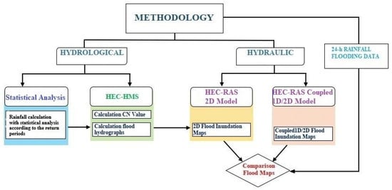
Figure 1.
The flowchart of study.
2.1. Study Area
The Sakarya Basin is one of the 25 hydrological basins in Türkiye. It is located between latitude 37°96′–41°20′ north and longitude 29°26′–33°24′ east. The drainage basin area covers 58,160 km2, accounting for about 7% of the land area of Türkiye. The distance between the ends of the basin boundary is approximately 378 km in the north–southeast direction and 340 km in the east–west direction. The Sakarya Basin has a mean slope of approximately 0.78. The basin is completely filled with river sediments and today a large part of it is agricultural land [41]. Figure 2 shows the Dinsiz Stream basin and the location of this study.
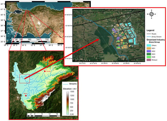
Figure 2.
The location of Dinsiz Stream, Sakarya.
2.2. Hydrological Steps
2.2.1. Rainfall Data
The crucial data for creating flood extent maps included flood hydrographs, which were incorporated into the HEC-HMS programme. Since there is no flow observation station that can be used to represent the Dinsiz Stream to create flood hydrographs, flood hydrographs were created using rainfall data and the rainfall-to-flow transition method. Data from three rainfall observation stations (Hendek, Akyazı and Gölyaka) in the study area were obtained from the Sakarya General Directorate of Meteorology. Table 1 presents some information about the meteorological stations used in this study.

Table 1.
The characteristics of meteorological stations in the study area.
Since the Gölyaka station is newly opened, there are no long-term rainfall data available; however, the data collected during the years of operation were used by the authors in this analysis. This station was included despite its shorter data record because of its geographical proximity to the study area. When the relevant sources were examined, estimates up to 100 years were correct when using data from between 30–50 years. The accuracy rate decreased for estimates of 200–500 years. The presented analysis is based on the available data. Log-Pearson type III distribution, a standard approach in hydrology, was employed to extrapolate the 200- and 500-year return period flood values. While this methodology introduces inherent uncertainties, it is widely accepted for regions with limited historical data [42,43].
According to the statistical methods used in hydrology, annual rainfall values for 50, 100, 200, and 500 years were calculated. The Kolmogorov tests indicated that log-Pearson type III for Gölyaka, log-normal for Hendek, and log-normal (3P) for Akyazı provided the best fit according to the statistical methods, as shown in Table 2. In the table below, the rows marked in grey indicate the statistical methods that are most suitable for meteorological stations (i.e., 1st). These calculated values were then used in the subsequent steps to calculate the flow values and prodguce flow hydrographs.
Table 2.
Rankin of Akyazı, Hendek, and Gölyaka meteorological station values according to Kolmogorov–Smirnov testing.
2.2.2. Creation of Hydrographs Using HEC-HMS (Hydrological Model)
Estimating peak flood discharge and intensity for reliable flood spread mapping is one of the most important jobs of hydrologists and meteorologists [44,45,46,47]. In this study, the flood flow rate for various return periods (for 50, 100, 200, and 500 years) was calculated using the calibrated and approved Hydrological Modelling System (HEC-HMS). Developed by the United States Hydrologic Engineering Centre (USACE), HEC-HMS [48] is software that includes a series of mathematical models designed to simulate the hydrologic processes of watershed systems. These processes include rainfall, snowmelt, evapotranspiration, infiltration, excess rainfall transformation, base flow, and stream routing [49]. Conceived to simulate rainfall–runoff processes for a diverse range of watershed types, HEC-HMS 4.1 is software that includes physical-based simulation components [50].
The HEC-HMS program was used to determine the watershed boundaries of the study area and establish the rainfall flow relationship.
The work started by determining the basin and sub-basin boundaries in the HEC-HMS programme. For this reason, DEM data of the study area were obtained with the help of the ASTER Global Digital Elevation Model (GDEM) and remote sensing program. The DEM data used here had a resolution of . Since the data at this resolution were not sufficient to model the stream bed and floodplain, this region’s bathymetry was calculated using high-quality (1 × 1 m) DEM (bathymetry and topography) data measured by the Department of Geographical Information Systems of the Ministry of Environment and Urbanisation. The high-quality DEM data supplied by the ministry were used in the HEC-RAS program. The DEM data and the river bathymetry data used in this study are illustrated in Figure 3.
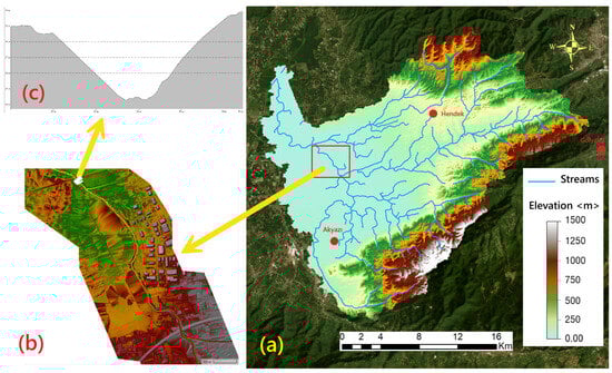
Figure 3.
(a) Digital elevation model (DEM) for HEC-HMS, (b) for HEC-RAS, (c) for river bathymetry.
Then, the effect of rainfall stations on the Dinsiz Stream was calculated using the Thiessen polygon method. Figure 4 shows the rainfall stations and the polygons created based on the Thiessen method.
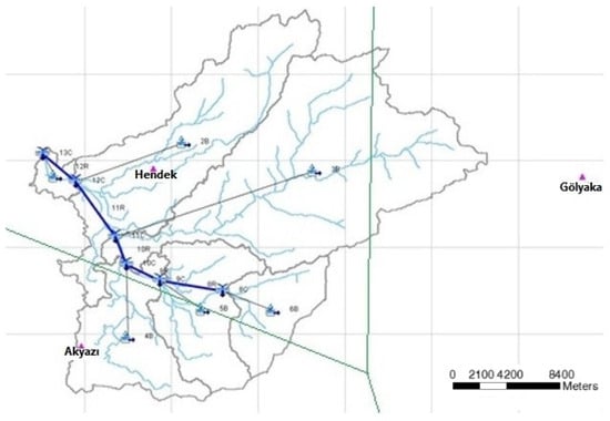
Figure 4.
Basin, sub-basins and rainfall gages in the study area.
In this study, the SCS (Soil Conservation Service) curve number (CN) method, a function of cumulative rainfall, soil cover, land use, and antecedent moisture, was used to calculate rainfall losses. Knowledge of the CN value used in the SCS curve number method is essential for calculating flow values and producing hydrographs during transition from rainfall to flow calculations.
Since it yields acceptable results, the SCS-CN method has been considered a more effective approach for calculating flow volumes [51]. SCS-CN was improved by the United States Department of Agriculture (USDA) and the Natural Resources Conservation Association in the 1950s. CN is determined using parameters such as soil, land use, and hydrological groups. Soil is categorized into four hydrological groups A, B, C, and D, where Group A represents soils with high infiltration rates, and Group D contains soils with low infiltration rates. This method is practical, simple, and provides reliable results, making it widely used [52]. Employing this method, direct flow from rainfall can be calculated approximately, and this technique is accepted for flow estimation in small agricultural basins by the USDA [53]. The SCS-CN model is given in the following Equation (1):
where Q is runoff depth (mm); P is rainfall (mm); Ia is the initial abstraction (mm); S is potential maximum retention (mm) (ability of a basin to abstract and keep storm). Rainfall Ia and S are calculated from the following Equation (2):
The cumulative excess at time t is calculated with Equations (3) and (4).
In this paper, the value of CN for the study location depends on land use, land cover, and hydrological soil group [54]. For basins with sub-basins featuring different land use and land cover, the CN compound value is determined using the CN compound formula Equation (5):
This value could not be obtained from previous studies in this region. Therefore, within the scope of this study, the CN value was manually calculated and assessed with the help of GIS-based programs [55]. The areas were determined by overlapping the hydrological soil group maps and the land use maps produced by the Ministry of Agriculture and Forestry of the Republic of Türkiye for the spring months of 2022, as shown in Figure 5. Then, the units corresponding to these areas (A, B, C, and D) were multiplied by the values in the table of hydrological soil group types. The hydrological soil group map of the location is presented in Figure 6. The calculations were performed, and the CN coefficient was found to be 70.
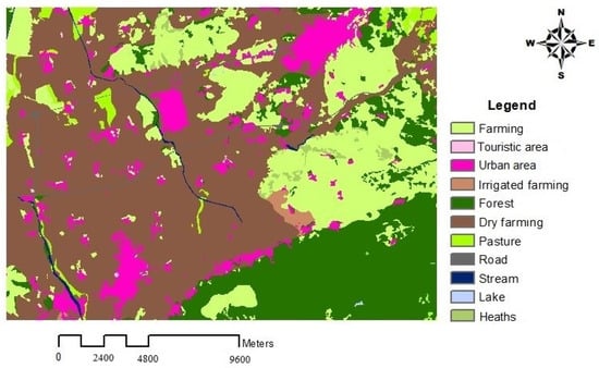
Figure 5.
The land use map of study area.
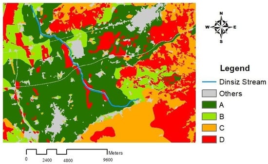
Figure 6.
The hydrologic soil map of the study area.
Subsequently, the calculated CN coefficient and 50, 100, 200, and 500-year annual rainfall values of the stations, shown in Table 3, were added to the program one by one, and four hydrographs were obtained for each sub-basin.
Table 3.
Rainfall return period values (mm) for three stations.
In the HEC-HMS programme, flood hydrographs were obtained from the rainfall values using the SCS type 2 24 h curve given in Figure 7 below. The flood hydrographs obtained from the hydrological model for various return periods are presented in Figure 8.
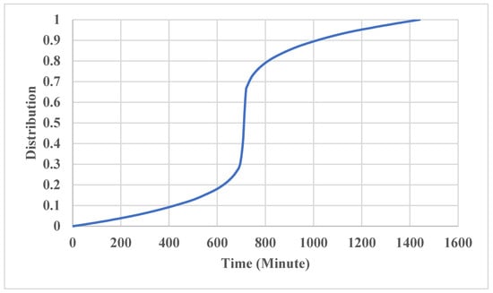
Figure 7.
SCS type II 24 h distribution curve.
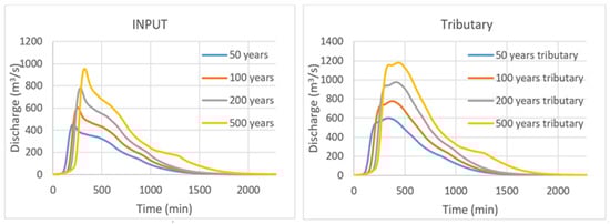
Figure 8.
Flood hydrographs for various return periods.
2.3. Hydraulics Steps
2.3.1. HEC-RAS
In this study, a hydrodynamic model was obtained using HEC-RAS 5.0.7 software. HEC-RAS is a program that performs one- and two-dimensional hydraulic calculations. In addition, it is widely used in various settings such as natural and built canals, floodplain areas, protected areas, etc. [21]. The St Venant equations used in unsteady HEC-RAS 5.0.7 can be expressed as follows:
Equation (6) is defined as the continuity equation, Equation (7) is the x momentum equation, and Equation (8) is the y momentum equation, where u is the x-component of the flow velocity, ν is the y-component of the flow velocity, x and y are the coordinates, h is the cross-sectional mean water depth, n is the manning roughness coefficient, and zb is the bed elevation.
The RAS Mapper and DEM data were used as input in HEC-RAS to create a watershed and geometry. For the two-dimensional flood model of the study area, an area was drawn with the “Geometry” tool; the beginning and end of the Dinsiz Stream formed the boundary conditions.
Obtaining the manning roughness coefficient
The manning coefficient for this study area was calculated using the Cowan method and remote sensing techniques. Field studies were used to evaluate the data used in this method. Originally developed by Cowan [56] (Cowan, 1956), this method was subsequently modified by the US Geological Survey [57]. The parameter n1 was developed by the Turkish State Hydraulic Works [58]. The Cowan method refers to the following equation:
where nb represents the channel’s soil properties, n1 is the side slope type, n2 is the shape and size of the channel, n3 represents the effect of the obstacles in the channel, n4 accounts for flow conditions and the vegetation, and m is the coefficient expressing the degree of curvature of the channel. The coefficients “n” in Equation (9) are provided in the table below [58,59]. In this study, the Manning coefficient used for the river bed in both models (Coupled 1D/2D and 2D) was calculated as 0.0805 according to the Cowan method. The following factors were considered to obtain this value: soil for the river bed, minor channel side slope, occasional change in channel section, noteworthy obstacles in the channel, medium vegetation in the channel and noteworthy channel fold. The corresponding values were obtained using Equation (9).
The selection of parameters used in the Cowan method was made in line with data and observations obtained during the field surveys. Irregularities in the route and bed sections were eliminated in the case investigations within the Dinsiz Stream project. The roughness coefficients were calculated; the roughness coefficients and the assumptions for the projected situation are presented in Table 4. The roughness coefficient was calculated separately for each subsequent kilometer, based on the changes in the coefficient along the improved route during the projected status investigations. It is recommended to use a roughness coefficient of 0.030 for clean and flat land in natural beds, between 0.030–0.035 according to plant density, 0.022 for concrete walls, 0.13 in case of smooth asphalt pavement, 0.016 for rough asphalt, and 0.040 for land consisting of gravel and coarse rocks [60,61].
Table 4.
Modified Cowan method “n” values.
2.3.2. 2D Model
First of all, to create a 2D model, geometry, unsteady flow data, and plan files are required. Subsequently, the terrain data and Manning’s roughness layer must be correlated with the Geometry file [21]. Here, the land use map was used differently from the coupled 1D/2D model. For the defined 2D areas, 10 × 10 was chosen considering the calculation cell size, the accuracy of the model results, and the model runtime. Boundary conditions (input, tributary, and output) were then plotted to add unsteady flow data. The boundary conditions and the 2D model area chosen for this study are illustrated in Figure 9a.
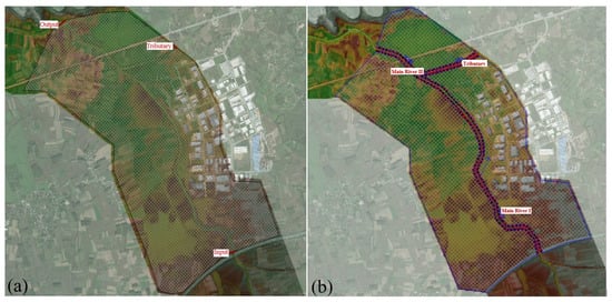
Figure 9.
(a) 2D area and boundary conditions, (b) coupled 1D/2D model area.
2.3.3. Coupled 1D/2D Modelling
The HEC-RAS model can perform 1D, 2D, and coupled 1D/2D simulations. In this case, lateral river structures were used to link the area behind an embankment to couple the 1D and 2D models. The flow over the levee was estimated using the headwater from the 1D river and the tailwater from the 2D flow area. Lateral structures can take the form of a floodwall, levee, or a diversion structure. ersatile and can also represent the flow of a river. In this study, the flow between 1D river reaches and 2D floodplain areas was modelled using the lateral structure tool in HEC-RAS. The following Equations (10) and (11) were used in the HEC-RAS coupled 1D/2D models [62]. Figure 9b shows the coupled 1D/2D model area; the red dashed lines show the connection between the 1D and the 2D models.
In the coupled 1D/2D model within HEC-RAS, the recommended equation for integrating the 1D and 2D models is the weir equation. By default, a “broad-crested weir” type is suggested for the weir equation, and this was adopted in the current study. The coefficient CCC for this type of weir is set to 1 by default, as specified in the program manual.
In this study, both the 1D/2D and 2D models were individually applied to floods with return periods of 50, 100, 200 and 500 years. A total of 8 scenarios were applied, 4 on the 1D/2D model and 4 on the 2D model, and the following results were obtained.
Figure 10 shows the patterns that emerged as a result of this study and the changes in the water levels associated with them. The water level was found to be high in the coupled 1D/2D model results for all four models constructed for possible flood flow rates for 50, 100, 200, and 500-year return periods.
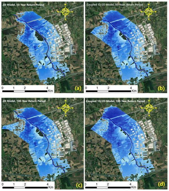
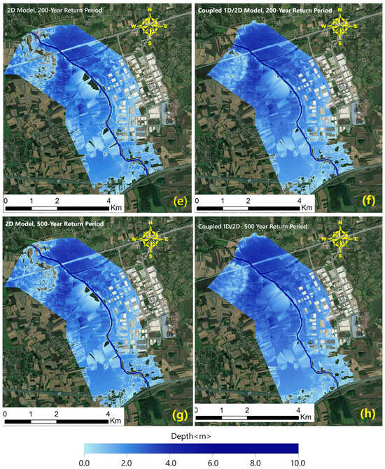
Figure 10.
Flood inundation maps: (a) 50-year 2D model, (b) 50-year 1D/2D coupled model, (c) 100-year 2D model, (d) 100-year 1D/2D coupled model, (e) 200-year 2D model, (f) 200-year 1D/2D coupled model, (g) 500-year 2D model, (h) 500-year 1D/2D coupled model.
Finally, we created an additional model to validate the eight models. The flow data used for this model were obtained from the flood experienced in the region in July 2021. Using the 24 h rainfall values from this flood, a flow hydrograph was constructed and used in the model. The results of this flood event in July 2021 corresponded to a 100-year return period flood flow according to the coupled 1D/2D model and a 500-year return period flood according to the 2D model. This increased the accuracy of the results obtained using these models. Figure 11 shows the hydrograph results of the flood event.
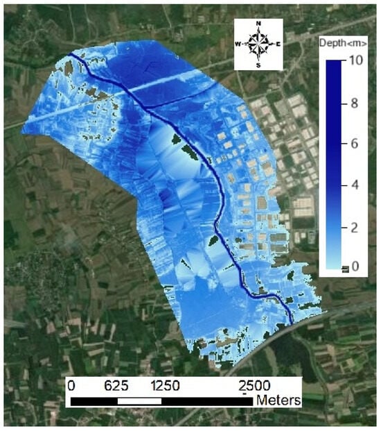
Figure 11.
24 h rainfall peak flow.
3. Results
Located within the boundaries of the Sakarya Basin, the Dinsiz Stream passes through the boundaries of the Hendek and Akyazı districts. Near the stream, there are settlements, agricultural areas, and an organized industrial zone, which is of great economic importance. The potential occurrence of a flood event in this area poses a substantial risk of significant losses.
The Dinsiz Stream, located within the Sakarya Basin, flows through both residential and industrial zones, presenting a significant flood risk. This study aimed to analyze hydrological and hydraulic models using HEC-HMS and HEC-RAS software to evaluate flood propagation under different return periods (50, 100, 200, and 500 years). The findings provide critical insights into flood risk management, particularly by comparing coupled 1D/2D and fully 2D models.
In the coupled 1D/2D models, flood water levels were consistently higher compared with the 2D models across all return periods. This discrepancy was particularly pronounced in the industrial zone, where the water level in the 1D/2D model exceeded that in the 2D model by approximately 1 m (Figure 12). This suggests that the 1D/2D model more accurately captured the interactions between the main river channel and the floodplain, potentially offering a more reliable assessment of flood risks.
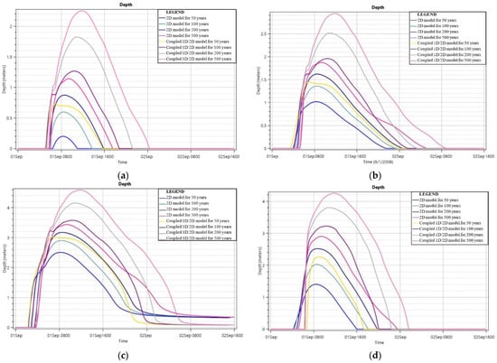
Figure 12.
(a) Depth–time plot of all models for water depth in the flat area, (b) depth–time plot of all models for water depth in the industrial zone, (c) depth–time plot of all models for water depth to the right of tributary, (d) depth–time plot of all models for water depth for a point downstream.
The analysis further revealed that even a 50-year return period flood is sufficient to inundate critical infrastructure, including parts of the second organized industrial zone and surrounding agricultural areas. In particular, the coupled 1D/2D model indicated a more extensive spread of floodwaters, affecting both urban and rural areas. The hydrograph simulations demonstrated a substantial rise in flood levels within the first 8 h of peak rainfall, highlighting the rapid onset of flooding in the region.
Spatial analysis of the flood extent maps revealed that the coupled 1D/2D model predicted a wider inundation area than the 2D model, particularly in low-lying zones and near river confluences. This highlights the model’s ability to incorporate lateral flow interactions, which are often underestimated in purely 2D simulations. Furthermore, a sensitivity analysis was conducted to assess the impact of varying Manning’s roughness coefficients on flood propagation. The results showed that increasing roughness values led to higher flood depths and slower recession times, emphasizing the importance of accurate parameter selection in flood modeling.
Additionally, validation using the July 2021 flood event showed that the coupled 1D/2D model corresponded to a 100-year return period flood, whereas the 2D model produced flood extents comparable to a 500-year return period event. This discrepancy underscores the importance of model selection in flood hazard assessment and mitigation planning.
Finally, a comparative assessment of peak discharge values indicated that the coupled 1D/2D model produced higher peak flows than the 2D model, aligning more closely with observed flood events. This suggests that coupled modeling may offer enhanced predictive capabilities for extreme flood scenarios, providing valuable data for risk mitigation strategies and emergency response planning.
The results of each model revealed that the basin is sensitive to flooding and that the Dinsiz Stream cannot handle the potential flow rates. Thanks to this study, it was determined that the organized industrial zone in the study area is at great risk. Given the high population in the region, there is potential for loss of life. In addition, since there was previously no flood map for the Dinsiz Stream basin, this study addresses a gap in the existing literature.
4. Discussion
The comparative analysis between the coupled 1D/2D and fully 2D modelling approaches demonstrates the advantages and limitations of each method. The coupled 1D/2D model eliminates the need for complex terrain modifications by simulating river flow in 1D while capturing floodplain dynamics in 2D. This hybrid approach can provide more efficient simulations with reduced computational demands. However, setting up and maintaining the interface between the 1D and 2D domains remains a technical challenge, particularly for regions with complex topographies.
In contrast, the fully 2D model offers a more detailed representation of flood behaviour by capturing intricate flow patterns without reliance on predefined cross-sections. This advantage is particularly evident in urban settings where water can disperse in multiple directions. Nonetheless, the higher computational cost and longer processing time may limit its applicability, especially for large-scale flood simulations.
Compared with prior studies, this work provides a unique perspective by directly comparing the results of coupled 1D/2D models with 2D models under identical conditions. While previous research has predominantly focused on calibrating and validating models, this study emphasizes the methodological differences during the model setup process. This distinction is crucial for understanding the trade-offs between accuracy, computation time, and model complexity.
Despite its contributions, this study acknowledges certain limitations. The absence of historical flood data for validation necessitated reliance on visual calibration and hydrological approximations. Additionally, topographic and hydrographic data limitations introduce uncertainties, emphasizing the need for high-resolution DEM datasets in future research. To enhance the accuracy and applicability of flood models, future studies should incorporate advanced remote sensing techniques, sub-grid modelling approaches, and climate change projections.
In the literature, there are very few comparisons of two models similar to the current study. The authors could not establish a connection with previous studies, because the reviewed studies either compared 1D/2D coupled models with 1D models or included only 1D/2D coupled models. Therefore, the authors conducted this current study to attract attention, contribute to the literature, and answer the question of which model would give what results.
5. Conclusions
This study aimed to compare coupled 1D/2D model and 2D model approaches used in different flood scenarios, using HEC-RAS software. In this process, 1D and 2D models were combined to analyse the water levels and flood propagation in flood areas. The novelty of the study is its detailed examination of the results of the two different approaches using the same dataset and modelling environment. The findings provide concrete implications for increasing the efficiency of flood modelling studies. In addition, this research sheds light on the differences between the theoretical performance of 1D/2D models and 2D-only models, which have been overlooked in the literature.
This study has some limitations. Firstly, since historical flood data required for model validation process were not available, the exact accuracy of the model results could not be measured. Instead, the results were theoretically supported by visual calibration and hydraulic modelling approaches. In addition, the topographic and hydrographic data used for modelling the Dinsiz Stream Basin contained some uncertainties due to limited measurement and observation resources. Since high-resolution DEM data should be used for more reliable results, this study was conducted in a limited area. This study does not aim to make a definitive claim about accuracy, but evaluates the methodological differences between the models.
This study provides important implications for flood risk management and urban planning policies. It has been shown that coupled 1D/2D modelling is an effective tool to assess flood propagation faster and at lower cost, especially in regions with limited data resources. This may allow local governments to analyse large flood areas with fewer computational resources. On the other hand, it has been stated that 2D modelling alone can provide more comprehensive outputs in detailed flood analyses. These results may be useful for developing flood mapping strategies, prioritizing at-risk areas, and optimizing disaster management budgets. However, the applicability of the proposed method depends on the local infrastructure and technical capacity.
The maximum difference in water level between the coupled 1D/2D and 2D models was up to 1 m. More research studies on composite models need to be carried out, and their accuracy needs to be discussed further. Flooding poses a great threat to people living in settlements along the stream and to the organized industrial zone. When a flood occurs, more than 1500 residences in the region will be flooded and many workplaces will suffer great financial losses. It is also expected that highway bridges over the stream will be damaged. Dikes should be added along the river banks to restrict flood propagation in the river area. This study should prove informative and exemplary, as similar research has not been carried out previously in the region.
It is clear that the methods presented in this study need to be tested in a broader context. More case studies are needed to compare the performance of 1D/2D combined models and 2D models alone in rural and urban areas. Future research can further accelerate the modelling processes by investigating the applicability of innovative approaches such as sub-grid modelling techniques. In addition, the performance of these models can be tested under different climatic conditions with higher resolution datasets and forward-looking flood scenarios. Improving field data with methods such as remote sensing or drone-based flood observations can increase the accuracy of such models.
Author Contributions
All authors contributed to the preparation and design of this research paper. P.S.: conceptualization, methodology, validation, formal analysis, investigation, resources, visualization, software, writing—original draft. Y.P.: supervision, investigation, visualization, conceptualization. E.D.: review and editing. All authors have read and agreed to the published version of the manuscript.
Funding
This research received no external funding.
Data Availability Statement
The datasets generated and analysed during the current study are available from the corresponding author upon reasonable request.
Acknowledgments
The authors express their gratitude to the Sakarya Meteorology Directorate and the Ministry of Agriculture and Forestry for providing the data used in this study and to the USACE for the programs used. Special thanks are extended to Soner Tuğlu and Abdulbaki Hacı for their assistance in this study.
Conflicts of Interest
The authors declare that they have no known competing financial interests or personal relationships that could have appeared to influence the work reported in this paper.
References
- Kheradmand, S.; Seidou, O.; Konnte, D.; Batoure, M.B.B. Evaluation of adaptation options to flood risk in a probabilistic framework. J. Hydrol. Reg. Stud. 2018, 19, 1–16. [Google Scholar] [CrossRef]
- Munich Reinsurance Company. Natural Loss Events Worldwide 1980–2018 Nat. Cat. Service Munich Reinsurance Company. 2019. Available online: https://natcatservice.munichre.com (accessed on 5 October 2020).
- Azouagh, A.; El Bardai, R.; Hilal, I.; Stitou el Messari, J. Integration of GIS and HEC-RAS in floods modeling of Martil River (Northern Morocco). Eur. Sci. J. 2018, 14, 130. [Google Scholar] [CrossRef]
- Kishore, N.; Marqués, D.; Mahmud, A.; Kiang, M.V.; Rodriguez, I.; Fuller, A.; Ebner, P.; Sorensen, C.; Racy, F.; Lemery, J.; et al. Mortality in Puerto Rico after hurricane Maria. N. Engl. J. Med. 2018, 379, 162–170. [Google Scholar] [CrossRef]
- Malik, A.; Abdalla, R. Geospatial modeling of the impact of sea level rise on coastal communities: Application of Richmond, British Columbia, Canada. Model. Earth Syst. Environ. 2016, 2, 146. [Google Scholar] [CrossRef]
- Shrestha, M.N. Spatially distributed hydrological modelling considering land-use changes using remote sensing and GIS. In Proceedings of the Map Asia Conference, Kuala Lumpur, Malaysia, 13–15 October 2003. [Google Scholar]
- Wheater, H.; Evans, E. Land use, water management and future flood risk. Land Use Policy 2009, 26, 251–264. [Google Scholar] [CrossRef]
- Teng, J.; Jakeman, A.J.; Vaze, J.; Croke, B.F.W.; Dutta, D.; Kim, S. Flood inundation modelling: A review of methods, recent advances and uncertainty analysis. Environ. Model. Softw. 2017, 90, 201–216. [Google Scholar] [CrossRef]
- Quiroga, V.M.; Kure, S.; Udo, K.; Mano, A. Application of 2D numerical simulation for the analysis of the February 2014 Bolivian Amazonia flood: Application of the new HEC-RAS version 5, RIBAGUA. Rev. Iberoam. Agua 2016, 3, 25–33. [Google Scholar] [CrossRef]
- Horritt, M.S. A linearized approach to flow resistance uncertainty in a 2-D finite volume model of flood flow. J. Hydrol. 2002, 316, 13–27. [Google Scholar] [CrossRef]
- Alho, P.; Aaltonen, J. Comparing a 1D hydraulic model with a 2D hydraulic model for the simulation of extreme glacial outburst floods. Hydrol. Process. Int. J. 2008, 22, 1537–1547. [Google Scholar] [CrossRef]
- Leedal, D.; Neal, J.; Beven, K.; Young, P.; Bates, P. Visualization approaches for communicating real-time flood forecasting level and inundation information. J. Flood Risk Manag. 2010, 3, 140–150. [Google Scholar] [CrossRef]
- Vozinaki, A.E.K.; Morianou, G.G.; Alexakis, D.D.; Tsanis, I.K. Comparing 1D and combined 1D/2D hydraulic simulations using high-resolution topographic data: A case study of the Koiliaris basin, Greece. Hydrol. Sci. J. 2017, 62, 642–656. [Google Scholar] [CrossRef]
- Anees, M.T.; Abdullah, K.; Nordin, M.N.M.; Ab Rahman, N.N.N.; Syakir, M.I.; Kadir, M.O.A. One- and Two-dimensional Hydrological Modelling and Their Uncertainties. Flood Risk Manag. 2016, 11, 221–244. [Google Scholar]
- Dutta, D.; Herath, S.; Musiake, K. An application of a flood risk analysis system for impact analysis of a flood control plan in a river basin. Hydrol. Process. 2006, 20, 1365–1384. [Google Scholar] [CrossRef]
- Banks, J.C.; Camp, J.V.; Abkowitz, M.D. Adaptation planning for floods: A review of available tools. Nat. Hazards 2014, 70, 1327–1337. [Google Scholar] [CrossRef]
- DHI. MIKE 21-2D Modelling of Coast and Sea; DHI Water & Environment Pty Ltd.: Hørsholm, Denmark, 2012. [Google Scholar]
- Roberts, S.; Nielsen, O.; Gray, D.; Sexton, J.; Davies, G. ANUGA User Manual; Commonwealth of Australia (Geoscience Australia) and the Australian National University: Canberra, Australia, 2015. [Google Scholar]
- An, H.; Yu, S.; Lee, G.; Ki, Y. Analysis of an open source quadtree grid shallow water solver for flood simulation. Quat. Int. 2015, 384, 118–128. [Google Scholar] [CrossRef]
- An, H.; Yu, S. Well-balanced shallow water flow simulation on quadtree cut cell grids. Adv. Water Resour. 2012, 39, 60–70. [Google Scholar] [CrossRef]
- Brunner, G.W. HEC-RAS River Analysis System Hydraulic Reference Manual Version 5.0. 2016. Available online: https://www.hec.usace.army.mil/software/hec-ras/documentation/HEC-RAS%205.0%20Reference%20Manual.pdf (accessed on 26 September 2021).
- Horritt, M.S.; Bates, P.D. Evaluation of 1D and 2D numerical models for predicting river flood inundation. J. Hydrol. 2002, 268, 87–99. [Google Scholar] [CrossRef]
- Dimitriadis, P.; Tegos, A.; Oikonomou, A.; Pagana, V.; Koukouvinos, A.; Mamassis, N.; Koutsoyiannis, D.; Efstratiadis, A. Comparative evaluation of 1D and quasi-2D hydraulic models based on benchmark and real-world applications for uncertainty assessment in flood mapping. J. Hydrol. 2016, 534, 478–492. [Google Scholar] [CrossRef]
- Bladé, E.; Cea, L.; Coresteina, G.; Escolano, E.; Puertas, J.; Vázquez-Cendón, E.; Dolz, J.; Coll, A. Iber—River modelling simulation tool. Rev. Int. Métodos Numéricos Cálculo Diseño Ing. 2014, 30, 1–10. [Google Scholar] [CrossRef]
- Cook, A.; Merwade, V. Effect of topographic data, geometric configuration and modeling approach on flood inundation mapping. J. Hydrol. 2009, 377, 131–142. [Google Scholar] [CrossRef]
- Neal, J.; Keef, C.; Bates, P.; Beven, K.; Leedal, D. Probabilistic flood risk mapping including spatial dependence. Hydrol. Process. 2012, 27, 1349–1363. [Google Scholar] [CrossRef]
- Sönmez, O.; Doğan, E. Determination of flood inundation area in Cedar River using calibrated and validated 1D and 1D/2D model. Sak. Univ. J. Sci. 2016, 20, 337–347. [Google Scholar] [CrossRef][Green Version]
- Betsholtz, A.; Nordlöf, B. Potentials and Limitations of 1D, 2D and Coupled 1D–2D Flood Modeling in HEC-RAS. Master’s Thesis, Lund University, Lund, Sweden, 2017. [Google Scholar]
- Hammami, S.; Romdhane, H.; Soualmia, A.; Kourta, A. 1D/2D coupling model to assess the impact of dredging works on the Medjerda river floods, Tunisia. J. Mater. Environ. Sci. 2022, 13, 825–839. [Google Scholar]
- Kalra, A.; Joshi, N.; Baral, S.; Pradhan, S.N.; Mambepa, M.; Paudel, S.; Xia, C.; Gupta, R. Coupled 1D and 2D HEC-RAS floodplain modeling of Pecos River in New Mexico. In Proceedings of the 2021 World Environmental and Water Resources Congress, Virtual, 7–11 June 2021; pp. 165–178. [Google Scholar] [CrossRef]
- Dasallas, L.; Kim, Y.; An, H. Case study of HEC-RAS 1D–2D coupling simulation: 2002 Baeksan flood event in Korea. Water 2019, 11, 2048. [Google Scholar] [CrossRef]
- Bates, P.D. Flood inundation prediction. Annu. Rev. Fluid Mech. 2022, 54, 287–315. [Google Scholar] [CrossRef]
- Patel, D.; Ramirez, J.A.; Srivastava, P.K.; Bray, M.; Zhang, S. Assessment of flood inundation mapping of Surat city by coupled 1D/2D hydrodynamic modelling: A case application of the new HEC-RAS 5. Nat. Hazards 2017, 89, 93–130. [Google Scholar] [CrossRef]
- Tazin, T. Flood Hazard Mapping of Dharla River Floodplain Using HEC-RAS 1D/2D Coupled Model. Mater’s Thesis, Bangladesh University of Engineering and Technology (BUET), Dhaka, Bangladesh, 2017. [Google Scholar]
- Rubio, F. Flood Risk Assessment in the Vicinity of Kartena Town Using HEC-RAS 1D–2D Models. Master’s Thesis, Aleksandras Stulginskis University, Kaunas, Lithuania, 2018. [Google Scholar]
- Ucar, I.; Kapcak, M.; Sonmez, O.; Dogan, E.; Turan, B.; Dal, M.; Findik, S.B.; Yilmaz, M.; Sever, A. From Hazard Maps to Action Plans: Comprehensive Flood Risk Mitigation in the Susurluk Basin. Water 2025, 17, 860. [Google Scholar] [CrossRef]
- Kulkarni, A.D.; Kale, G.D. The Development of Coupled 1D–2D Hydrodynamic Flood Model by Using HEC-RAS: A Case Study of the Panchganga River Basin, Kolhapur District, Maharashtra, India. Water Resour. 2024, 51, 789–799. [Google Scholar] [CrossRef]
- Siakara, G.; Gourgouletis, N.; Baltas, E. Assessing the Efficiency of Fully Two-Dimensional Hydraulic HEC-RAS Models in Rivers of Cyprus. Geographies 2024, 4, 513–536. [Google Scholar] [CrossRef]
- Lim, M.; Ginting, B.M.; Senjaya, T.; Kieswant, C. Comparison of 1D, coupled 1D–2D, and 2D shallow water numerical modeling for dam-break flow analysis of Way-Ela dam, Indonesia. Acta Hydrotech. 2024, 37, 27–50. [Google Scholar] [CrossRef]
- Moghim, S.; Gharehtoragh, M.A.; Safaie, A. Performance of the flood models in different topographies. J. Hydrol. 2023, 620, 129446. [Google Scholar] [CrossRef]
- Özcan, O. Determination of Flood Risk Analysis of Sakarya River Sub-Basin with Remote Sensing and CBS. Master’s Thesis, Istanbul Technical University, Istanbul, Turkey, 2008. [Google Scholar]
- Koliokosta, E. Return Periods in Assessing Climate Change Risks: Uses and Misuses. Environ. Sci. Proc. 2023, 26, 75. [Google Scholar] [CrossRef]
- Van Campenhout, J.; Houbrechts, G.; Peeters, A.; Petit, F. Return Period of Characteristic Discharges from the Comparison between Partial Duration and Annual Series, Application to the Walloon Rivers (Belgium). Water 2020, 12, 792. [Google Scholar] [CrossRef]
- Di Baldassarre, G.; Montanari, A.; Lins, H.; Koutsoyiannis, D.; Brandimarte, L.; Blöschl, G. Flood fatalities in Africa: From diagnosis to mitigation. Geophys. Res. Lett. 2010, 37, L22402. [Google Scholar] [CrossRef]
- Jobe, A.; Bhandari, S.; Kalra, A.; Ahmad, S. Ice-Cover and jamming effects on inline structures and upstream water levels. In Proceedings of the 2017 World Environmental and Water Resources Congress, Sacramento, CA, USA, 21–25 May 2017; pp. 270–279. [Google Scholar] [CrossRef]
- Sagarika, S.; Kalra, A.; Ahmad, S. Interconnections between oceanic-atmospheric indices and variability in the U.S. streamflow. J. Hydrol. 2015, 525, 724–736. [Google Scholar] [CrossRef]
- Sagarika, S.; Kalra, A.; Ahmad, S. Pacific Ocean SST and Z500 climate variability and western U.S. seasonal streamflow. Int. J. Climatol. 2016, 36, 1515–1533. [Google Scholar] [CrossRef]
- United States Army Crops of Engineers (USACE). HEC-HMS Hydrologic Modelling System User’s Manual; Hydrologic Engineering Center: Davis, CA, USA, 2001.
- Feldman, A.D. Hydrologic Modelling System HEC-HMS Technical Reference Manual; CDP-74B; US Army Corps of Engineers: Washington, DC, USA, 2000.
- Scharffenberg, W.; Ely, P.; Daly, S.; Fleming, M.; Pak, J. Hydrologic modelling system (HEC-HMS): Physically-based simulation components. In Proceedings of the 2nd Joint Federal Interagency Conference, Las Vegas, NV, USA, 27 June–1 July 2010. [Google Scholar]
- Schulze, R.E.; Schmidt, E.J.; Smithers, J.C. SCS-SA User Manual PC Based SCS Design Flood Estimates for Small Catchments in Southern Africa; Department of Agricultural Engineering, University of Natal: Pietermaritzburg, South Africa, 1992. [Google Scholar]
- Katara, P.; Machiwal, D.; Mittal, H.K.; Dashora, Y.; Bhagat, A. Estimation of Runoff for Ahar River Catchment in Udaipur District. Integrated Remote Sensing and Geographical Information System; The Institute of Engineers (India) Udaipur Local Centre: Udaipur, India, 2013; pp. 169–175. [Google Scholar]
- United States Department of Agriculture (USDA). Estimation of direct runoff from storm rainfall, Part 630 Hydrology. In National Engineering Handbook; United States Department of Agriculture (USDA): Washington, DC, USA, 2004. [Google Scholar]
- Soil Conservation Service. Hydrology, National Engineering Handbook; Soil Conservation Service, USDA: Washington, DC, USA, 1985.
- Zhan, X.; Huang, M.L. ArcCN-Runoff: An ArcGIS tool for generating curve number and runoff maps. Environ. Model. Softw. 2004, 19, 875–879. [Google Scholar] [CrossRef]
- Cowan, W.L. Estimating hydraulic roughness coefficients. Agric. Eng. 1956, 37, 473–475. [Google Scholar]
- Arcement, G.J.; Schneider, V.R. Guide for Selecting Manning’s Roughness Coefficients for Natural Channels and Flood Plains, Final Repo; U.S. Department of Transportation: Washington, DC, USA, 1984.
- Turkish State Hydraulic Works (DSI). Roughness Coefficient Determination Guide for Stream Beds; Ministry of Forestry and Water Affairs, General Directorate of State Hydraulic Works: Ankara, Turkey, 2016.
- Barnes, H.H. Roughness Characteristics of Natural Channels; Technical Report; U.S. Geological Survey Water-Supply; United States Government Printing Office: Washington, DC, USA, 1987.
- Chow, V.T. Open Channel Hydraulics; McGraw-Hill: New York, NY, USA, 1959. [Google Scholar]
- Nas, S.S.; Nas, E. Determination of flood areas with the help of geographic information systems and risk analysis: The example of Harşit Stream (Gümüşhane). In Proceedings of the Flood and Landslide, Trabzon, Türkiye, 24–26 October 2013. [Google Scholar]
- Brunner, G.W. Creating and Combined 1D/2D Model; US Army Corps of Engineers, Institute for Water Resources, Hydrologic Engineering Center: Davis, CA, USA, 2016. Available online: https://www.hec.usace.army.mil/confluence/rasdocs/hgt/latest/guides/creating-an-combined-1d-2d-model (accessed on 26 September 2021).


Disclaimer/Publisher’s Note: The statements, opinions and data contained in all publications are solely those of the individual author(s) and contributor(s) and not of MDPI and/or the editor(s). MDPI and/or the editor(s) disclaim responsibility for any injury to people or property resulting from any ideas, methods, instructions or products referred to in the content. |
© 2025 by the authors. Licensee MDPI, Basel, Switzerland. This article is an open access article distributed under the terms and conditions of the Creative Commons Attribution (CC BY) license (https://creativecommons.org/licenses/by/4.0/).