Abstract
The parameters of Low-Impact Development (LID) facilities significantly influence their operational performance and runoff control effectiveness at the site. Despite extensive research on LID effectiveness, limited studies have focused on optimizing design parameters at a community-wide scale, integrating both hydrological and statistical methodologies. A novel approach to optimizing LID design parameters was presented in this study. This study established a community-scale SWMM model, identified the key parameters by the Morris screening method, and determined the reasonable parameter ranges based on runoff control effects. The Response Surface Methodology (RSM) was applied to optimize the key parameters under different return periods and impervious area ratios. The results showed that key LID parameters for runoff volume control were the berm height of the surface layer of sunken greenbelt (SG_Surface_H), the conductivity of the soil layer of sunken greenbelt (SG_Soil_I), the permeability of the pavement layer of permeable pavement (PP_Pavement_I), and the thickness of the storage layer of permeable pavement (PP_Storage_T). The reasonable ranges were 50–265 mm, 5–80 mm/h, 50–140 mm/h, and 100–165 mm, respectively. The key LID parameters for peak flow reduction were SG_Surface_H, SG_Soil_I, PP_Pavement_I, and the berm height of the surface layer of vegetated swale (VS_Surface_H). The reasonable ranges were 50–260 mm, 5–50 mm/h, 50–195 mm/h, and 50–145 mm, respectively. The optimization results of LID parameters showed that for the runoff volume control rate, the optimization strategy involved increasing SG_Surface_H as the return period increased and when the impervious area ratio was large, especially in the rehabilitation of old communities. Meanwhile, the optimal value of SG_Soil_I for runoff volume control was greater than that for peak flow reduction. In contrast, the optimal value of PP_Pavement_I was larger for peak flow reduction. This study provides a significant reference for LID planning and design by emphasizing the optimization of LID design parameters.
1. Introduction
Rapid urbanization has led to the expansion of urban impervious surfaces, resulting in a series of hydrological and environmental issues, such as significantly increased surface runoff, reduced rainwater infiltration, frequent urban flooding, and non-point source pollution [1]. In response to these challenges, China has been actively promoting and implementing the advanced concepts and technologies of sponge city construction across the country. The overarching goal is to reinstate the original natural hydrological conditions that prevailed prior to urban development [2]. Low-Impact Development (LID) technology constitutes a crucial component of the “source-midway-end” integrated technology system in sponge city construction [1]. It places great emphasis on decentralized runoff control at the source. It effectively controls runoff volume, reduces peak flow, mitigates non-point source pollution, and contributes to addressing climate change [3,4]. The main technical facilities of LID technology include green roof, permeable pavement, bioretention cell, rain garden, sunken greenbelt, and vegetated swale. Faced with a variety of design parameters for different facilities, it is worth looking at how to optimize the design of LID parameters so that each LID facility fully plays its role in improving the runoff control effect at the construction site.
Current research has focused on the runoff volume and pollution control effectiveness of individual and combined LID facilities through experimentation, monitoring, and simulation [5,6,7,8,9,10]. However, there are fewer studies on the effects of specific LID parameters on runoff control in actual engineering projects. Guerra and Kim [11] analyzed the applicability of LID structures under varying soil infiltration conditions, recommending a medium depth of 0.4–1.0 m and a maximum infiltration rate of 200 mm/h. In order to fully realize the synergistic effect of various facilities and achieve multi-objective control, optimizing the types, layout, and scale of LID facilities is an important research direction. Existing studies commonly use a combination of hydrological models and genetic algorithms to achieve multi-objective optimization [12,13,14,15,16]. However, relatively few studies have explored the optimization of LID parameters using this method. Lopes and da Silva [17] optimized the areas of the LIDs and the thickness of their storage and soil layer using a simulation–optimization approach based on the SWMM model and the Genetic Algorithm NSGA-II. Zhu et al. [18] optimized the spatial layout and the structural parameters of LIDs under different runoff processes, using the SWMM model combined with the model-independent parameter estimation (PEST). It is worth pointing out that although automating the optimization of LID parameters by integrating genetic algorithms with hydrologic modeling is feasible, this approach has certain limitations, such as the large quantity of LID parameters, the programming expertise required, and the computational efficiency.
The Response Surface Methodology (RSM) serves as an optimization method for comprehensive experimental design and mathematical modeling [19]. As pointed out by Chelladurai et al. [20], the RSM is distinguished by its ability to achieve high-precision outcomes with a relatively small number of experiments and has been extensively applied in fields such as chemistry, environmental science, and food technology. During the planning and design phase of LID, a multitude of parameters must be considered, many of which exhibit complex interactions that influence runoff control performance. The traditional one-variable-at-a-time approach has several drawbacks, including the requirement for a large number of experiments, which is time-consuming and inefficient, as well as its inability to account for the interaction effects among variables. By employing statistical and mathematical modeling approaches, the RSM can effectively reduce the number of runs of the SWMM model. The RSM can explicitly establish the relationships between various input LID parameters and the output response indicators of runoff volume control. Even for complex nonlinear systems, the RSM is capable of identifying optimal parameter combinations. Therefore, the RSM serves as an effective tool for optimizing LID design.
Design Expert software (version 8.0.6) has the capabilities for RSM optimization analysis. It is used for statistical analysis, curve fitting, mathematical modeling, and experimental optimization. It has been widely used in multi-factor experimental design and analysis [21]. Design Expert software can efficiently analyze quadratic polynomial equations and conduct surface analysis using the RSM. Additionally, its user-friendly interface allows us to obtain automatic optimization results from response surface analysis. Li et al. [22] used the DRAINMOD model and RSM to demonstrate that the optimal minimum thickness of the substrate layer of the rain garden was 37 cm, with a maximum thickness of 80 cm, while the optimal depth of the submerged area was at least 22 cm, reaching a maximum of 45 cm. Li et al. [23] optimized the design parameters of bioretention facilities using the HYDRUS-1D model and RSM, with the results showing that the thickness of the medium layer ranged from 25 cm to 120 cm under a high influent concentration. These studies mainly focused on the runoff control effects of a single LID facility, but the parameter optimization of multiple facilities at the community scale requires further intensive research.
Considering the shortcomings in previous studies regarding the impacts of LID parameters on the effectiveness of runoff control and the optimization of LID parameter values, the objectives of this study are as follows: (1) to identify the key parameters of LID facilities that significantly impact the runoff control effects in the study area; (2) to determine the reasonable ranges for the key parameters of LID facilities based on different runoff control objectives; and (3) to optimize the values of the key parameters of LID facilities under different scenarios. This study proposes an optimization analysis approach for LID facility parameters at the community scale using the RSM, providing a scientific foundation for the rational design of LID facilities and maximizing their effectiveness.
2. Materials and Methods
The overall framework for optimizing LID parameters is described in Figure 1. In the first step, the SWMM model is established, and it is calibrated and validated using observed rainfall and flow data. In the second step, the sensitivity analysis of LID parameters is carried out using the Morris screening method to identify key LID parameters and reduce the number of parameters for further analysis. Meanwhile, the ranges of key LID parameters are narrowed by evaluating their effects on runoff volume control and peak flow reduction. In the third step, LID parameters are optimized using the RSM based on the identified ranges of key parameters, considering different rainfall scenarios and impervious area scenarios.
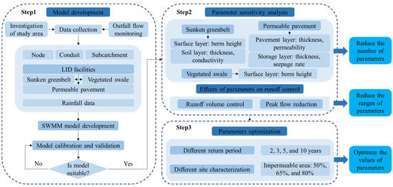
Figure 1.
Optimization framework for LID parameters.
2.1. Study Area
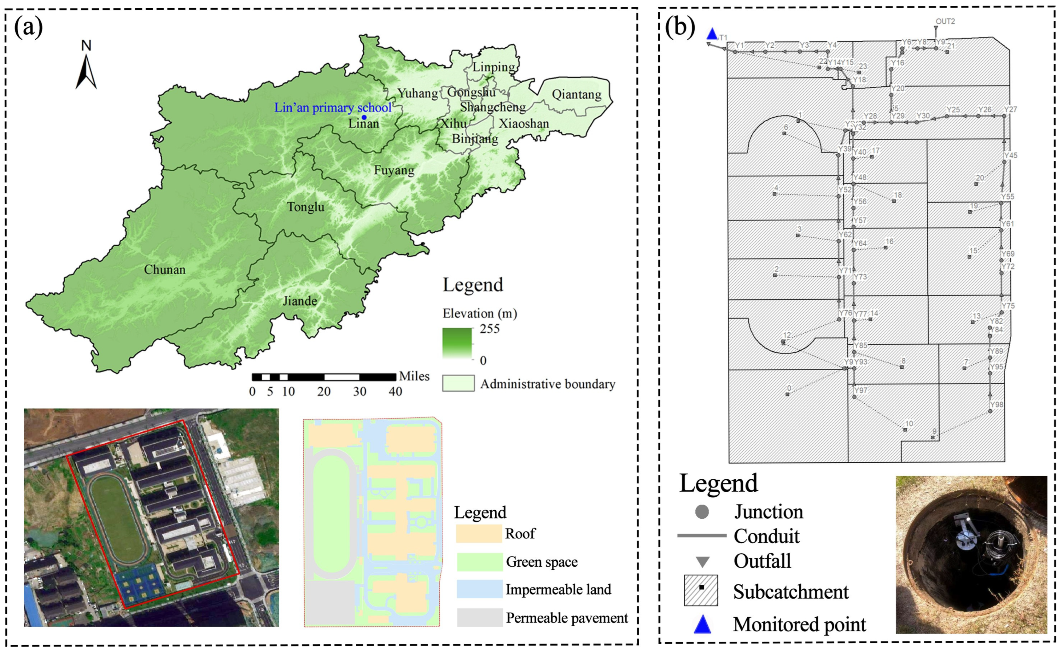
The study area is located in the Lin’an District of Hangzhou, Zhejiang Province, China (Figure 2a). The region experiences a subtropical monsoon climate with an average annual temperature of 17.8 °C. The rainy reason mainly occurs from May to September with an average annual rainfall of 1453 mm. The study area is a sponge city construction project covering a total area of 3.31 ha. The land use type is a primary school with an impervious surface ratio of 65.3% (Figure 2a). LID facilities have been established, encompassing the sunken greenbelt (SG) with an area of 1847 m2, vegetated swale (VS) with a length of 253 m, and permeable pavement (PP) covering an area of 6691 m2.
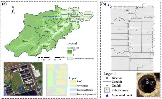
Figure 2.
(a) Location and the underlying surface of the study area; (b) SWMM model of the study area and the monitoring equipment.
The process of urbanization has led to a significant increase in impervious surfaces. During the rainy season, Hangzhou, like many other cities in China, faces challenges such as increased runoff volume, urban waterlogging, and non-point source pollution. Hangzhou is a national-level demonstration city for sponge city construction in China, and the study area is a key stormwater management project in Lin’an District, which is highly representative of urban hydrological challenges. Additionally, abundant data, including online flow monitoring data, have supported the development of the SWMM model for the study area. The findings of this study can provide valuable insights for the rational planning and design of LID at the community scale in China.
2.2. SWMM Model Development
2.2.1. Model Setup
SWMM, developed by the United States Environmental Protection Agency (USEPA), was used to simulate the runoff in this study. As an open-source software, SWMM has been widely applied in LID design and optimization, drainage system design, and the evaluation of runoff control effectiveness [17,18,24,25,26]. The SWMM model of the study area included 24 sub-catchments, 49 manholes, 49 pipes, and 2 outfalls (Figure 2b). Sub-catchments were delineated based on the layout of the drainage network and the flow paths from different types of surfaces to the drainage system. The Horton model was selected for simulating the infiltration process [27]. The Dynamic Wave model was chosen to simulate the hydraulic calculations. The geometric attributes of junctions, outfalls, and conduits were extracted from CAD drawings of the drainage systems. The area, slope, and impervious surface ratio of the sub-catchments were derived from the ArcGIS maps of the generalized sub-catchments. The characteristic width of the sub-catchments was calculated by Equation (1), which provides an efficient estimation without calculating the flow path length of each sub-catchment [17]. Krebs et al. [28] found that the values of k for most of the 2652 sub-catchments ranged from 0.5 to 1.1, with the majority concentrated at 0.7. Therefore, a k-value of 0.7 was selected for this study. Meanwhile, uncertain parameters of the sub-catchments, such as the infiltration coefficient, Manning’s roughness coefficient of impervious and pervious areas, and the depression storage capacity of impervious and pervious areas, need to be manually adjusted through model calibration and validation.
where is the characteristic width, is a dimensionless coefficient, and is the sub-catchment area.
2.2.2. Calibration and Validation Criteria
The Nash-Sutcliffe efficiency (NSE) was used for parameter calibration and validation of the SWMM model [29]. The NSE serves as an indicator of the degree of agreement between the simulated results and observed data (Equation (2)). According to “Assessment Standard for Sponge City Construction Effect” [30], the NSE should not be less than 0.5. In this study, the monitored flow data were obtained from the monitoring point (Out1) (Figure 2b). Flow data were collected in real time using a Doppler flow meter and recorded at 5 min intervals. Due to the limited amount of effective monitoring data, this study used two rainfall events for model calibration and validation. The rainfall event on 8 June 2023, with a rainfall amount of 5.6 mm and a duration of 3.4 h, was used for model calibration. This type of small rainfall event is representative, as small rainfall events (p < 10 mm) account for a significant proportion of precipitation in the study area. Therefore, the calibration results effectively reflected the model’s performance under normal hydrological conditions. The rainfall event on 23 June 2023, with a rainfall amount of 88.3 mm and a duration of 45.5 h, was used for model validation. This extreme rainfall event was selected to assess the model’s performance under special rainfall conditions and to evaluate its adaptability across a wide range of hydrological conditions.
where is the observed value at time t, is the simulated value at time t, and is the average of the observed values.
2.3. Implementing Scenarios
2.3.1. Rainfall Scenario Setting
The rainfall was designed using the storm intensity formula of Lin’an District to simulate rainfall events under different return periods (Equation (3)). In this study, rainfall time series for 2-year, 3-year, 5-year, and 10-year return periods were established based on the Chicago rainfall pattern. The rain peak is 0.4, and the rainfall duration is 2 h [18,24]. Meanwhile, the simulation duration was extended to 5 h to account for the response time of the drainage system and to reflect the complete hydrological process. These four rainfall scenarios were employed for subsequent sensitivity analysis and optimization of LID parameters.
where is the rainfall intensity [L/(s·ha)], is the return period (a), and is the rainfall duration (min).
2.3.2. Impervious Area Scenario Setting
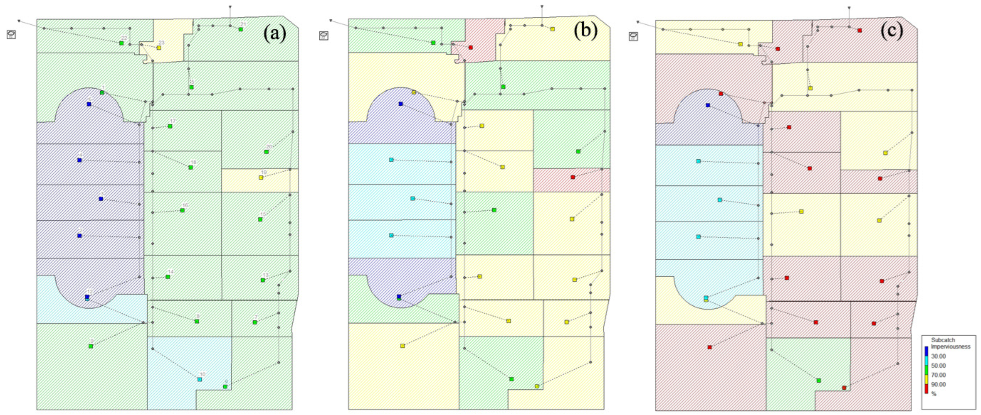
The hydrological impacts of urbanization are primarily driven by the increase in impervious surfaces [31,32]. In addition to the rainfall scenario, various impervious area scenarios were established to investigate the effects of different impervious area ratios on the optimization of LID parameters under the return periods of 3a. The existing model, after the model calibration, was used as a basic scenario. Based on the existing impervious area ratio of approximately 65%, the overall impervious area ratio of the study area was increased to 85% and decreased to 50% by uniformly modifying the impervious area of each sub-catchment in the SWMM model (Figure 3). The impervious area ratio was adjusted by conversion between the areas of green spaces and impervious surfaces.
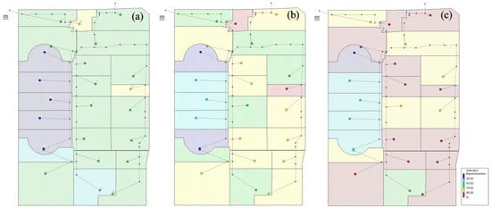
Figure 3.
Different impervious area ratios of the study area: (a) 50%; (b) 65%; (c) 80%.
2.4. Sensitivity Analysis Method
Parameter sensitivity analysis can select high-impact LID parameters in the SWMM model. The Morris screening method, which is a global sensitivity analysis technique based on the one-factor-at-a-time principle, was used to analyze the sensitivity of parameters [33]. Individual parameters were perturbed with a fixed step size of 10%, while others remained constant. In this study, the perturbation ranges for LID parameters were set from −80% to +80% of each initial value [34]. The values of the actual parameters in the calibrated model were employed as the initial values. Meanwhile, the perturbation results of LID parameters should not exceed the specified range of each parameter (Table 1). The sensitivity coefficient (S) is commonly adopted as a criterion for parameter sensitivity [35], as shown in Equation (4). The classification levels are as follows [36]: 0 ≤ |S| < 0.05 means insensitive parameters, 0.05 ≤ |S| < 0.2 means moderately sensitive parameters, 0.2 ≤ |S| < 1 means sensitive parameters, and |S| ≥ 1 means highly sensitive parameters.
where is the sensitivity coefficient, and are the output results after the model of and run, respectively; is the initial output result of the model, and are the change percentages of the parameter value relative to the initial value at the model of and run, respectively (%); and is the number of model operations.

Table 1.
Perturbation results of LID parameters for the SWMM model. SG: sunken greenbelt; VS: vegetative swale; PP: permeable pavement.
Retention and infiltration serve as the dominant hydrologic processes. Therefore, the LID parameters used for sensitivity analysis in this study focused mainly on retention and infiltration related parameters (Table 1). Figure 4 displays schematic diagrams of LID facility structures. Specifically, the parameters of the sunken greenbelt were the berm height of the surface layer (SG_Surface_H), the thickness of the soil layer (SG_Soil_T), and the conductivity of the soil layer (SG_Soil_I). The parameter of the vegetated swale was the berm height of the surface layer (VS_Surface_H). The parameters of the permeable pavement were the thickness of the pavement layer (PP_Pavement_T), the permeability of the pavement layer (PP_Pavement_I), the thickness of the storage layer (PP_Storage_T), and the seepage rate of the storage layer (PP_Storage_I). These LID parameters were utilized in the Morris screening method to assess the extent to which the model was affected. In this study, two key runoff control indicators of the model results were selected, including the runoff volume control rate and the peak flow reduction rate, as shown in Equations (5) and (6). Moreover, parameter sensitivity analysis was carried out under various return periods.
where is the rainfall for each return period (m3), is the runoff volume of the model for each change in LID parameters (m3), is the peak flow before the implementation of LID (m3/s), and is the peak flow of the model for each change in LID parameters (m3/s).
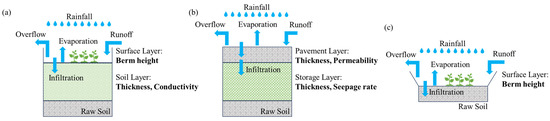
Figure 4.
Schematic diagrams of LID facilities: (a) sunken greenbelt; (b) permeable pavement; (c) vegetated swale.
2.5. Response Surface Methodology
The Response Surface Methodology (RSM) was applied for the optimization analysis of LID parameters with Design Expert Software 8.0.6. RSM is a statistical method used to assist in finding the effects of factors on response variables, reducing the number of experiments, and optimizing each factor [37,38]. In this study, a four-factor, three-level Box–Behnken Design was employed to determine the combination of the LID parameters. The four factors for runoff volume control were SG_Surface_H (A), SG_Soil_I (B), PP_Pavement_I (C), and PP_Storage_T (D), while the four factors for peak flow reduction were SG_Surface_H (A), SG_Soil_I (B), VS_Surface_H (C), and PP_Pavement_I (D) (Section 3.2). The optimization analysis ranges of LID parameters are detailed in Section 3.3. The runoff volume control rate and peak flow reduction rate were selected as response variables. There were 24 different combined coded levels and 3 central coded levels for each response variable, as shown in Table 2. The reliability of the analysis results was evaluated based on various statistical parameters, such as the F-value, p-value, Adequate Precision (AP), R2, Adj R2, and Pred R2.
Table 2.
RSM model experimental design under different runoff control objectives.
3. Results and Discussion
3.1. SWMM Model Calibration and Validation
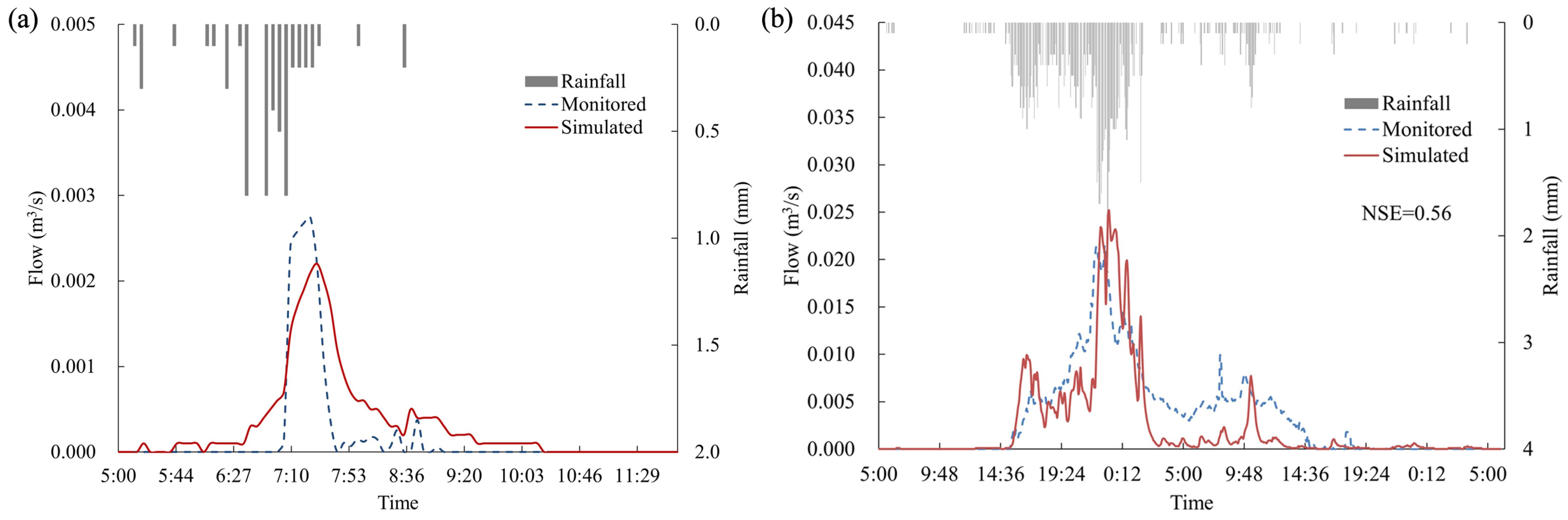
The calibration and validation results of the SWMM model indicated acceptable prediction accuracy (Figure 5). The NSE values were 0.63 and 0.56, respectively. While the approach of using rainfall events of different magnitudes for model calibration and validation allowed for a comprehensive evaluation of the model’s applicability across a wide range of hydrological conditions, it also introduced some limitations. During the calibration phase, the simulated peak flow was slightly lower than the monitored value, whereas during the validation phase, it exceeded the monitored value. These discrepancies underscored the complexities associated with modeling hydrological processes under varying rainfall intensities and durations. Conducting long-term monitoring is essential for improving the accuracy of model predictions in the future. A summary of the calibrated hydrological and hydraulic parameters of the SWMM model is presented in Table 3.
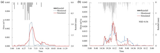
Figure 5.
Results of model calibration (a) and validation (b).
Table 3.
The calibrated hydrologic and hydraulic parameters of SWMM.
3.2. Parameter Sensitivity Analysis
Overall, to comprehensively analyze the impacts of LID parameters on runoff control, four key LID parameters were identified for runoff volume control: SG_Surface_H, SG_Soil_I, PP_Pavement_I, and PP_Storage_T. Similarly, four key LID parameters were identified for peak flow reduction: SG_Surface_H, SG_Soil_I, VS_Surface_H, and PP_Pavement_I (Table 4). According to [22,23], the parameters related to the storage depth, the thickness of soil layer, and the infiltration rate of the rain garden and bioretention facility were sensitive to runoff volume control. In this study, SG_Surface_H, SG_Soil_I, and PP_Pavement_I exhibited varying degrees of sensitivity to both runoff volume control and peak flow reduction. Among them, SG_Surface_H displayed the highest sensitivity. Additionally, PP_Storage_T was sensitive only to runoff volume control, while VS_Surface_H was sensitive only to peak flow reduction. Meanwhile, the sensitivity of LID parameters to runoff volume control and peak flow reduction generally increased as the return period increased, except for PP_Pavement_I, which showed no change for runoff volume control. Similarly to the findings in Zhuang et al. [25], the highly sensitive LID parameters they found in a dense community with a 50-year return period included conductivity of the soil layer of bioretention and the seepage rate of the storage layer of permeable pavement for total runoff control, as well as the conductivity of the bioretention’s soil layer, pavement permeability and the storage seepage rate of the permeable pavement for peak runoff control.
Table 4.
Sensitivity analysis of LID parameters under different return periods for runoff volume control and peak flow reduction.
3.3. Effects of LID Parameters on Runoff Control
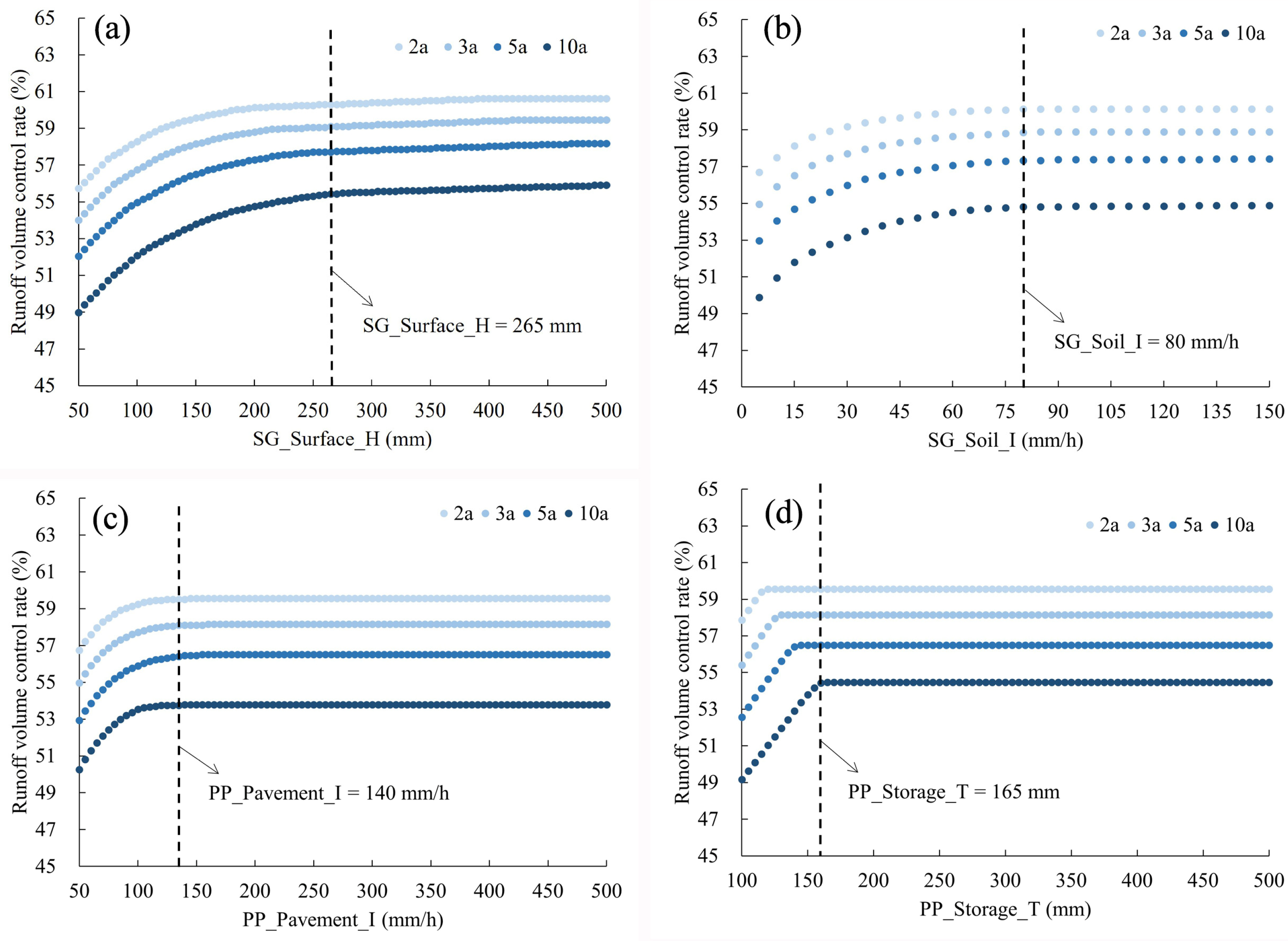
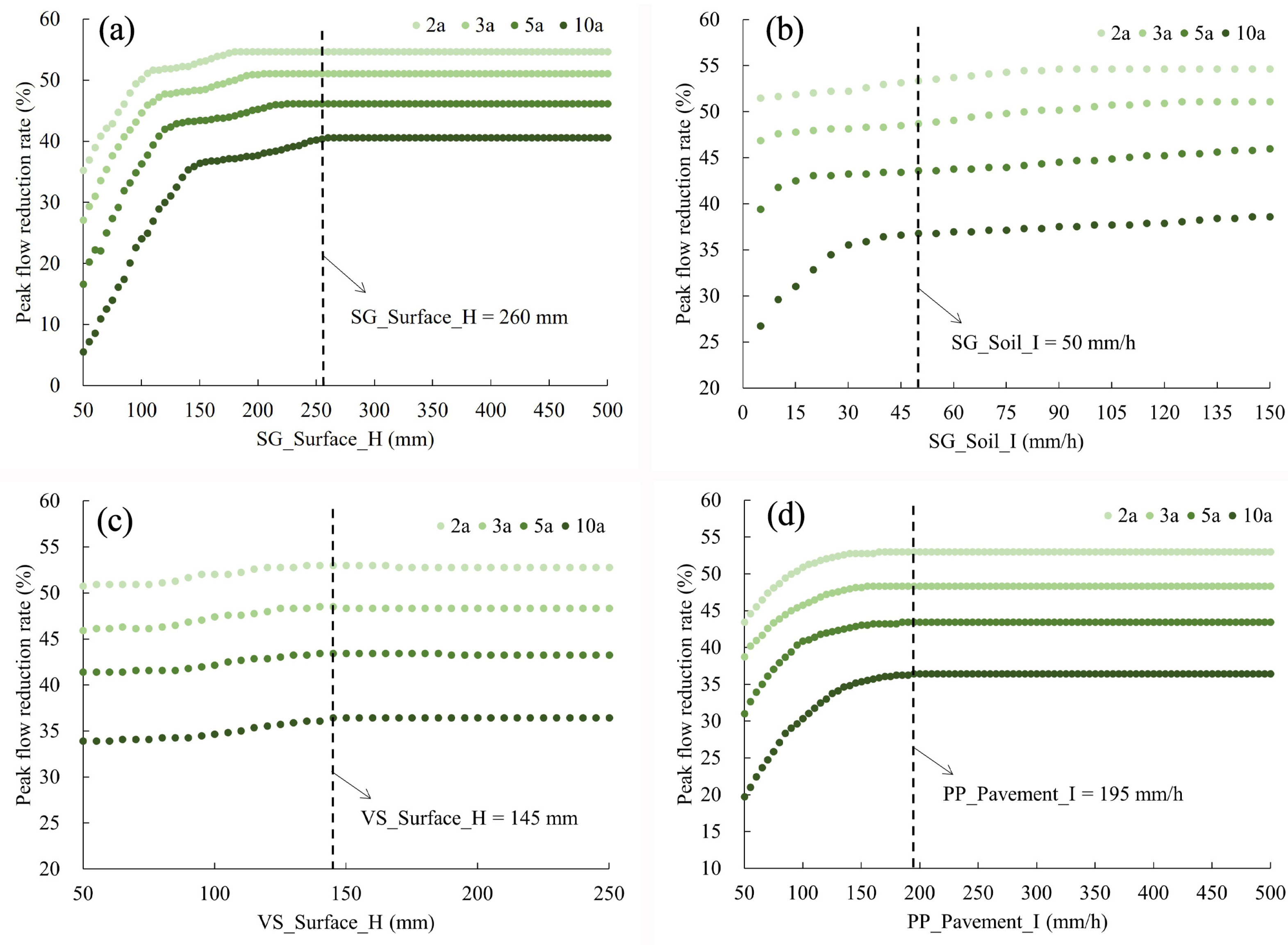
Based on the simulation results from the parameter sensitivity analysis, the effects of key LID parameters on runoff volume control and peak flow reduction were analyzed (Figure 6 and Figure 7). Each data point in the figures represents the result of a single simulation corresponding to each change in LID parameters. When the LID parameters were fixed, the effectiveness of runoff volume control and peak flow reduction gradually decreased as the return period increased. The runoff volume control rate and peak flow reduction rate gradually increased and then leveled out with increasing LID parameters. In this study, the ranges of variation in the runoff volume control rate and peak flow reduction rate were most affected by SG_Surface_H, which was consistent with results of sensitivity analysis. As with the findings of Davis et al. [39], the Bioretention Abstraction Volume (BAV) was directly related to storage in the surface bowl. For example, under the return period of 3a, the effects of SG_Surface_H, SG_Soil_I, PP_Pavement_I, and PP_Storage_T on the runoff volume control rate ranged from 54.0% to 59.5%, 55.0% to 58.9%, 55.0% to 58.2%, and 55.4% to 58.2%, respectively. The effects of SG_Surface_H, SG_Soil_I, PP_Pavement_I, and VS_Surface_H on peak flow reduction rate ranged from 27.1% to 51.1%, 46.9% to 51.1%, 38.7% to 48.3%, and 45.9% to 48.3%, respectively.
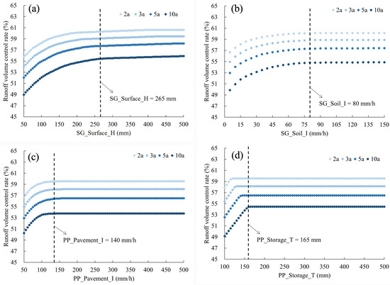
Figure 6.
Effects of LID parameters on runoff volume control rate under different return periods: (a) SG_Surface_H; (b) SG_Soil_I; (c) PP_Pavement_I; (d) PP_Storage_T.
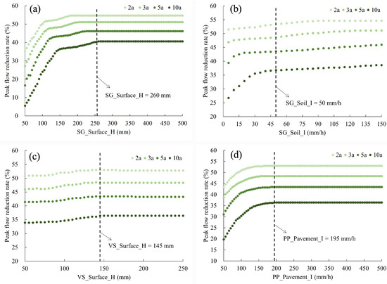
Figure 7.
Effects of LID parameters on peak flow reduction rate under different return periods: (a) SG_Surface_H; (b) SG_Soil_I; (c) VS_Surface_H; (d) PP_Pavement_I.
The thresholds of LID parameters were identified based on the changes in the slope of the curve and the phenomenon that the runoff control effects remained essentially unchanged during the final stage. Then, the reasonable ranges for the optimization analysis of LID parameters were determined for future RSM analysis (Figure 6 and Figure 7). The optimization analysis ranges of SG_Surface_H, SG_Soil_I, PP_Pavement_I, and PP_Storage_T for runoff volume control were 50–265 mm, 5–80 mm/h, 50–140 mm/h, and 100–165 mm, respectively. The optimization analysis ranges of SG_Surface_H, SG_Soil_I, VS_Surface_H, and PP_Pavement_I for runoff volume control were 50–260 mm, 5–50 mm/h, 50–145 mm, and 50–195 mm/h, respectively.
3.4. Statistical Analysis for RSM Models
The F-value and p-value were obtained through analysis of variance (ANOVA) for the quadratic model suggested by Design Expert Software 8.0.6. The suggested model revealed high significance with its F-value and p < 0.0001, indicating that combining main effects and interaction terms notably influences runoff control [40,41]. The other diagnostic parameters for evaluating the developed model of response variables are illustrated in Table 5 and Table 6. The high values of R2, Adj R2, and Pred R2 indicated that the model was suitable for LID parameters optimization under different control objectives [38]. The difference between Adj R2 and Pred R2 was less than 0.2, showing the reasonable agreement between them. The signal-to-noise ratio of the quadratic model is termed Adequate Precision (AP); an AP of more than 4 is considered acceptable for a model [37]. In this study, the AP values from 19.92 to 41.22 meet the requirements across various rainfall scenarios, and the AP values from 14.73 to 36.13 meet the requirements for different impervious area scenarios. The polynomial regression equation for runoff volume control and peak flow reduction are presented in Table 7 and Table 8. Regression coefficients with positive values indicated a synergistic effect while negative values indicated an antagonistic effect. Based on the values of the regression coefficients derived from the equations, we can conclude that A (SG_Surface_H) and B (SG_Soil_I) had a greater positive impact on the runoff volume control rate under rainfall scenarios and impervious area scenarios, except that A and C (PP_Pavement_I) had a greater positive impact when the impervious area ratio was 50%. In contrast, A (SG_Surface_H) and D (PP_Pavement_I) exerted a more substantial positive influence on the peak flow reduction rate. The findings were highly consistent with the results of the sensitivity analysis of LID parameters.
Table 5.
Diagnostic parameters for RSM models under different return periods.
Table 6.
Diagnostic parameters for RSM models under different impervious area ratios.
Table 7.
Equations of polynomial models in terms of coded factors under different return periods. V: runoff volume control rate; F: peak flow reduction rate.
Table 8.
Equations of polynomial models in terms of coded factors under different impervious area ratios. V: runoff volume control rate; F: peak flow reduction rate.
3.5. Optimization of LID Parameters
The results of LID parameter optimization under different rainfall scenarios are presented in Table 9. For runoff volume control, the recommended value of SG_Surface_H was 220 mm under the return periods of 2a and 3a, while that of SG_Surface_H increased to 227 mm and 242 mm under the return periods of 5a and 10a, respectively. In a related study, Li et al. [23] pointed out that when the return periods were 2a, 5a, and 10a, and the convergence ratio was 10:1, the optimized aquifer depth of the bioretention facility would be approximately 200 mm, 250 mm, and 300 mm, respectively. Similarly to that in this study, the optimal value of SG_Surface_H tended to increase with larger return periods. SG_Soil_I remained constant, with a recommended value of 55 mm/h. The optimized value of PP_Pavement_I was 134 mm/h under the return period of 2a, while that of PP_Pavement_I increased to a recommended value of 140 mm/h under the return periods of 3a, 5a and 10a. Meanwhile, the recommended value of PP_Storage_T was 160 mm under the return periods of 2a, 3a, and 5a, while that of PP_Storage_T slightly increased to 165 mm under the return period of 10a. Under the return period of 10a, the recommended optimal values of SG_Surface_H, SG_Soil_I, PP_Pavement_I, and PP_Storage_T were 240 mm, 55 mm/h, 140 mm/h, and 165 mm, respectively.
Table 9.
Parameter optimization results under different return periods.
For peak flow reduction, the optimized value of PP_Pavement_I gradually increased from 166 mm/h to 195 mm/h as the return period increased. That of VS_Surface_H remained constant, with a recommended value of 145 mm. SG_Soil_I had lower values of 5 mm/h under the return periods of 2a and 3a. However, SG_Soil_I took significantly higher values of 28 mm/h and 46 mm/h under the return periods of 5a and 10a, respectively. The recommended value for SG_Surface_H was 245 mm under the return periods of 2a and 3a. That of SG_Surface_H decreased to 224 mm under the return period of 5a, while it increased to 260 mm under the return period of 10a. Under the return period of 10a, the recommended optimal values of SG_Surface_H, SG_Soil_I, VS_Surface_H, and PP_Pavement_I were 260 mm, 45 mm/h, 145 mm, and 195 mm/h, respectively.
The results of LID parameter optimization under different impermeable area conditions are presented in Table 10. For runoff volume control, the optimized results of PP_Pavement_I and PP_Storage_T showed minimal changes, with recommended values of 140 mm/h and 160 mm, respectively. Compared to the present scenario, when the impervious area ratio reduced from the existing 65% to 50%, SG_Soil_I declined from 55 mm/h to 47 mm/h, while SG_Surface_H showed almost no change. When the impervious area ratio increased from the current 65% to 80%, SG_Surface_H rose from 220 mm to 242 mm, while SG_Soil_I remained almost unchanged. Li et al. [22] reported similar findings using RSM, indicating that for the objectives of water volume reduction and nitrogen load reduction, as the confluence ratio of the rain garden increased, the optimized aquifer depth also increased from 220 mm to 300 mm. The recommended optimal values of SG_Surface_H and SG_Soil_I were 240 mm and 55 mm/h, respectively, when the impervious area ratio was 80%.
Table 10.
Parameter optimization results under different impervious area ratios.
For peak flow reduction, the optimized results for VS_Surface_H and PP_Pavement_I showed minimal changes, with recommended values of 145 mm and 172 mm/h, respectively. Compared to the current situation, when the impervious area ratio reduced from the existing 65% to 50%, SG_Surface_H decreased slightly from 244 mm to 238 mm, while SG_Soil_I increased from 5 mm/h to 12 mm/h. When the impervious area ratio increased from the current 65% to 80%, SG_Surface_H decreased from 244 mm to 227 mm, while SG_Soil_I increased from 5 mm/h to 39 mm/h. The recommended optimal values of SG_Surface_H and SG_Soil_I were 225 mm and 40 mm/h, respectively, when the impervious area ratio was 80%.
In summary, for the runoff volume control rate, the optimization strategy of LID parameters involved increasing the berm height of the surface layer of the sunken greenbelt as the return period increased and when the impervious area was large, especially in the rehabilitation of old communities. Meanwhile, the soil layer conductivity of the sunken greenbelt had a larger optimal value for the runoff volume control rate, compared to its value for the peak flow reduction rate. In contrast, the permeability of the pavement layer of the permeable pavement had a larger optimal value for the peak flow reduction rate. Therefore, when optimizing the types, spatial layout, and sizing of LID facilities in the planning and design process, it is necessary to optimize LID parameters to maximize runoff control [17,18]. At the same time, it is essential to consider the synergistic effects of different LID parameters. For instance, for peak flow reduction, when the impervious area ratio increased to 80%, the optimal values of both SG_Surface_H and SG_Soil_I increased, demonstrating their combined contribution to enhancing the runoff control performance. It should be noted that the integration of all influencing factors is equally important, including external factors such as rainfall characteristics, site conditions, and the convergence ratio, and internal factors such as the LID facility structures (with or without storage layer and underdrain), filler type, the thickness of the planting soil and filling layer, and the depth of the submerged zone [22,23,25,39,42,43]. Moreover, LID facilities should be coupled with gray infrastructure to develop integrated solutions with environmental, ecological and economic benefits for stormwater management [24,44].
3.6. Limitations and the Future Work
This study has certain limitations that can be further addressed in future research. Due to the limited amount of effective monitoring data, this study did not use more rainfall events for model calibration and validation. Long-term monitoring is crucial for enhancing the accuracy of model predictions. In this study, parameter optimization was confined to the retention- and infiltration-related parameters of sunken greenbelts, permeable pavements, and vegetated swales within the study area. Future work could involve a comprehensive analysis of the parameters of different structural layers across various LID facilities. Moreover, research could be extended to the spatial layout and parameter optimization of LID under both water quantity and quality control objectives by using a variety of optimization tools for study areas at different spatial scales. Additionally, it is necessary to evaluate the potential changes in these parameters over the medium or long term due to climate change or the natural aging of LID facilities [45]. Finally, future research should integrate long-term hydrological simulations, explore cost–benefit trade-offs, and assess LID performance under climate change and urban development scenarios to ensure sustainable urban water management.
4. Conclusions
An optimization approach integrating SWMM and RSM was established for the optimization of LID parameters at the community scale in this study. This approach effectively contributed to screening key LID parameters, clarifying the reasonable analysis ranges, and reducing the number of experimental simulations required for LID parameter optimization. The major findings can be listed as follows:
The key LID parameters were identified by the Morris screening method. For runoff volume control, they were SG_Surface_H, SG_Soil_I, PP_Pavement_I, and PP_Storage_T, while for peak flow reduction, they were SG_Surface_H, SG_Soil_I, VS_Surface_H, and PP_Pavement_I.
The reasonable ranges of the key LID parameters were determined based on the variation curves of the runoff volume control rate and peak flow reduction rate. The ranges of SG_Surface_H, SG_Soil_I, PP_Pavement_I, and PP_Storage_T for runoff volume control were 50–265 mm, 5–80 mm/h, 50–140 mm/h, and 100–165 mm, respectively. The ranges of SG_Surface_H, SG_Soil_I, VS_Surface_H, and PP_Pavement_I for peak flow reduction were 50–260 mm, 5–50 mm/h, 50–145 mm, and 50–195 mm/h, respectively.
The RSM with a four-factor, three-level Box–Behnken Design was applied to optimize the key parameters for the runoff volume control and peak flow reduction under different return periods and impervious area ratios. The optimization strategy of LID parameters involved increasing the SG_Surface_H value for runoff volume control as the return period increased and when the impervious area was large, especially in the rehabilitation of old communities. Meanwhile, SG_Soil_I had a larger optimal value for runoff volume control rate than that for the peak flow reduction rate. In contrast, PP_Pavement_I had a larger optimal value for the peak flow reduction rate.
This study presents a novel approach to optimizing LID design parameters, which is useful for generalization to the planning and design of similar urban stormwater management projects, assisting in improving the effectiveness of runoff control.
Author Contributions
Conceptualization, E.W., G.M. and G.L.; methodology, Y.G., G.L. and E.W.; resources, G.L., P.C. and Y.G.; software, Y.L. and E.W.; formal analysis, Y.L., P.C. and G.M.; supervision, Y.G. and G.L.; visualization, E.W.; writing—original draft, E.W.; writing—review and editing, Y.G., G.L., E.W. and G.M. All authors have read and agreed to the published version of the manuscript.
Funding
This research was funded by the National Natural Science Foundation of China (No. 52270085), and the BUCEA Doctor Graduate Scientific Research Ability Improvement Project (No. DG2022012).
Data Availability Statement
The data presented in this study are available on request from the corresponding author.
Conflicts of Interest
The authors declare no conflicts of interest.
References
- Yin, D.; Chen, Y.; Jia, H.; Wang, Q.; Chen, Z.; Xu, C.; Li, Q.; Wang, W.; Yang, Y.; Fu, G.; et al. Sponge City Practice in China: A Review of Construction, Assessment, Operational and Maintenance. J. Clean. Prod. 2021, 280, 124963. [Google Scholar] [CrossRef]
- Guo, Z.; Zhang, X.; Winston, R.; Smith, J.; Yang, Y.; Tao, S.; Liu, H. A Holistic Analysis of Chinese Sponge City Cases by Region: Using PLS-SEM Models to Understand Key Factors Impacting LID Performance. J. Hydrol. 2024, 637, 131405. [Google Scholar] [CrossRef]
- Eckart, K.; McPhee, Z.; Bolisetti, T. Performance and Implementation of Low Impact Development—A Review. Sci. Total Environ. 2017, 607–608, 413–432. [Google Scholar] [CrossRef]
- Pour, S.H.; Wahab, A.K.A.; Shahid, S.; Asaduzzaman, M.; Dewan, A. Low Impact Development Techniques to Mitigate the Impacts of Climate-Change-Induced Urban Floods: Current Trends, Issues and Challenges. Sustain. Cities Soc. 2020, 62, 102373. [Google Scholar] [CrossRef]
- Voyde, E.; Fassman, E.; Simcock, R. Hydrology of an Extensive Living Roof under Sub-Tropical Climate Conditions in Auckland, New Zealand. J. Hydrol. 2010, 394, 384–395. [Google Scholar] [CrossRef]
- Palla, A.; Gnecco, I. Hydrologic Modeling of Low Impact Development Systems at the Urban Catchment Scale. J. Hydrol. 2015, 528, 361–368. [Google Scholar] [CrossRef]
- Zanandrea, F.; Silveira, A.L.L.d. Effects of LID Implementation on Hydrological Processes in an Urban Catchment under Consolidation in Brazil. J. Environ. Eng. 2018, 144, 04018072. [Google Scholar] [CrossRef]
- de Macedo, M.B.; do Lago, C.A.F.; Mendiondo, E.M. Stormwater Volume Reduction and Water Quality Improvement by Bioretention: Potentials and Challenges for Water Security in a Subtropical Catchment. Sci. Total Environ. 2019, 647, 923–931. [Google Scholar] [CrossRef]
- Gong, Y.; Zhang, X.; Li, J.; Fang, X.; Yin, D.; Xie, P.; Nie, L. Factors Affecting the Ability of Extensive Green Roofs to Reduce Nutrient Pollutants in Rainfall Runoff. Sci. Total Environ. 2020, 732, 139248. [Google Scholar] [CrossRef]
- Zha, X.; Fang, W.; Zhu, W.; Wang, S.; Mu, Y.; Wang, X.; Luo, P.; Zainol, M.R.R.M.A.; Zawawi, M.H.; Chong, K.L.; et al. Optimizing the Deployment of LID Facilities on a Campus-Scale and Assessing the Benefits of Comprehensive Control in Sponge City. J. Hydrol. 2024, 635, 131189. [Google Scholar] [CrossRef]
- Guerra, H.B.; Kim, Y. Understanding the Performance and Applicability of Low Impact Development Structures under Varying Infiltration Rates. KSCE J. Civ. Eng. 2020, 24, 1430–1438. [Google Scholar] [CrossRef]
- Giacomoni, M.H.; Joseph, J. Multi-Objective Evolutionary Optimization and Monte Carlo Simulation for Placement of Low Impact Development in the Catchment Scale. J. Water Resour. Plann. Manag. 2017, 143, 04017053. [Google Scholar] [CrossRef]
- Xu, T.; Jia, H.; Wang, Z.; Mao, X.; Xu, C. SWMM-Based Methodology for Block-Scale LID-BMPs Planning Based on Site-Scale Multi-Objective Optimization: A Case Study in Tianjin. Front. Environ. Sci. Eng. 2017, 11, 1. [Google Scholar] [CrossRef]
- Eckart, K.; McPhee, Z.; Bolisetti, T. Multiobjective Optimization of Low Impact Development Stormwater Controls. J. Hydrol. 2018, 562, 564–576. [Google Scholar] [CrossRef]
- She, L.; Wei, M.; You, X. Multi-Objective Layout Optimization for Sponge City by Annealing Algorithm and Its Environmental Benefits Analysis. Sustain. Cities Soc. 2021, 66, 102706. [Google Scholar] [CrossRef]
- Jin, X.; Fang, D.; Chen, B.; Wang, H. Multiobjective Layout Optimization for Low Impact Development Considering Its Ecosystem Services. Resour. Conserv. Recycl. 2024, 209, 107794. [Google Scholar] [CrossRef]
- Lopes, M.D.; da Silva, G.B.L. An Efficient Simulation-Optimization Approach Based on Genetic Algorithms and Hydrologic Modeling to Assist in Identifying Optimal Low Impact Development Designs. Landsc. Urban. Plan. 2021, 216, 104251. [Google Scholar] [CrossRef]
- Zhu, Z.; Chen, Z.; Chen, X.; Yu, G. An Assessment of the Hydrologic Effectiveness of Low Impact Development (LID) Practices for Managing Runoff with Different Objectives. J. Environ. Manag. 2019, 231, 504–514. [Google Scholar] [CrossRef]
- Bezerra, M.A.; Santelli, R.E.; Oliveira, E.P.; Villar, L.S.; Escaleira, L.A. Response Surface Methodology (RSM) as a Tool for Optimization in Analytical Chemistry. Talanta 2008, 76, 965–977. [Google Scholar] [CrossRef]
- Chelladurai, S.J.S.; Murugan, K.; Ray, A.P.; Upadhyaya, M.; Narasimharaj, V.; Gnanasekaran, S. Optimization of Process Parameters Using Response Surface Methodology: A Review. Mater. Today Proc. 2021, 37, 1301–1304. [Google Scholar] [CrossRef]
- Torabi, S.H.R.; Alibabaei, S.; Bonab, B.B.; Sadeghi, M.H.; Faraji, G. Design and Optimization of Turbine Blade Preform Forging Using RSM and NSGA II. J. Intell. Manuf. 2017, 28, 1409–1419. [Google Scholar] [CrossRef]
- Li, J.; Liu, F.; Li, Y. Simulation and Design Optimization of Rain Gardens via DRAINMOD and Response Surface Methodology. J. Hydrol. 2020, 585, 124788. [Google Scholar] [CrossRef]
- Li, J.; Zhao, R.; Li, Y.; Li, H. Simulation and Optimization of Layered Bioretention Facilities by HYDRUS-1D Model and Response Surface Methodology. J. Hydrol. 2020, 586, 124813. [Google Scholar] [CrossRef]
- Leng, L.; Jia, H.; Chen, A.S.; Zhu, D.Z.; Xu, T.; Yu, S. Multi-Objective Optimization for Green-Grey Infrastructures in Response to External Uncertainties. Sci. Total Environ. 2021, 775, 145831. [Google Scholar] [CrossRef]
- Zhuang, Q.; Li, M.; Lu, Z. Assessing Runoff Control of Low Impact Development in Hong Kong’s Dense Community with Reliable SWMM Setup and Calibration. J. Environ. Manag. 2023, 345, 118599. [Google Scholar] [CrossRef]
- Yang, B.; Zhang, T.; Li, J.; Feng, P.; Miao, Y. Optimal Designs of LID Based on LID Experiments and SWMM for a Small-Scale Community in Tianjin, North China. J. Environ. Manag. 2023, 334, 117442. [Google Scholar] [CrossRef]
- Akan, A.O. Horton Infiltration Equation Revisited. J. Irrig. Drain. Eng. 1992, 118, 828–830. [Google Scholar] [CrossRef]
- Krebs, G.; Kokkonen, T.; Valtanen, M.; Setälä, H.; Koivusalo, H. Spatial Resolution Considerations for Urban Hydrological Modelling. J. Hydrol. 2014, 512, 482–497. [Google Scholar] [CrossRef]
- Nash, J.E.; Sutcliffe, J.V. River Flow Forecasting through Conceptual Models Part I—A Discussion of Principles. J. Hydrol. 1970, 10, 282–290. [Google Scholar] [CrossRef]
- GB/T 51345–2018; Assessment Standard for Sponge City Construction Effect. Ministry of Housing and Urban Rural Development (MHURD): Beijing, China, 2018.
- Jacobson, C.R. Identification and Quantification of the Hydrological Impacts of Imperviousness in Urban Catchments: A Review. J. Environ. Manag. 2011, 92, 1438–1448. [Google Scholar] [CrossRef]
- Hwang, J.; Rhee, D.S.; Seo, Y. Implication of Directly Connected Impervious Areas to the Mitigation of Peak Flows in Urban Catchments. Water 2017, 9, 696. [Google Scholar] [CrossRef]
- Morris, M.D. Factorial Sampling Plans for Preliminary Computational Experiments. Technometrics 1991, 33, 161–174. [Google Scholar] [CrossRef]
- Liu, Y.; Qi, X.; Wei, Y.; Wang, M. Exploring the Sensitivity Range of Underlying Surface Factors for Waterlogging Control. Water 2023, 15, 3131. [Google Scholar] [CrossRef]
- Jiang, Y.; Li, J.; Xia, J.; Gao, J. Sensitivity Identification of SWMM Parameters and Response Patterns of Runoff Pollution on Hydrological and Water Quality Parameters. Ecohydrol. Hydrobiol. 2024; in press. [Google Scholar] [CrossRef]
- Lenhart, T.; Eckhardt, K.; Fohrer, N.; Frede, H.G. Comparison of Two Different Approaches of Sensitivity Analysis. Phys. Chem. Earth Parts A/B/C 2002, 27, 645–654. [Google Scholar] [CrossRef]
- Samal, K.; Dash, R.R. Modelling of Pollutants Removal in Integrated Vermifilter (IVmF) Using Response Surface Methodology. Clean. Eng. Technol. 2021, 2, 100060. [Google Scholar] [CrossRef]
- Dubey, A.; Prasad, R.S.; Kumar Singh, J.; Nayyar, A. Optimization of Diesel Engine Performance and Emissions with Biodiesel-Diesel Blends and EGR Using Response Surface Methodology (RSM). Clean. Eng. Technol. 2022, 8, 100509. [Google Scholar] [CrossRef]
- Davis, A.P.; Traver, R.G.; Hunt, W.F.; Lee, R.; Brown, R.A.; Olszewski, J.M. Hydrologic Performance of Bioretention Storm-Water Control Measures. J. Hydrol. Eng. 2012, 17, 604–614. [Google Scholar] [CrossRef]
- Stigler, S. Fisher and the 5% Level. Chance 2008, 21, 12. [Google Scholar] [CrossRef]
- Singhal, A.; Kumari, N.; Ghosh, P.; Singh, Y.; Garg, S.; Shah, M.P.; Jha, P.K.; Chauhan, D.K. Optimizing Cellulase Production from Aspergillus Flavus Using Response Surface Methodology and Machine Learning Models. Environ. Technol. Innov. 2022, 27, 102805. [Google Scholar] [CrossRef]
- Leimgruber, J.; Krebs, G.; Camhy, D.; Muschalla, D. Sensitivity of Model-Based Water Balance to Low Impact Development Parameters. Water 2018, 10, 1838. [Google Scholar] [CrossRef]
- Song, J.-Y.; Chung, E.-S.; Kim, S.H. Decision Support System for the Design and Planning of Low-Impact Development Practices: The Case of Seoul. Water 2018, 10, 146. [Google Scholar] [CrossRef]
- Liu, Z.; Xu, C.; Xu, T.; Jia, H.; Zhang, X.; Chen, Z.; Yin, D. Integrating Socioecological Indexes in Multiobjective Intelligent Optimization of Green-Grey Coupled Infrastructures. Resour. Conserv. Recycl. 2021, 174, 105801. [Google Scholar] [CrossRef]
- D’Ambrosio, R.; Foresta, V.; Longobardi, A.; Ferlisi, S. Exploring the Role of Pedological and Climatic Aspects in the Medium-Term Decline of Green Roofs Hydrological Performance: An Experimental Study in a Mediterranean Environment. Blue-Green Syst. 2024, 6, 293–309. [Google Scholar] [CrossRef]


Disclaimer/Publisher’s Note: The statements, opinions and data contained in all publications are solely those of the individual author(s) and contributor(s) and not of MDPI and/or the editor(s). MDPI and/or the editor(s) disclaim responsibility for any injury to people or property resulting from any ideas, methods, instructions or products referred to in the content. |
© 2025 by the authors. Licensee MDPI, Basel, Switzerland. This article is an open access article distributed under the terms and conditions of the Creative Commons Attribution (CC BY) license (https://creativecommons.org/licenses/by/4.0/).