Monitoring and Simulation of 3-Meter Soil Water Profile Dynamics in a Pine Forest

Abstract

Soil moisture content has a direct effect on the growth rate and survival rate of trees. However, previous studies on soil moisture have often focused on the topsoil, lacking effective monitoring of long-term dynamic changes in deep soil layers. In this study, 16 time-domain reflectometer (TDR) probes were installed in the Haikou plantation in Kunming to conduct long-term continuous monitoring of soil moisture within a depth range of 0 to 300 cm. The results indicate that the vertical distribution of soil moisture can be classified into three levels: the active layer from 0 to 70 cm ($\theta =0.23\pm 0.08\mathrm{c}{\mathrm{m}}^3{\mathrm{c}\mathrm{m}}^{-3})$, where the moisture content fluctuates significantly due to precipitation events; the transitional accumulation layer from 70 to 170 cm $(\theta =0.26\pm 0.06\mathrm{c}{\mathrm{m}}^3{\mathrm{c}\mathrm{m}}^{-3})$, where moisture content increases with depth and peaks at 170 cm; and the deep dissipative layer from 170 to 300 cm $(\theta =0.24\pm 0.08\mathrm{c}{\mathrm{m}}^3{\mathrm{c}\mathrm{m}}^{-3})$, where moisture content decreases with depth, forming a noticeable steep drop zone at 290 cm. The Hydrus-1D (Version 4.xx) model demonstrated high simulation capabilities (${\mathrm{R}}^2=0.58$) in shallow (10 to 50 cm) and deep (280 to 300 cm) layers, while its performance decreased (${\mathrm{R}}^2=0.39$) in the middle layer (110 to 200 cm). This study systematically reveals the dynamics of soil moisture from the surface active zone to the deep transition zone and evaluates the simulation ability of the Hydrus-1D model in this specific environment, which is also significant for assessing the groundwater resource conservation function of plantation ecosystems.

1. Introduction

Soil moisture dynamics are crucial for regional vegetation, as the portion of water that remains after evaporation and infiltration becomes available for plant uptake [1]. Numerous studies have shown that sufficient soil moisture is a primary means by which forests resist drought [2,3,4], with some trees relying on deep soil water throughout the year [5]. Roots play a critical role in this process [6], with different plant types exhibiting varied root distribution depths and spreads, adjusting their growth patterns to maximize water and nutrient acquisition based on environmental conditions. For instance, under arid conditions, deep-rooted plants can access water resources in deeper soil layers [7,8]; conversely, shallow-rooted plants may have an advantage in humid environments [4]. Furthermore, vegetation cover enhances soil structure through roots, altering infiltration and storage capacities [9]. Biochar can modify soil structure and hydraulic properties, affecting soil water retention [10]. Soil moisture dynamics are primarily influenced by precipitation infiltration, groundwater recharge, and runoff contribution [11]. Soil texture, i.e., sandy, loamy, or clayey soils, also plays a key role due to significant differences in porosity and permeability among these soil types. Artificial pine forests contribute significantly to maintaining ecological balance, promoting carbon sequestration, and providing various ecosystem services [11]. Given the increasing impacts of climate change, understanding changes in soil moisture dynamics within these forest systems has become particularly crucial [12]. However, current research rarely addresses the installation of dense moisture monitoring equipment in deep soils, which results in a lack of actual observational data on soil moisture content, thereby hindering more in-depth studies.

Monitoring deep soil moisture remains a challenge [13]. Remote sensing technology, particularly microwave remote sensing, can observe soil moisture over large areas [14], but is limited by factors such as resolution, vegetation, and topography [15]. While traditional oven-drying methods are standard [16], they are time-consuming and destructive. Resistance-based sensing methods have been widely adopted for real-time field monitoring [17,18]. These methods estimate soil moisture based on the resistance between two electrodes, offering low-cost and easy installation options, though accuracy may be compromised in high-salinity soils [19]. Neutron scattering uses radioactive isotopes to emit fast neutrons and measures their deceleration to infer moisture content [20]; this is suitable for deep soil moisture measurement but poses safety and environmental concerns due to the use of radioactive materials [21]. Time-Domain Reflectometry (TDR) and Frequency-Domain Reflectometry (FDR) are widely used due to their non-destructive nature and high accuracy [22]. TDR calculates moisture content based on the difference in electromagnetic wave propagation times [23], making it suitable for multi-depth monitoring, and it is widely applied in soil moisture dynamics research [24].

Mathematical models provide strong support for understanding and predicting soil moisture dynamics. Models based on physical mechanisms perform excellently under complex conditions, such as Darcy’s law for the study of saturated soil moisture, and the theory of water potential has become a core concept [25]. The SPAC concept proposed by Philip emphasizes the continuity of the soil–plant–atmosphere system and uniformly describes water movement using water potential [26]. Recent research has tended to explore the water cycle in woodlands through SPAC, integrating soil moisture with plant physiological processes [27,28]. With improvements in computer performance, models are developing towards complex mechanisms, with the finite difference method and finite element method becoming effective approaches to solving the Richards equation [29]. Contemporary simulation models not only consider physical parameters, but also integrate meteorological conditions and vegetation cover, achieving more precise predictions. The application of numerical simulation software like Hydrus-1D provides strong support for understanding and predicting soil moisture dynamics [30]. These models, which simulate soil hydrological processes based on physical mechanisms, require detailed input parameters and calibration [31], but they have already been widely applied in agriculture and forestry [32,33,34].

In this study, we continuously monitor soil moisture at various vertical depths by installing TDRs and set up 16 probes to monitor soil moisture changes at a depth of 300 cm. This depth covers a wide range from the surface to the deeper soil, which is significant for understanding the moisture conditions of root water uptake and groundwater recharge areas. Our objective is to obtain high-resolution soil moisture content data over time and space through long-term continuous monitoring, and to conduct in-depth research on the soil moisture dynamics of the plantations in Haikou by combining TDR and the Hydrus-1D model, providing guidance and reference for improving plantation management strategies and for scheduling irrigation timing and volume in the future.

2. Materials and Methods

2.1. Description of the Study Site

This study was conducted in Haikou Forest Park, located in Kunming, Yunnan Province, China. The park is situated between 102°28′ and 102°38′ east longitude and 24°43′ and 24°56′ north latitude, within the Tanglang River watershed on the southwestern shore of Dianchi Lake. The forest park covers an area of approximately 68 square km and is about 50 km away from downtown Kunming. Currently, ecological public welfare forests occupy 74.6% of the total area of Haikou Forest Farm. The forest coverage rate reaches 80.54%, with arbor forests accounting for 90.2% of the woodland area. The primary tree species are Yunnan pine and Huashan pine, with young and middle-aged trees making up 72.8% of the arbor and mixed forests.

Haikou Forest Farm is located in a region characterized by gently dissected mid-mountain terrain in the central Yunnan Plateau, with the highest elevation point at 2400 m and the lowest at 1800 m, resulting in a relative height difference of 600 m. The main river within the area, Haikou River, is the only outflow river from Dianchi Lake. It flows from southeast to northwest through the center of the forest farm before entering Anning City and eventually joining the Jinsha River’s tributary, the Pudu River. The climate in Haikou Forest Farm is temperate, with moderate rainfall, belonging to the subtropical monsoon and semi-humid climate types. Precipitation is unevenly distributed throughout the year, with July to September being the rainy season (see Figure 1).

2.2. Hydrometeorological Data Monitoring and Calculation

The TDR instruments were installed in a relatively flat and open area of the artificial forest reserve at an elevation of approximately 2100 m. The primary tree species are Yunnan pine (Pinus yunnanensis) and Huashan pine (Pinus armandii), with tree heights ranging from about 20 to 25 m. Under the forest canopy, perennial herbaceous plants, specifically Crofton weed (Ageratina adenophora), grow to an average height of around 80 cm. A flux tower, located 20 m from the measurement site and standing approximately 40 m tall, continuously monitors environmental microclimate data such as precipitation, radiation, wind speed, and humidity. In the 300 cm deep vertical soil layer, we set up 16 TDR probes at uneven intervals: 5, 10, 20, 30, 50, 70, 90, 110, 140, 170, 200, 220, 250, 280, 290, and 300 cm. Soil moisture data from different depths were collected from April 2024 to October 2024. The data recorded by TDR (Campbell Scientific, Inc., Logan, UT, USA) are per min, and the manual collection interval for data is once a month. The soil moisture content data are the raw data recorded by TDR, with no missing values. Missing values in meteorological data for less than 7 days are filled using the average of the previous week, but there is no imputation for missing precipitation values. In this study, daily meteorological data (precipitation, air temperature, relative humidity, etc.) from the flux tower were used to calculate potential evapotranspiration (PET) using Penman’s formula [35]. This method, which is physics-based, has been widely applied in ecology, agriculture, and other fields:

$$\mathrm{P}\mathrm{E}\mathrm{T}={\displaystyle \frac{0.408\mathsf{\Delta }\left({\mathrm{R}}_{\mathrm{n}}-\mathrm{G}\right)+\mathrm{r}\frac{900}{\mathrm{T}+273}{\mathrm{u}}_2\mathrm{V}\mathrm{P}\mathrm{D}}{\mathsf{\Delta }+\mathrm{r}\left(1+0.34{\mathrm{u}}_2\right)}}$$

(1)

where $\mathrm{P}\mathrm{E}\mathrm{T}$ is the Penman–Monteith evapotranspiration $\left(\mathrm{m}\mathrm{m}{\mathrm{d}\mathrm{a}\mathrm{y}}^{-1}\right)$; $\mathsf{\Delta }$ is the slope of the saturation vapor pressure–temperature curve $\left(\mathrm{k}\mathrm{P}\mathrm{a}{\mathrm{℃}}^{-1}\right)$; ${\mathrm{R}}_{\mathrm{n}}$ is the net radiation $\left(\mathrm{M}\mathrm{J}{\mathrm{m}}^{-2}{\mathrm{d}\mathrm{a}\mathrm{y}}^{-1}\right)$; $\mathrm{G}$ is the soil heat flux density $\left(\mathrm{M}\mathrm{J}{\mathrm{m}}^{-2}{\mathrm{d}\mathrm{a}\mathrm{y}}^{-1}\right)$; $\mathrm{T}$ is the average daily temperature $\left(\mathrm{℃}\right)$; ${\mathrm{u}}_2$ is the wind speed $\left(\mathrm{m}{\mathrm{s}}^{-1}\right)$; $\mathrm{V}\mathrm{P}\mathrm{D}$ is the saturated water vapor pressure deficit $\left(\mathrm{k}\mathrm{P}\mathrm{a}\right)$; $\mathrm{r}$ is the psychrometric constant $\left(\mathrm{k}\mathrm{P}\mathrm{a}{\mathrm{℃}}^{-1}\right)$; $\mathsf{\Delta }$ and $\mathrm{r}$ can be calculated by

$$\mathsf{\Delta }={\displaystyle \frac{4098\left[0.6108\mathrm{e}\mathrm{x}\mathrm{p}\left(\frac{17.27\mathrm{T}}{\mathrm{T}+273}\right)\right]}{{\left(\mathrm{T}+237\right)}^2}}$$

(2)

$$\mathrm{r}=0.665\times {10}^{-3}\mathrm{p}$$

(3)

where $\mathrm{p}$ is the air pressure $\left(\mathrm{k}\mathrm{P}\mathrm{a}\right)$.

2.3. Hydrus-1D Simulates Unsaturated Soil Water

Hydrus-1D is a water movement simulation software based on the Richards equation, widely used for its efficiency and high user-friendliness. We utilized the Hydrus-1D (Version 4.xx) model along with the collected meteorological data to perform simulations of soil water content. Through the optimization and adjustment of model parameters, we aim to improve the consistency between simulated results and actual observations, thereby enhancing the model’s predictive capability for soil water dynamics at Haikou Forest Farm. The simulation period was from 1 April 2024 to 3 October 2024, with a simulation depth of 300 cm, and observation points were set at 10, 50, 110, 200, 280, and 300 cm. The initial pressure head in the model was balanced with the measured average profile soil moisture. The upper boundary condition was an atmospheric boundary condition with a surface layer (surface runoff and ponding were not considered), using daily rainfall, potential evapotranspiration (PET), and leaf area index (LAI). The lower boundary is free-draining, and it is assumed that the groundwater level is far away, as no proximity to groundwater was observed during the installation of the TDR instrument. PET was calculated using the Penman–Monteith equation. The Hydrus-1D model uses the modified Richards equation [36] to model soil water movement:

$${\displaystyle \frac{\partial \mathsf{\theta }}{\partial \mathrm{t}}}={\displaystyle \frac{\partial }{\partial \mathrm{z}}}\left[\mathrm{K}\left(\mathsf{\psi }\right)\left({\displaystyle \frac{\partial \mathsf{\psi }}{\partial \mathrm{z}}}+1\right)\right]-\mathrm{S}\left(\mathrm{h}\right)$$

(4)

where $\mathsf{\theta }$ is the volumetric soil water content $\left(\mathrm{c}{\mathrm{m}}^3{\mathrm{c}\mathrm{m}}^{-3}\right)$, $\mathrm{t}$ is time $\left(\mathrm{d}\mathrm{a}\mathrm{y}\right)$, $\mathrm{z}$ is the vertical space coordinate $\left(\mathrm{c}\mathrm{m}\right)$, $\mathrm{K}\left(\mathsf{\psi }\right)$ is the hydraulic conductivity $\left(\mathrm{c}\mathrm{m}{\mathrm{d}\mathrm{a}\mathrm{y}}^{-1}\right)$, $\mathsf{\psi }$ is the water pressure head $\left(\mathrm{c}\mathrm{m}\right)$, and $\mathrm{S}\left(\mathrm{h}\right)$ is a water sink term accounting for root water uptake $\left(\mathrm{c}{\mathrm{m}}^3{\mathrm{c}\mathrm{m}}^{-3}\mathrm{d}\mathrm{a}{\mathrm{y}}^{-1}\right)$. The van Genuchten model [30] defines the relationship between soil moisture content $\mathsf{\theta }$ and soil water potential $\mathsf{\psi }$:

$$\mathsf{\theta }\left(\mathsf{\psi }\right)={\mathsf{\theta }}_{\mathrm{r}}+\frac{ {\mathsf{\theta }}_{\mathrm{s}}-{\mathsf{\theta }}_{\mathrm{r}} }{[1+(\mathsf{\alpha }\left|\mathsf{\psi }\right|{)}^{\mathrm{n}}{]}^{\mathrm{m}}},\mathsf{\psi }<0$$

(5)

$$\mathsf{\theta }\left(\mathsf{\psi }\right)={\mathsf{\theta }}_{\mathrm{s}},\mathsf{\psi }\ge 0$$

(6)

$$\mathrm{K}\left(\mathsf{\psi }\right)={\mathrm{K}}_{\mathrm{s}}{\mathrm{S}}_{\mathrm{e}}^{\mathrm{l}}{\left[1-{\left(1-{\mathrm{S}}_{\mathrm{e}}^{1/\mathrm{m}}\right)}^{\mathrm{m}}\right]}^2$$

(7)

where ${\mathsf{\theta }}_{\mathrm{r}}$ is the residual water content $\left(\mathrm{c}{\mathrm{m}}^3{\mathrm{c}\mathrm{m}}^{-3}\right)$, ${\mathsf{\theta }}_{\mathrm{s}}$ is the saturated water content $\left(\mathrm{c}{\mathrm{m}}^3{\mathrm{c}\mathrm{m}}^{-3}\right)$, $\mathrm{K}\left(\mathsf{\psi }\right)$ is the saturated hydraulic conductivity $\left(\mathrm{c}\mathrm{m}{\mathrm{d}\mathrm{a}\mathrm{y}}^{-1}\right)$, and $\mathrm{l}$ is the shape factor in the hydraulic conductivity function. Here, $\mathrm{l}=0.5$ (Bruno Silva Ursulino); $\mathrm{m}$, $\mathsf{\alpha }$, and $\mathrm{n}$ are empirical shape factors in the water retention function ($\mathrm{m}=1-1/\mathrm{n}$); and ${\mathrm{S}}_{\mathrm{e}}$ is the relative saturation $\left(\mathrm{c}{\mathrm{m}}^3{\mathrm{c}\mathrm{m}}^{-3}\right)$, calculated as follows:

$${\mathrm{S}}_{\mathrm{e}}={\displaystyle \frac{\mathsf{\theta }-{\mathsf{\theta }}_{\mathrm{r}}}{{\mathsf{\theta }}_{\mathrm{s}}-{\mathsf{\theta }}_{\mathrm{r}}}}$$

(8)

The water uptake rate of the roots was calculated using the Feddes model [37].

Table 1. The Feddes parameters.

p0 (cm)	P0pt (cm)	P2H (cm)	P2L (cm)	P3 (cm)	r2H	r2L
0	0	$-600$	$-1200$	$-\mathrm{15,000}$	0.5	0.1

shows the parameters of HYDRUS and references Inken Rabbel [38].

2.4. Model Parameter Calibration

In the Hydrus-1D software, an inverse parameter estimation method is available, which employs a gradient-based local optimization algorithm based on the Marquardt–Levenberg approach [30]. We used this method to inversely estimate parameters such as ${\mathsf{\theta }}_{\mathrm{s}}$, ${\mathsf{\theta }}_{\mathrm{r}}$, $\mathsf{\alpha }$, and ${\mathrm{K}}_{\mathrm{s}}$. As the Hydrus-1D model can only use 15 days of data for inversion, we selected a random segment of data with complete boundary conditions for this purpose. The inverted parameters were then used for simulation validation.

Table 2. Calibrated van Genuchten hydraulic parameters used in the model.

Layers	${\mathsf{\theta }}_{\mathbf{r}}\left(\mathbf{c}{\mathbf{m}}^3 {\mathbf{c}\mathbf{m}}^{-3}\right)$	${\mathsf{\theta }}_{\mathbf{s}}\left(\mathbf{c}{\mathbf{m}}^3 {\mathbf{c}\mathbf{m}}^{-3}\right)$	$\mathsf{\alpha }\left({\mathbf{c}\mathbf{m}}^{-1}\right)$	$\mathbf{n}$	${\mathbf{K}}_{\mathbf{s}}\left({\mathbf{c}\mathbf{m} \mathbf{d}\mathbf{a}\mathbf{y}}^{-1}\right)$	$\mathbf{l}$
0–70 cm	0.15	0.38	0.145	1.56	14.96	0.50
70–170 cm	0.14	0.25	0.011	1.56	5.56	0.50
170–300 cm	0.16	0.33	0.016	1.50	4.47	0.50

reveals the parameter values used in the model. The results showed that while there were significant discrepancies between simulated and measured values at 10 cm and 300 cm depths, the model performed well at other soil depths. It is noteworthy that the dynamics of deep soil moisture are very subtle, making it difficult to clearly observe these changes in Figure 2a.

2.5. Statistical Methods

2.5.1. Root Mean Square Error (RMSE)

The RMSE is a commonly used metric for measuring the prediction accuracy of a model, reflecting the average deviation between the model’s predicted values and the actual observed values. A lower RMSE value indicates that the model’s predictions are closer to the observed values, demonstrating better performance.

$$\mathrm{R}\mathrm{M}\mathrm{S}\mathrm{E}=\sqrt{{\displaystyle \frac{1}{\mathrm{n}}}{\sum }_{\mathrm{i}=1}^{\mathrm{n}}{\left({\mathrm{y}}_{\mathrm{i}}-\widehat{{\mathrm{y}}_{\mathrm{i}}}\right)}^2}$$

(9)

where ${\mathrm{y}}_{\mathrm{i}}$ and $\widehat{{\mathrm{y}}_{\mathrm{i}}}$ represent the observed values and simulated values and $n$ represents the number of samples.

2.5.2. Explanatory Coefficients (${\mathrm{R}}^2$)

${\mathrm{R}}^2$, also known as the coefficient of determination or goodness of fit, measures the proportion of variability in the dependent variable that can be explained by the independent variables. It reflects how much of the total variation in the dependent variable can be explained by the model’s predictions relative to the mean. The value of ${\mathrm{R}}^2$ ranges from 0 to 1, with values closer to 1 indicating a better fit of the model to the data, meaning that more variability in the dependent variable can be explained by the independent variables.

$${\mathrm{R}}^2=1-{\displaystyle \frac{\mathrm{S}\mathrm{S}\mathrm{E}}{\mathrm{S}\mathrm{S}\mathrm{T}}}={\displaystyle \frac{\mathrm{S}\mathrm{S}\mathrm{R}}{\mathrm{S}\mathrm{S}\mathrm{T}}}$$

(10)

where SST is the total sum of squares, representing the sum of the squares of the differences between all observations and their mean. SSR is the regression sum of squares, which represents the sum of squares of the difference between the predicted value and the mean value. SSE is the sum of squares of the residuals, which represents the sum of the squares of the difference between the observed and predicted values. The calculation formulae are as follows:

$$\mathrm{S}\mathrm{S}\mathrm{T}={\sum }_{\mathrm{i}=1}^{\mathrm{n}}{\left({\mathrm{y}}_{\mathrm{i}}-\overline{\mathrm{y}}\right)}^2$$

(11)

$$\mathrm{S}\mathrm{S}\mathrm{R}={\sum }_{\mathrm{i}=1}^{\mathrm{n}}{\left(\widehat{{\mathrm{y}}_{\mathrm{i}}}-\overline{\mathrm{y}}\right)}^2$$

(12)

$$\mathrm{S}\mathrm{S}\mathrm{E}={\sum }_{\mathrm{i}=1}^{\mathrm{n}}{\left({\mathrm{y}}_{\mathrm{i}}-\widehat{{\mathrm{y}}_{\mathrm{i}}}\right)}^2$$

(13)

where ${\mathrm{y}}_{\mathrm{i}}$ and $\widehat{y_i}$ represent the observed values and simulated values, respectively, $\overline{\mathrm{y}}$ represents the observed average values, and $\mathrm{n}$ represents the number of samples.

3. Results

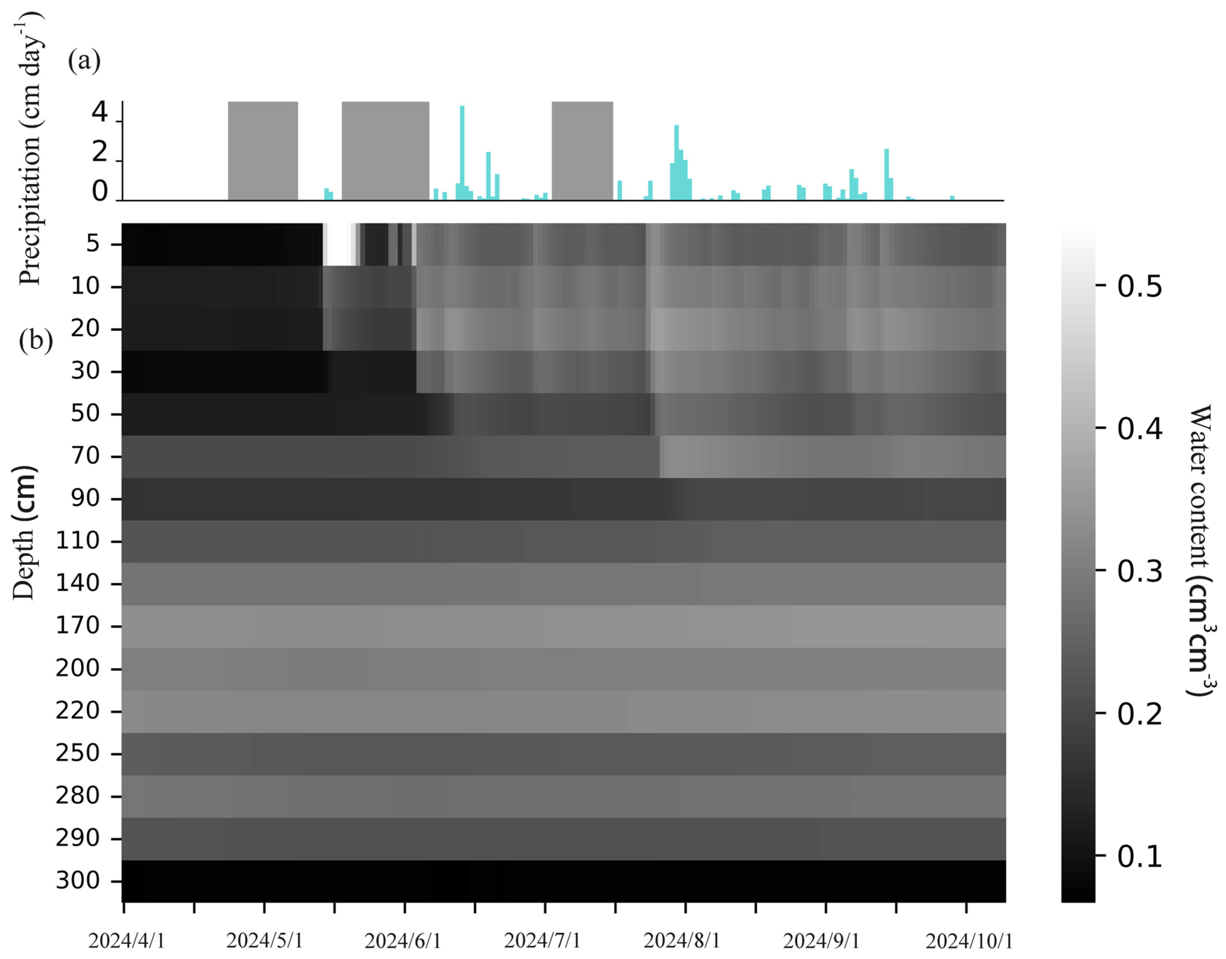
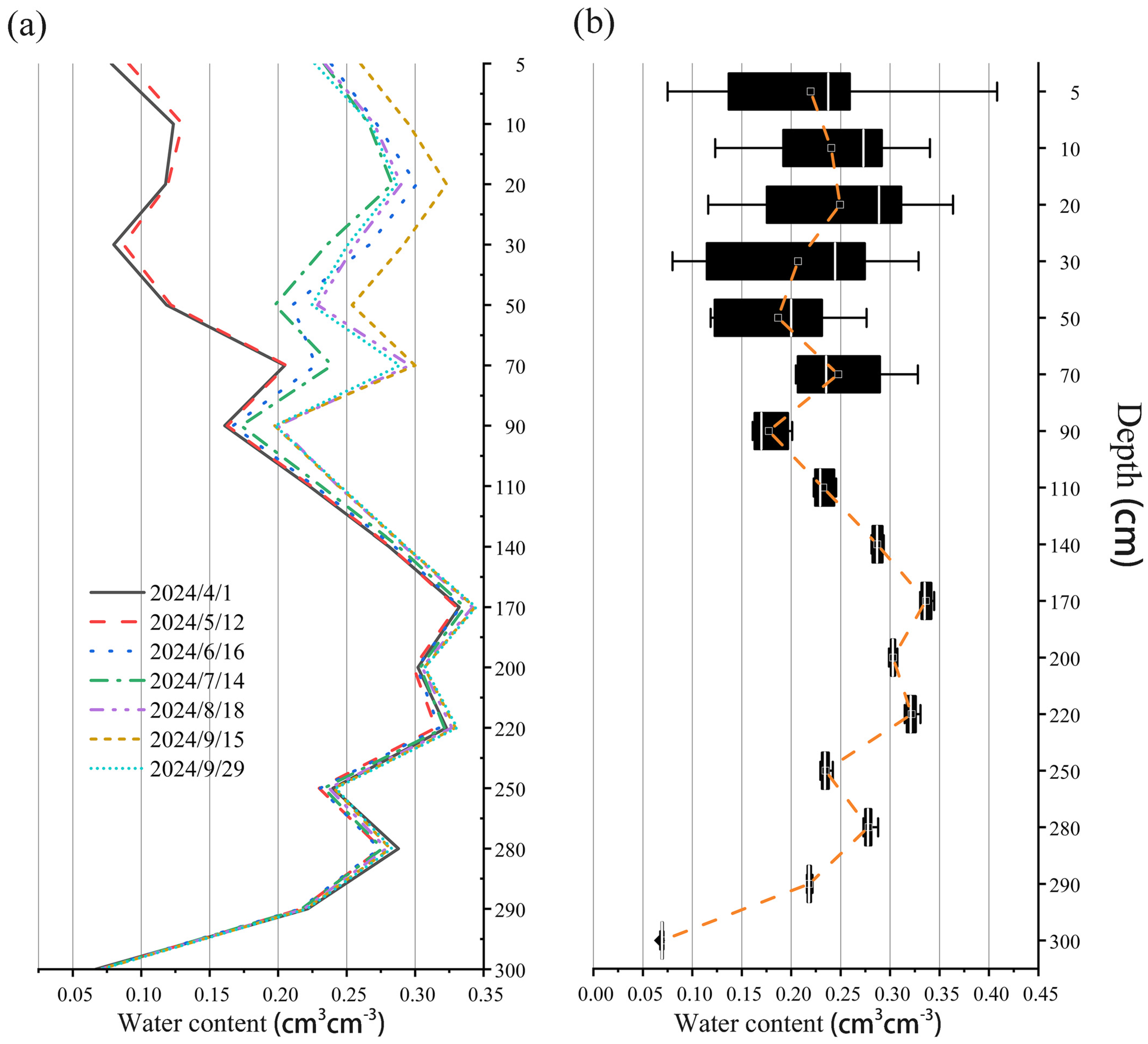
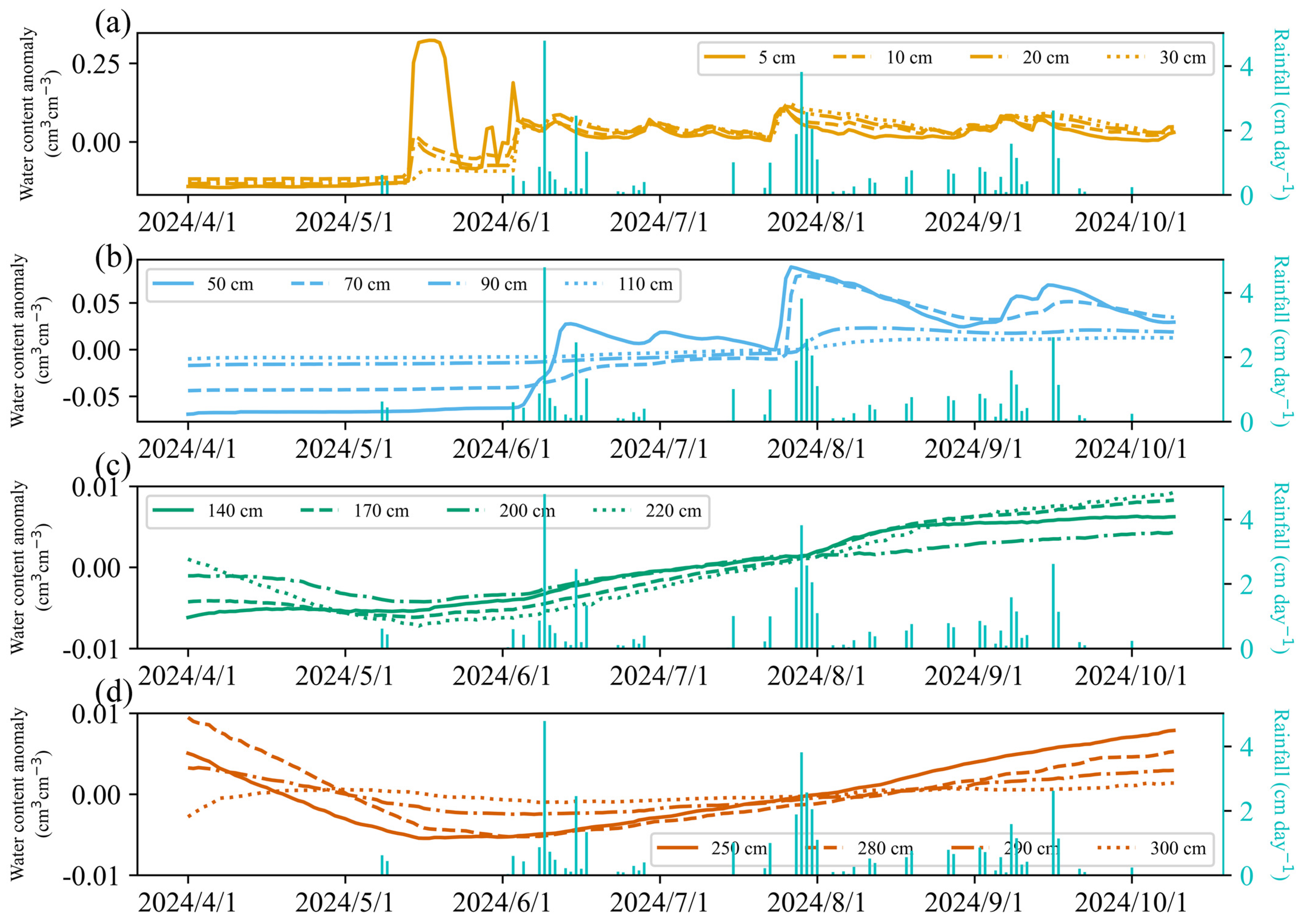
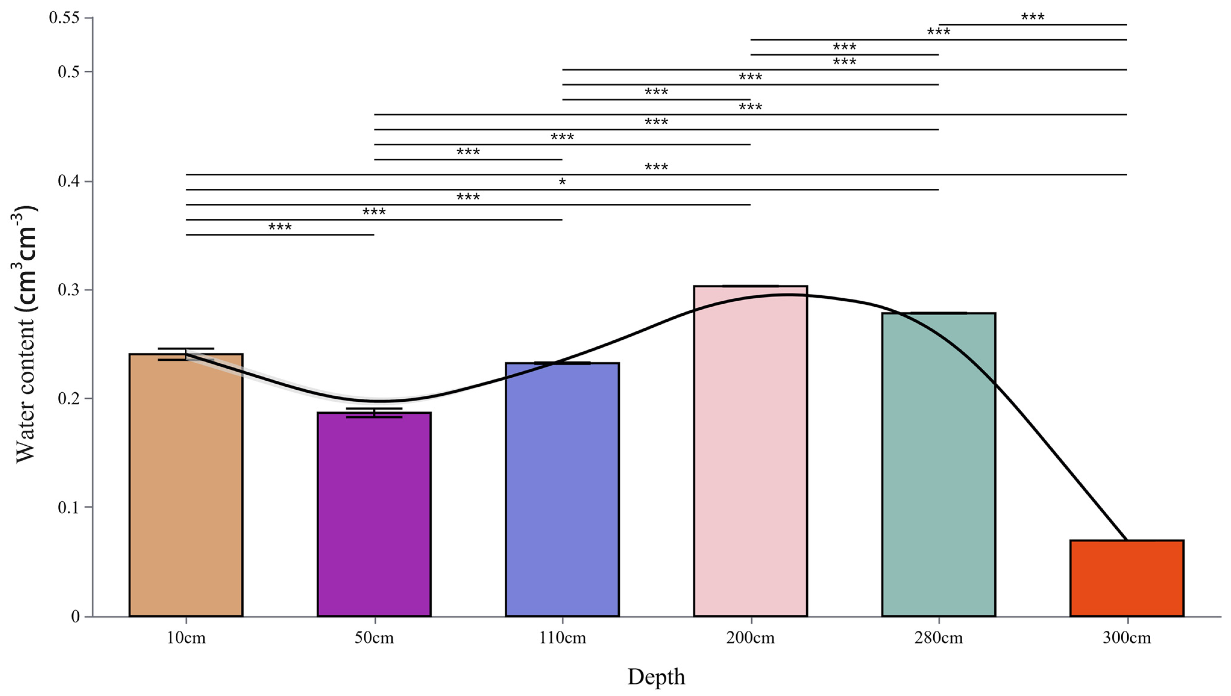
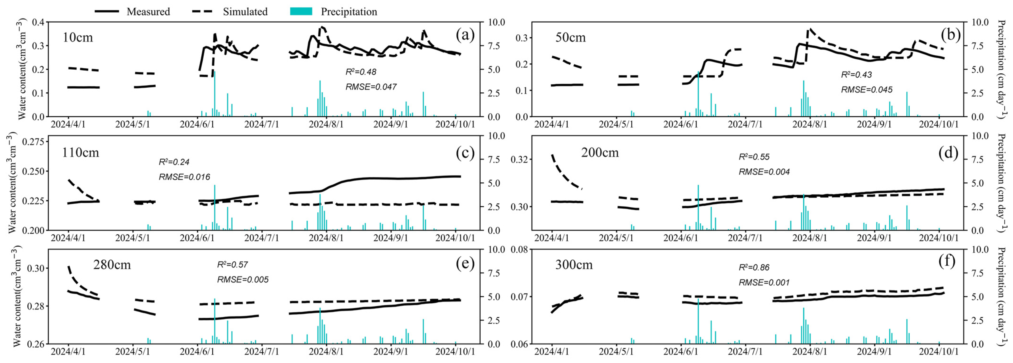
3.1. Soil Water Dynamics at Different Depths

Figure 3 shows the daily precipitation and soil water dynamics at different depths. Due to equipment maintenance issues, precipitation data for the three time periods of 16 April to 1 May, 12 May to 31 May, and 29 June to 12 July 2024 are missing (Figure 3a, shaded in gray), and the available precipitation data show concentrated heavy rainfall in mid-June and late July, with a gradual increase in rainfall from mid-August to mid-September. TDR monitoring showed that the soil water content in the deep layer (more than 70 cm underground) did not change significantly in the 6-month time scale, while the soil moisture content in the shallow layer (0–70 cm underground) changed significantly. It is worth noting that from early April to mid-May 2024, the average soil moisture content of 0–30 cm was less than 0.2 $\mathrm{c}{\mathrm{m}}^3{\mathrm{c}\mathrm{m}}^{-3}$, and the change was small.

According to the soil moisture content profile (Figure 4), with the increase in depth, the soil water content increased first and then decreased, reaching a peak at 170 cm underground, with an average water content of 0.33 $\mathrm{c}{\mathrm{m}}^3{\mathrm{c}\mathrm{m}}^{-3}$. At 300 cm underground, the average water content was 0.07 $\mathrm{c}{\mathrm{m}}^3{\mathrm{c}\mathrm{m}}^{-3}$. In order to observe the dynamic changes in the soil moisture profile, we extracted the soil moisture content for one day per month (Figure 4a), and it can be seen that in June 2024, the soil moisture content at a depth of 0–70 cm increased significantly compared with May, but the difference in soil moisture content at 90–300 cm was not large. In general, the soil moisture content of Haikou Forest Farm at a depth of 0–300 cm can be roughly divided into three levels, and the soil moisture content at 0–70 cm fluctuates significantly due to precipitation. The infiltration accumulation of soil water content at 70–170 cm continued to increase with depth and reached a peak. The soil moisture content at 170–300 cm gradually decreased with depth, and rapidly decreased from 0.22 to 0.07 $\mathrm{c}{\mathrm{m}}^3{\mathrm{c}\mathrm{m}}^{-3}$ after exceeding 290 cm. The soil moisture content at this level did not fluctuate significantly on the time scale of 6 months.

To more clearly demonstrate the dynamic changes in soil moisture, we employed the Anomalies method (daily precipitation minus average daily precipitation) to present the changes in soil moisture content at different depths within a single framework. To enhance readability, the soil water dynamics at 16 depths were categorized into four groups. Figure 5 shows that the soil moisture at a depth of 5 cm experienced a significant increase followed by a decrease in mid-May, while the soil moisture dynamics at 10, 20, and 30 cm were relatively consistent. As depth increased, soil water at depths of 50 and 70 cm exhibited considerable differences from April to July, but the trend became consistent from August to October. The soil moisture content at depths of 90 and 110 cm remained largely unchanged over the six-month period, with only a slight increase in early August, when precipitation was most concentrated. Soil moisture content in the range of 140 to 220 cm showed a slight decreasing trend from April to May, followed by a gradual increase, indicating that the moisture content in this layer accumulated throughout the observation period. In contrast, the soil moisture content at depths of 250 to 290 cm displayed a clear trend of decreasing and then increasing, reaching its lowest point at the end of May, with similar moisture content in April and October, indicating that this soil layer did not accumulate additional moisture.

We selected soil moisture content at different depths for differential analysis. From Figure 6, it can be observed that the differences in water content among the different soil layers are statistically significant; the p value between 10 cm and 280 cm is less than 0.05, while the p values between other soil layers are all less than 0.001.

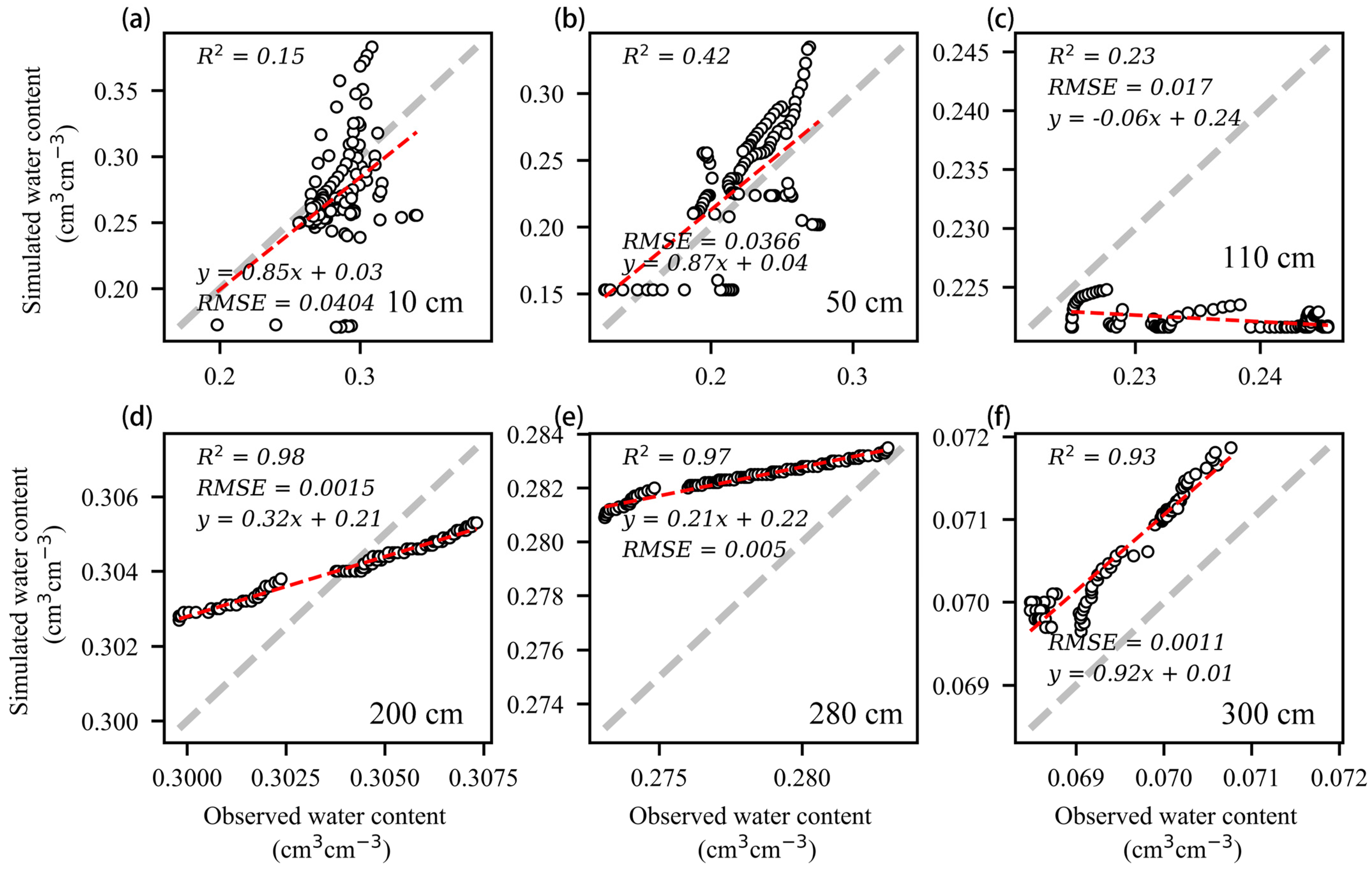
3.2. Model Simulation Results

Soil moisture content at different depths from April to October 2024 was modeled using Hydrus-1D, and Figure 7 shows the simulation and measurement results at depths of 10, 50, 110, 200, 280, and 300 cm. It can be seen that at depths of 10 and 50 cm, the ${\mathrm{R}}^2$ values between the model simulation results and the actual measurements are 0.48 and 0.43, respectively, and the model better reflects the events of increasing soil moisture content caused by rainfall, especially at the beginning of June and the end of July. However, although the model captures fluctuations in soil moisture content affected by precipitation, its response time is later than the actual situation, and at the beginning of the simulation (April–June), the model overestimates soil water content due to the lack of rainfall data. For the soil at a depth of 110 cm, the performance of the model decreased significantly, with an ${\mathrm{R}}^2$ of only 0.24. In addition, the model failed to accurately capture the soil moisture increase event in August and underestimated the soil moisture content between August and October. The model performed poorly for soil moisture dynamics at a depth of 200 cm, but between June and October, the simulated soil moisture content was close to the measured value, with an overall RMSE of 0.004 $\mathrm{c}{\mathrm{m}}^3 {\mathrm{c}\mathrm{m}}^{-3}$. In the deeper soil layers (280–300 cm), the performance of the model was improved, reaching ${\mathrm{R}}^2$ values of 0.57 and 0.86 from the measured values, respectively. The dynamics of the moisture content of these deep soils were not obvious, and the simulation results were similar in magnitude to the measured values, with RMSE values of 0.005 and 0.001 $\mathrm{c}{\mathrm{m}}^3 {\mathrm{c}\mathrm{m}}^{-3}$, respectively. In general, it is difficult for the model to accurately capture the soil moisture dynamics at the early stage of simulation, and it tends to overestimate the soil water content. However, between June and October, the model was able to better reflect soil moisture dynamics at depths of 10 and 50 cm, but its predictions were worse at depths of 110 and 200 cm. For deeper soil layers (280 and 300 cm), the model’s ability to simulate soil moisture dynamics improved.

Due to the lack of boundary conditions from early April to mid-July, we analyzed the simulation results from mid-July to October separately (Figure 8), and the results showed that the Hydrus-1D model seriously underestimated the actual soil moisture content at a depth of 110 cm and failed to capture the dynamic changes in soil moisture when the boundary conditions were intact. However, at deep layers (200–280 cm), the model shows a higher ${\mathrm{R}}^2$ value, but deviates significantly from the 1:1 line.

4. Discussion

This study enhances the current knowledge of soil moisture distribution in plantation forests and provides empirical validation for the Hydrus-1D model in deep soil conditions. In this section, we will discuss the results in terms of soil moisture content characteristics and possible driving factors, and evaluate the ability of Hydrus-1D simulation under the existing assumptions.

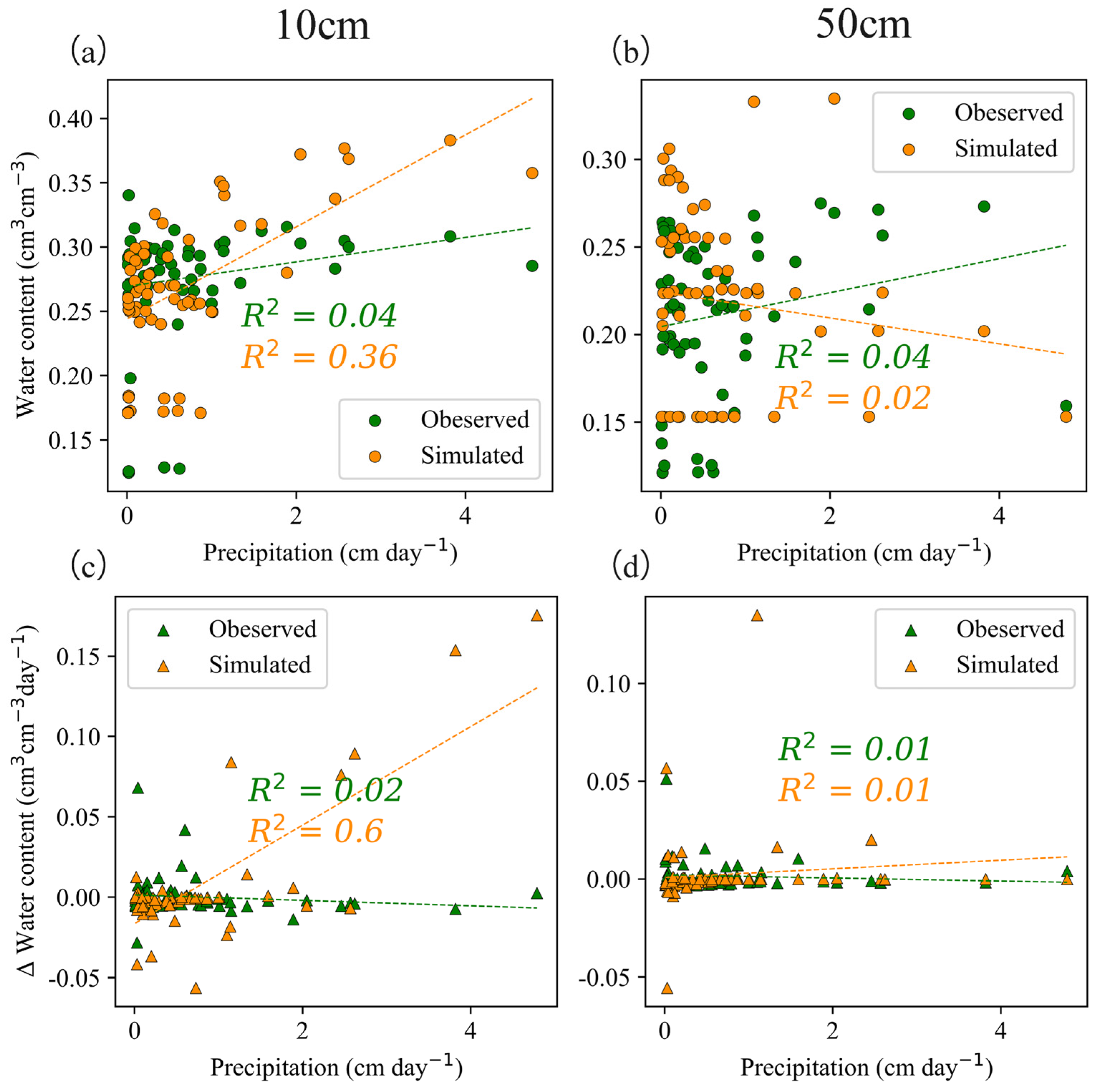
4.1. Vertical Variation Characteristics and Driving Forces of Soil Water Content

The vertical distribution characteristics of soil water content can be divided into three levels: the 0–70 cm layer, which fluctuates significantly under the influence of precipitation; the 70–170 cm layer, which gradually accumulates to a peak with increasing depth; and the 170–300 cm layer, which gradually decreases with increasing depth. This characteristic is closely related to the heterogeneity of soil hydraulic properties. In the active layer (0–70 cm), the soil may be mainly composed of sandy loam, with highly saturated water conductivity that allows the rapid infiltration of precipitation, but due to its weak water-holding capacity and the effect of surface evaporation, water loss is more obvious [39]. In the transitional accumulation layer (70–170 cm), the soil composition changes, resulting in a significant decrease in saturated water conductivity, and the retention time of water in this layer is prolonged, forming a natural “water retention zone”. The soil texture of the deep dissipative layer (170–300 cm) changed again, and although the water conductivity recovered, it was lower than that of the surface layer, so the water was mainly driven by gravity to infiltrate it, resulting in a decrease in water content with depth. In particular, a sharp decrease in water content was observed at a depth of 290 cm, which was associated with the groundwater boundary effect.

The water dynamics of the active layer (0–70 cm) are the result of the combined action of root water uptake and precipitation recharge. Pinus yunnanensis and Pinus huashanensis, the main tree species in the region, have root systems up to 90 cm deep, with 80% of their fine roots concentrated at a depth of 0–30 cm [40], resulting in the rapid depletion of water in this layer during the dry season. In deep soils of more than 60 cm, the water variation is smaller due to the lower root density, which is mainly driven by a slow substrate potential gradient [41]. In the early stage after precipitation, the root water uptake was temporarily inhibited, and the plant transpiration rate increased with the increase in soil water potential, but then with the recovery of soil water potential, the root water uptake rate returned to normal until the next precipitation event or reached a wilting point.

In addition, the recharge efficiency of soil moisture in the 0–70 cm layer is affected by rainfall and initial water content. Figure 9 shows that precipitation of low intensity (less than 0.5 ${\mathrm{c}\mathrm{m} \mathrm{h}\mathrm{o}\mathrm{u}\mathrm{r}}^{-1}$) was predominantly concentrated between April and October 2024. During these precipitation events, soil moisture content at a depth of 50 cm is usually lower than that at a depth of 10 cm, indicating that water slowly infiltrates downward in a stepped manner. By analyzing (Figure 9) the change in soil water content 1 h after a rainfall event ($∆\mathrm{W}\mathrm{a}\mathrm{t}\mathrm{e}\mathrm{r} \mathrm{c}\mathrm{o}\mathrm{n}\mathrm{t}\mathrm{e}\mathrm{n}\mathrm{t}$), it was found that the change in soil moisture at a depth of 10 cm was more significant within an hour than at a depth of 50 cm. Although the $∆\mathrm{W}\mathrm{a}\mathrm{t}\mathrm{e}\mathrm{r} \mathrm{c}\mathrm{o}\mathrm{n}\mathrm{t}\mathrm{e}\mathrm{n}\mathrm{t}$ at a depth of 10 cm was positively correlated with rainfall intensity, ${\mathrm{R}}^2=0.15$ indicates that rainfall intensity only explained 15% of the change, and other factors such as precipitation duration, rain pattern, soil initial conditions, and spatial heterogeneity were equally important. According to Darcy’s law, the lag in the response of deep soil moisture is limited by the average soil hydraulic conductivity, and a certain amount of precipitation accumulation is required to penetrate deeper into the soil.

4.2. Soil Water Simulations Require More Detailed Consideration

Hydrus-1D, based on the Richards equation and the van Genuchten–Mualem model, can simulate water transport in heterogeneous soils by inputting soil hydraulic parameters (such as saturated hydraulic conductivity, porosity, shape parameters, etc.) in layers. In the deep simulation (280–300 cm), the model showed high agreement with the measured values (${\mathrm{R}}^2$ = 0.57 to 0.86, RMSE = 0.001 to 0.005 $\mathrm{c}{\mathrm{m}}^3 {\mathrm{c}\mathrm{m}}^{-3}$), indicating that when the soil hydraulic parameters and boundary conditions are set accurately, Hydrus-1D can effectively simulate the slow migration process of low dynamic water. At depths of 10 cm and 50 cm, the model successfully captured precipitation-driven peaks in soil moisture content in early June and late July (${\mathrm{R}}^2$ = 0.43 to 0.48), which validates the model’s basic assumptions regarding the surface flux boundary and the root water uptake module (Feddes model). However, during periods of concentrated precipitation, the model indicated that the increase in soil moisture content at a depth of 10 cm lagged behind the actual measurements by about 2 to 3 days. This means that even a small amount of rainfall can impact soil moisture content after a period of drought, and the Hydrus-1D model is not sensitive enough to this rainfall infiltration process. The analysis shows (Figure 10) that when precipitation exceeds 1.5 $\mathrm{c}\mathrm{m} \mathrm{d}\mathrm{a}{\mathrm{y}}^{-1}$, the model tends to overestimate the response of shallow soil moisture, resulting in simulated soil moisture content that is higher than the actual value. In contrast, in deeper soil layers (e.g., 50 cm), the model is closer to the actual measurements (Figure 10d), which may imply a significant variation in water conductivity in the depth range of 0 to 50 cm, i.e., a significant heterogeneity between the soil layer at a depth of 10 cm and the underlying layer. However, the model still uses average hydraulic parameters for simulation, which does not fully reflect this heterogeneity. Therefore, in order to improve the accuracy of the model, it is necessary to more accurately determine the soil hydraulic parameters at different depths and consider the vertical change in soil texture to better capture the dynamic change characteristics of soil moisture. The abrupt change in hydraulic conductivity may also result in soil moisture movement dominated by preferential flow resulting from macropores such as wormholes and root pores. To address this issue, Hydrus-1D can be locally modified based on the actual measured soil texture parameters.

In addition, the Hydrus-1D model exhibits a high degree of sensitivity to the initial parameters. From the simulation results of the six different depths presented, it can be seen that at the beginning of the simulation, there was a large deviation between the model and the actual measured values, and even the dynamic changes in soil moisture were incorrectly simulated. This shows that the error of the initial conditional parameters can have a significant impact on the results at the beginning of the simulation. For example, if the model sets the initial water content to the field water holding capacity, when in fact the initial water content has decreased due to the influence of the dry season, the soil moisture content in the early stages of the simulation will be overestimated. The lack of meteorological data further exacerbates the problem, especially between April and June, and may lead to incorrect estimates of soil water recharge and surface evaporation in models. However, during the simulation period from June to October, the model is close to the measured values, indicating that it has strong mathematical stability in the simulation of continuous hydrological processes, especially for the prediction of seasonal water dynamics. Although the ${\mathrm{R}}^2$ value between the model and the measured values is high (0.57 to 0.86) in the depth range of 280–300 cm, the potential structural errors of the model may be masked due to the relatively weak soil moisture dynamics at these levels. For example, if the actual depth of groundwater differs from the model assumptions, the recharge of the 290–300 cm layer by capillary rising water will be ignored, resulting in cumulative errors in long-term simulations. It is worth noting that the underground terrain in the study area is mainly mountainous, and the underground runoff generated after the precipitation event will form a water-retaining zone in the underground soil layer, which is a complex hydrological process that is difficult to accurately simulate in the one-dimensional Hydrus model.

In this study, we lack detailed measurements of soil hydraulic parameters. According to the Richards equation, the void structure and water characteristic curves of different soils have a significant impact on the results. We utilize the parameter inversion method to obtain the main parameters in Hydrus-1D. Although this method can provide a preliminary assessment of the model’s simulation performance for soil water in plantations, it also limits our ability to reflect the actual conditions through the model. We believe that the main reason for the unsatisfactory simulation results in the depth range of 110 to 200 cm is the spatial heterogeneity of soil hydraulic parameters. The soil layer may have multiple abrupt changes in water conductivity, but in the model, the soil layer is only divided into three layers, each still using homogeneous parameterization, which can lead to an incorrect estimation of the water infiltration rate, resulting in a significant discrepancy between the simulated results and actual observations. Therefore, we should enhance the future simulation of soil water in plantations from two aspects: on one hand, through laboratory measurements and field inversions, multi-layer undisturbed soil column sampling experiments should be conducted on 300 cm soil to obtain accurate soil properties, soil water potential, and water characteristic curves; on the other hand, we can consider supplementing the coupled surface–subsurface model of Hydrus-1D or using more complex models like Hydrus-3D. Additionally, we can consider replacing the root water uptake module from the Feddes model with a dynamic root model to allow deep roots to reverse water transport through hydraulic redistribution during drought periods, combined with data on the seasonal growth of fine roots. At the same time, hydrometeorological models can be coupled with groundwater models (e.g., MODFLOW) [42,43] to achieve joint simulations of the ‘surface–groundwater’ continuum, thereby testing whether drops in deep water content are influenced by fluctuations in groundwater levels.

5. Conclusions

Previous studies have not monitored soil moisture at such depths with multiple segments and continuously. Our study reveals the detailed changes in soil moisture in plantations and whether conventional models can effectively simulate the dynamic processes of soil moisture. The observations indicate that there are significant differences in the vertical distribution of soil moisture, which can be classified into the active layer (0–70 cm), transitional accumulation layer (70–170 cm), and deep dissipation layer (170–300 cm). There are significant differences in the performance of the Hydrus-1D model at different time scales. From April to June, simulation errors accumulated due to the deviation in the initial condition setting and the lack of meteorological data. Between June and October, shallow simulations improved. The simulation results showed that there was a significant difference in the ability of Hydrus-1D to simulate soil moisture at 10–50 cm and 110–200 cm. In the shallow layer, the model successfully captured the precipitation-driven peak water content in early June and late July (${\mathrm{R}}^2=0.58$), but there was a lag period of 2–3 days in response to precipitation, and the lack of precipitation data in the early simulation (April–June) led to a systematic overestimation of water content. The 110–200 cm simulation capacity decreases ${(\mathrm{R}}^2=0.39)$ and fails to reflect the increase in water content triggered by heavy precipitation in August. The modelled deep soil water (280–300 cm) shows high accuracy due to weak water content dynamics, and is mainly affected by groundwater boundary conditions.

High-resolution and deep TDR monitoring addresses the previous inadequacies in soil water dynamics and provides evaluations for deep soil water models. Future efforts should focus on improving boundary conditions and long-term monitoring, including enhancing the spatial distribution of monitoring equipment, considering topographical factors and the lateral movement of soil moisture to enable deeper research into precipitation distribution and soil hydraulic dynamics in plantations.

References

1. Lyu, S.; Wang, J. Soil Water Stable Isotopes Reveal Surface Soil Evaporation Loss Dynamics in a Subtropical Forest Plantation. Forests 2021, 12, 1648. [Google Scholar] [CrossRef]
2. Evaristo, J.; Kim, M.; van Haren, J.; Pangle, L.A.; Harman, C.J.; Troch, P.A.; McDonnell, J.J. Characterizing the Fluxes and Age Distribution of Soil Water, Plant Water, and Deep Percolation in a Model Tropical Ecosystem. Water Resour. Res. 2019, 55, 3307–3327. [Google Scholar] [CrossRef]
3. Broedel, E.; Tomasella, J.; Cândido, L.A.; von Randow, C. Deep Soil Water Dynamics in an Undisturbed Primary Forest in Central Amazonia: Differences between Normal Years and the 2005 Drought. Hydrol. Process. 2017, 31, 1749–1759. [Google Scholar] [CrossRef]
4. Yang, F.; Feng, Z.; Wang, H.; Dai, X.; Fu, X. Deep Soil Water Extraction Helps to Drought Avoidance but Shallow Soil Water Uptake during Dry Season Controls the Inter-Annual Variation in Tree Growth in Four Subtropical Plantations. Agric. For. Meteorol. 2017, 234, 106–114. [Google Scholar] [CrossRef]
5. Zunzunegui, M.; Boutaleb, S.; Díaz Barradas, M.C.; Esquivias, M.P.; Valera, J.; Jáuregui, J.; Tagma, T.; Ain-Lhout, F. Reliance on Deep Soil Water in the Tree Species Argania Spinosa. Tree Physiol. 2017, 38, 678–689. [Google Scholar] [CrossRef] [PubMed]
6. Klein, T.; Rotenberg, E.; Cohen-Hilaleh, E.; Raz-Yaseef, N.; Tatarinov, F.; Preisler, Y.; Ogée, J.; Cohen, S.; Yakir, D. Quantifying Transpirable Soil Water and Its Relations to Tree Water Use Dynamics in a Water-Limited Pine Forest. Ecohydrology 2014, 7, 409–419. [Google Scholar] [CrossRef]
7. Spanner, G.C.; Gimenez, B.O.; Wright, C.L.; Menezes, V.S.; Newman, B.D.; Collins, A.D.; Jardine, K.J.; Negrón-Juárez, R.I.; Lima, A.J.N.; Rodrigues, J.R.; et al. Dry Season Transpiration and Soil Water Dynamics in the Central Amazon. Front. Plant Sci. 2022, 13. [Google Scholar] [CrossRef]
8. Stahl, C.; Hérault, B.; Rossi, V.; Burban, B.; Bréchet, C.; Bonal, D. Depth of Soil Water Uptake by Tropical Rainforest Trees during Dry Periods: Does Tree Dimension Matter? Oecologia 2013, 173, 1191–1201. [Google Scholar] [CrossRef]
9. Hasselquist, N.J.; Benegas, L.; Roupsard, O.; Malmer, A.; Ilstedt, U. Canopy Cover Effects on Local Soil Water Dynamics in a Tropical Agroforestry System: Evaporation Drives Soil Water Isotopic Enrichment. Hydrol. Process. 2018, 32, 994–1004. [Google Scholar] [CrossRef]
10. Acharya, B.S.; Dodla, S.; Wang, J.J.; Pavuluri, K.; Darapuneni, M.; Dattamudi, S.; Maharjan, B.; Kharel, G. Biochar Impacts on Soil Water Dynamics: Knowns, Unknowns, and Research Directions. Biochar 2024, 6, 34. [Google Scholar] [CrossRef]
11. Jiang, Z.-Y.; Wang, X.-D.; Zhang, S.-Y.; He, B.; Zhao, X.-L.; Kong, F.-L.; Feng, D.; Zeng, Y.-C. Response of Soil Water Dynamics to Rainfall on A Collapsing Gully Slope: Based on Continuous Multi-Depth Measurements. Water 2020, 12, 2272. [Google Scholar] [CrossRef]
12. Njana, M.A.; Mbilinyi, B.; Eliakimu, Z. The Role of Forests in the Mitigation of Global Climate Change: Emprical Evidence from Tanzania. Environ. Chall. 2021, 4, 100170. [Google Scholar] [CrossRef]
13. Wang, Y.; He, Y.; Li, Z.; Qu, J.; Wang, G. Soil Water Dynamics and Deep Percolation in an Agricultural Experimental Area of the North China Plain over the Past 50 Years: Based on Field Monitoring and Numerical Modeling. Sci. Total Environ. 2024, 928, 172367. [Google Scholar] [CrossRef] [PubMed]
14. Srivastava, P.K. Satellite Soil Moisture: Review of Theory and Applications in Water Resources. Water Resour. Manag. 2017, 31, 3161–3176. [Google Scholar] [CrossRef]
15. Chen, T.; McVicar, T.R.; Wang, G.; Chen, X.; De Jeu, R.A.M.; Liu, Y.Y.; Shen, H.; Zhang, F.; Dolman, A.J. Advantages of Using Microwave Satellite Soil Moisture over Gridded Precipitation Products and Land Surface Model Output in Assessing Regional Vegetation Water Availability and Growth Dynamics for a Lateral Inflow Receiving Landscape. Remote Sens. 2016, 8, 428. [Google Scholar] [CrossRef]
16. Saxton, K.E.; Rawls, W.J. Soil Water Characteristic Estimates by Texture and Organic Matter for Hydrologic Solutions. Soil Sci. Soc. Am. J. 2006, 70, 1569–1578. [Google Scholar] [CrossRef]
17. An, N.; Tang, C.-S.; Cheng, Q.; Wang, D.-Y.; Shi, B. Laboratory Characterization of Sandy Soil Water Content during Drying Process Using Electrical Resistivity/Resistance Method (ERM). Bull. Eng. Geol. Environ. 2020, 79, 4411–4427. [Google Scholar] [CrossRef]
18. Jeřábek, J.; Zumr, D.; Dostál, T. Identifying the Plough Pan Position on Cultivated Soils by Measurements of Electrical Resistivity and Penetration Resistance. Soil Tillage Res. 2017, 174, 231–240. [Google Scholar] [CrossRef]
19. Tamboli, P.M. The Influence of Bulk Density and Aggregate Size on Soil Moisture Retention. Ph.D. Thesis, Iowa State University of Science and Technology, Iowa, IA, USA, 1961. [Google Scholar]
20. Balaghi, S.; Ghal–Eh, N.; Mohammadi, A.; Vega–Carrillo, H.R. A Neutron Scattering Soil Moisture Measurement System with a Linear Response. Appl. Radiat. Isot. 2018, 142, 167–172. [Google Scholar] [CrossRef]
21. Gardner, W.R.; Kirkham, D.J. Determination of Soil Moisture by Neutron Scattering. Soil Sci. 1952, 73, 391–402. [Google Scholar] [CrossRef]
22. Zawilski, B.M.; Granouillac, F.; Claverie, N.; Lemaire, B.; Brut, A.; Tallec, T. Calculation of Soil Water Content Using Dielectric-Permittivity-Based Sensors—Benefits of Soil-Specific Calibration. Geosci. Instrum. Methods Data Syst. 2023, 12, 45–56. [Google Scholar] [CrossRef]
23. Robinson, D.A.; Campbell, C.S.; Hopmans, J.W.; Hornbuckle, B.K.; Jones, S.B.; Knight, R.; Ogden, F.; Selker, J.; Wendroth, O. Soil Moisture Measurement for Ecological and Hydrological Watershed-Scale Observatories: A Review. Vadose Zone J. 2008, 7, 358–389. [Google Scholar] [CrossRef]
24. Fan, J.; Scheuermann, A.; Guyot, A.; Baumgartl, T.; Lockington, D.A. Quantifying Spatiotemporal Dynamics of Root-Zone Soil Water in a Mixed Forest on Subtropical Coastal Sand Dune Using Surface ERT and Spatial TDR. J. Hydrol. 2015, 523, 475–488. [Google Scholar] [CrossRef]
25. Sposito, G. The Statistical Mechanical Theory of Water Transport through Unsaturated Soil: 2. Derivation of the Buckingham-Darcy Flux Law. Water Resour. Res. 1978, 14, 479–484. [Google Scholar] [CrossRef]
26. Sławiński, C.; Sobczuk, H. Soil–Plant–Atmosphere Continuum. In Encyclopedia of Agrophysics; Gliński, J., Horabik, J., Lipiec, J., Eds.; Springer: Dordrecht, The Nederlands, 2011; pp. 805–810. [Google Scholar] [CrossRef]
27. Werner, C.; Dubbert, M. Resolving Rapid Dynamics of Soil–Plant–Atmosphere Interactions. New Phytol. 2016, 210, 767–769. [Google Scholar] [CrossRef]
28. Orlowski, N.; Rinderer, M.; Dubbert, M.; Ceperley, N.; Hrachowitz, M.; Gessler, A.; Rothfuss, Y.; Sprenger, M.; Heidbüchel, I.; Kübert, A.; et al. Challenges in Studying Water Fluxes within the Soil-Plant-Atmosphere Continuum: A Tracer-Based Perspective on Pathways to Progress. Sci. Total Environ. 2023, 881, 163510. [Google Scholar] [CrossRef]
29. Chali, A.K.N.; Hashemi, S.R.; Akbarpour, A. Numerical Solution of the Richards Equation in Unsaturated Soil Using the Meshless Petrov–Galerkin Method. Appl. Water Sci. 2023, 13, 119. [Google Scholar] [CrossRef]
30. Vereecken, H.; Schnepf, A.; Hopmans, J.W.; Javaux, M.; Or, D.; Roose, T.; Vanderborght, J.; Young, M.H.; Amelung, W.; Aitkenhead, M.; et al. Modeling Soil Processes: Review, Key Challenges, and New Perspectives. Vadose Zone J. 2016, 15, vzj2015-09. [Google Scholar] [CrossRef]
31. Sadeghi, M.; Hatch, T.; Huang, G.; Bandara, U.; Ghorbani, A.; Dogrul, E.C. Estimating Soil Water Flux from Single-Depth Soil Moisture Data. J. Hydrol. 2022, 610, 127999. [Google Scholar] [CrossRef]
32. Rai, V.; Pramanik, P.; Das, T.K.; Aggarwal, P.; Bhattacharyya, R.; Krishnan, P.; Sehgal, V.K. Modelling Soil Hydrothermal Regimes in Pigeon Pea under Conservation Agriculture Using Hydrus-2D. Soil Tillage Res. 2019, 190, 92–108. [Google Scholar] [CrossRef]
33. Gabiri, G.; Burghof, S.; Diekkrüger, B.; Leemhuis, C.; Steinbach, S.; Näschen, K. Modeling Spatial Soil Water Dynamics in a Tropical Floodplain, East Africa. Water 2018, 10, 191. [Google Scholar] [CrossRef]
34. Mo’allim, A.A.; Kamal, M.R.; Muhammed, H.H.; Yahaya, N.K.E.M.; Zawawe, M.A.B.M.; Man, H.B.C.; Wayayok, A. An Assessment of the Vertical Movement of Water in a Flooded Paddy Rice Field Experiment Using Hydrus-1D. Water 2018, 10, 783. [Google Scholar] [CrossRef]
35. Allen, R.G.; Pereira, L.S.; Raes, D.; Smith, M. Crop Evapotranspiration: Guidelines for Computing Crop Water Requirements. Fao Rome 1998, 300, D05109. [Google Scholar]
36. Richards, L.A. Capillary Conduction of Liquids Through Porous Mediums. Physics 1931, 1, 318–333. [Google Scholar] [CrossRef]
37. Feddes, R.A.; Kowalik, P.J.; Zaradny, H. Simulation of Field Water Use and Crop Yield; John Wiley & Sons Inc.: Hoboken, NJ, USA, 1978. [Google Scholar]
38. Rabbel, I.; Bogena, H.; Neuwirth, B.; Diekkrüger, B. Using Sap Flow Data to Parameterize the Feddes Water Stress Model for Norway Spruce. Water 2018, 10, 279. [Google Scholar] [CrossRef]
39. Wang, Y.; Ma, R.; Zhu, G. Representation of the Influence of Soil Structure on Hydraulic Conductivity Prediction. J. Hydrol. 2023, 619, 129330. [Google Scholar] [CrossRef]
40. Altinalmazis-Kondylis, A.; Muessig, K.; Meredieu, C.; Jactel, H.; Augusto, L.; Fanin, N.; Bakker, M.R. Effect of Tree Mixtures and Water Availability on Belowground Complementarity of Fine Roots of Birch and Pine Planted on Sandy Podzol. Plant Soil 2020, 457, 437–455. [Google Scholar] [CrossRef]
41. Knipfer, T. Future in the Past: Water Uptake Function of Root Systems. Plant Soil 2022, 481, 495–500. [Google Scholar] [CrossRef]
42. Kim, N.W.; Chung, I.M.; Won, Y.S.; Arnold, J.G. Development and Application of the Integrated SWAT–MODFLOW Model. J. Hydrol. 2008, 356, 1–16. [Google Scholar] [CrossRef]
43. Sheikha-BagemGhaleh, S.; Babazadeh, H.; Rezaie, H.; Sarai-Tabrizi, M. The Effect of Climate Change on Surface and Groundwater Resources Using WEAP-MODFLOW Models. Appl. Water Sci. 2023, 13, 121. [Google Scholar] [CrossRef]
Figure 1. (a) Location map of the study site. (b) Satellite image of the study area. (c) Daily data of precipitation and PET during the study period, where black shading indicates the periods of missing data. (d) Photo of the TDR and automatic meteorological detection equipment.
Water 17 01199 g001
Figure 2. (a) The changes in measured and simulated soil moisture content at different depths during the calibration period, where solid lines represent the measured values, dashed lines represent the simulated values, and different colors indicate different depths. (b) Scatter plot of the measured and simulated values during the calibration period, with the red dashed line representing the linear fitting results.
Water 17 01199 g002
Figure 3. (a) Daily precipitation, with gray shaded areas indicating periods of missing data. (b) Chart of soil moisture content at different depths for each day, where close to white indicates high soil moisture content and close to black indicates lower soil moisture content.
Water 17 01199 g003
Figure 4. (a) Variation in soil moisture content with depth over time, with different colors representing different times. (b) Box plots of soil moisture content at different depths, where the white vertical lines indicate the median, the black squares indicate the mean, and the orange dashed line connects the mean soil moisture content at different depths.
Water 17 01199 g004
Figure 5. (ad) The changes in soil moisture content measured at different depths, with the histogram representing daily precipitation and each subplot displaying the changes in soil moisture content at four different depths.
Water 17 01199 g005
Figure 6. There are significant differences in soil water content between different depths. * indicates significant differences at p < 0.05; and *** at p < 0.001. The black curve represents the trend line.
Water 17 01199 g006
Figure 7. (af) Comparison of simulated and measured soil moisture content at different depths from 1 April 2024 to 3 October 2024, where the black solid lines represent the measured values, the dashed lines represent the simulated values, and the blue bar chart represents daily precipitation.
Water 17 01199 g007
Figure 8. (af) Scatter plots of measured and simulated soil moisture content at different depths from 15 July to 3 October 2024, with the red dashed lines representing the linear regression results and the gray dashed lines representing the 1:1 line.
Water 17 01199 g008
Figure 9. (a,b) The responses of soil moisture content at depths of 10 cm and 50 cm to hourly precipitation. (c,d) The responses of delta soil moisture content at depths of 10 cm and 50 cm to hourly precipitation. The green dashed lines represent the linear regression results.
Water 17 01199 g009
Figure 10. (a,b) The responses of soil moisture content at depths of 10 cm and 50 cm to daily precipitation. (c,d) The responses of W a t e r   c o n t e n t at the same depths to daily precipitation. The green markers represent the measured values, the orange markers represent the simulated values, and the dotted lines represent the linear regression results.
Water 17 01199 g010