Abstract
Water and wastewater monitoring plays a fundamental role in understanding the impact of anthropogenic activities on natural systems. Statistical process control (SPC) is a technique, among other statistical methods, for controlling systems and improving quality, with early applications in water quality and wastewater monitoring. This study aims to clarify the basic concepts of the tool, study how it has been used in water and wastewater monitoring, and highlight the limitations and opportunities for research. SPC still needs necessary adaptations and considerations to deal with the limitations of environmental data, especially in open systems such as water bodies. Future research should explore suitable statistical parameters and chart options, which could represent financial savings and effectiveness in monitoring, as, to date, the choice of these parameters has been based on monitoring studies conducted at the industrial level, where the variability in the monitoring variables is easily controlled. Finally, the tool shows promise for potential use in extreme events, such as droughts, major floods, storms (cyclones), and catastrophic environmental incidents (such as dam bursts), as long as the analysis is supported by a base period.
1. Introduction
The discharge of contaminants from raw or insufficiently treated wastewater, together with diffuse surface pollution, degrades water quality and thus compromises the various uses of water resources. This scenario is concerning since, due to urbanization, population growth, and the increase in industrial and agricultural activities, the global demand for water is on the rise. In certain parts of the world, the demand for water has exceeded its availability [1]. Results indicate that the degradation in water quality has contributed to an increase in the percentage of the global population suffering from water scarcity from 30% to 40% between 2000 and 2010 [2].
For multiple uses of water resources to be preserved, it is necessary to meet water quality standards, which are generally defined in national legislation according to classes and/or ranges based on their predominant uses. To meet these standards, it is necessary to monitor and control the use of surface water. Environmental monitoring plays a fundamental role in understanding the impact of anthropogenic activities on natural systems [3]. Environmental monitoring is conducted by monitoring the parameters used to indicate the quality of water for supply, wastewater, springs, and receiving bodies (von Sperling, 2014) [4]. Owing to temporal and spatial variations in the physical, chemical, and biological parameters of water quality, frequent monitoring programs are necessary. As a result, the large and complex databases generated contain a large amount of information related to the spatial and temporal patterns of surface water quality.
Statistical process control (SPC) is a technique, among other statistical methods, for controlling systems and improving quality [5] that can be used to understand spatiotemporal patterns in environmental monitoring. SPC is most commonly used in industrial processes; however, according to Montgomery [6], this tool can also be applied to non-industrial processes. SPC has already been applied to a variety of topics outside the industry, including sediment quality monitoring [7], the detection of blockages near sewage overflow sites [8], flood control [9], drought monitoring [10], and the study of indicator variables for the rupture of water distribution pipes [11]. Other studies have demonstrated the ability of SPC evaluation as a risk management tool that can indicate the occurrence of pollution episodes [12,13,14], as well as for controlling indicator variables for the performance of water and wastewater treatment plants [15,16].
Despite some published research initiatives, the potential of this tool is still poorly understood and explored by water resource management [17]. Thus, this study aims to clarify the basic concepts of the tool, as well as to study how it has been used in water and wastewater monitoring and to highlight the limitations and opportunities for research. To this end, this review has been organized into four sections: (i) an introduction to the subject and presentation of the problem, (ii) a presentation of the basic assumptions of SPC, (iii) a description of the application of SPC in recent work, with an indication of limitations and gaps, and (iv) the conclusions and recommendations of this work.
2. Basic Concepts of Statistical Process Quality Control
A classic definition of the term “process” refers to any set of conditions or causes that work together to produce a certain result [18]. In general, the quality of any product or process can be measured using statistical tools that produce solid and consistent results in terms of controlling the variability in the parameters of interest [19]. Statistical process quality control (SPC) is a statistical method used to control systems and improve quality [5]. SPC was developed in 1924 by Walter Andrew Shewhart at Bell Telephone Laboratories based on the development of control charts, one of the main SPC techniques [6].
In SPC, the quality of a product (or service) is related to the variability in its characteristics [20]. Thus, the aim of SPC is to carry out control, ensuring that the quality characteristics are maintained within pre-established limits. The primary function of SPC is to reduce variability [5].
However, every process has inherent natural variability regardless of how well it is designed and controlled. This natural or random variability (or background noise) is the result of the cumulative effect of various causes that are unavoidable in their essence. As random causes are inherent to the process, the process is considered to be under statistical control, and most of its output is between the so-called “specification limits” [6]. Furthermore, a process under statistical control produces predictable results in probabilistic terms [21].
In addition to random causes, the process can also be subject to assignable (or special) causes, which can be eliminated using corrective measures. These causes lead to much larger variations compared to background noise, producing an unacceptable level of performance. When the process operates in the presence of assignable causes, it is “out of control”, and the product or service often has characteristics outside specified limits [22].
Thus, Montgomery [6] states that the variability that needs to be reduced is unwanted variability, that is, attributable variability. To achieve reduction, the tool must effectively identify unwanted variability. This is performed by establishing control or specification limits. Once identified, the next step is to remove variability through corrective action.
2.1. Process Control Charts
SPC tools are divided into histograms, control sheets, Pareto charts, cause-and-effect diagrams, defect concentration diagrams, scatter diagrams, and control charts [6]. Because they have been used in the literature to monitor the quality of water and wastewaters, control charts were the focus of this study.
Control charts are composed of upper and lower limits, as well as central lines, in which a given characteristic of interest can be monitored. There are four types of control charts that are divided according to the characteristics being monitored:
- Control charts for averages: These are also known as the control charts. They monitored the variation in the average. They will be more focused on in this work because they are usually used in the environmental monitoring of water quality and wastewaters.
- Control charts for variance: Monitor the variability in the process variance.
- Control charts for proportion of faults (p-charts): Monitor the fraction of faulty items.
- The control charts for the number of defects (c-charts) graphically express the number of defective items.
There are three basic types of control charts for average and variance: Shewart charts, exponentially weighted moving average (EWMA) charts, and cumulative sum (CUSUM) charts. Figure 1 shows three examples of Shewart control charts for the averages. Shewart charts are the most commonly used charts for monitoring processes. The following explanation focuses on understanding the monitoring process using Shewart charts and is based on the explanations of von Sperling et al. [5] and Ribeiro Jr [21]. The EWMA and CUSUM charts cover separate topics.
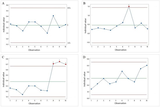
Figure 1.
Examples of Shewart’s control charts for averages. The points can represent any environmental parameter. Process under statistical control (A); attributable cause manifestation for a short period (B); process change (C); constant trend or shift in the data (D).
In Shewart’s charts for averages, each plotted point represents the average of the values sampled for a given parameter in a given unit of time, called subgroup m. The central line represents the average value of the quality characteristic, that is, the average of the subgroup averages. Two other horizontal lines, the upper control limit (UCL) and lower control limit (LCL) are also projected. In the case of individual sampling, which is common in environmental data, each plotted point represents a single sampled value (no division into subgroups).
According to Montgomery [6], the process control chart resembles a hypothesis test for the averages. It is assumed that the population and sample means for a normally distributed dataset are equal to and , and the sample and population standard deviations are given by σ and s. If the sample value lies between the limits set by the confidence interval, it can be said that the process mean is equivalent to and the process is under statistical control. However, if is outside this interval, the hypothesis is rejected, the process mean is equivalent to a value other than , called and the process is outside the state of statistical control.
Thus, if the process is under statistical control (i.e., the process mean is stable and variation is only due to unavoidable causes), a large percentage of the monitored points (determined by the confidence level) must be within the region defined by LCL and USL, and the sampling points must follow a random pattern, as shown in Figure 1A. Therefore, it is necessary to select a value of α that determines the confidence interval. When the data follows a normal distribution, or can be normalized using a statistical transformation technique, in order to be considered under control, 68.27% of future data must be within one standard deviation of the population mean, 95.45% of future data must be within 2σ of the mean, and 99.73% must be within 3σ of the mean. Thus, if the data follow a normal distribution, almost all points sampled should be located within the UCL and LCL, defined by three standard deviations from the mean, following an unsystematic oscillation [5].
However, when a sample is above or below the control limit, an attributable cause influences the performance of the process. In the example in Figure 1B, there are ten points, one of which is outside the control limits and represents 10% of the points outside the limits. Adopting a significance level of α = 1%, in which the null hypothesis is that the process is stable for the evaluated statistical parameter (in this case, the mean), the null hypothesis must be rejected. Therefore, the process was not statistically controlled.
According to Montgomery [6], changes due to attributable causes can manifest in different ways. The average can change to a new value and the oscillation pattern can remain around the new level. The attributable cause can manifest itself for a short period, causing an abrupt deviation from the average, but with its rapid return to the same level (Figure 1B), or the process can change, taking on different characteristics from the previous level (Figure 1C). In addition, there may have been a constant trend or shift in the data (Figure 1D).
Thus, by establishing the significance level, the control limits LCL and UCL are given by Equations (1) and (2), respectively, and the standard deviation of the sample mean is given by Equation (3).
where is the average of the entire dataset for a given parameter evaluated, is the number of standard deviations from the mean determined from α, is the standard deviation of the sample mean, and n is the number of observations per subgroup.
Owing to various limitations in the monitoring process, the sample size is sometimes n = 1, that is, the sample consists of a single observation, which is common in environmental water quality monitoring data. In such cases, it is necessary to apply control charts to the individual measurements. Each plotted point in this type of graph represents an observation.
2.2. Phases of Statistical Control
In practice, SPC using control charts comprises two phases. Phase 1 is a retrospective analysis phase, while in Phase 2, the aim is to carry out a prospective inspection of the process under investigation [12]. The construction of the control chart that will be used for monitoring in Phase 2 is carried out in Phase 1.
The main function of SPC is to identify the influence of the special causes acting on the process. Because this identification is based on establishing control limits from the variability of the sampled points, only points that are under the effect of natural or random causes can be located within the range established by the LCL and UCL. Thus, the main objective of Phase 1 is to test historical data to identify whether these data were collected in a period in which there were only random causes acting on the process [20].
Thus, in Phase 1, preliminary samples were used to construct preliminary (i.e., tentative) control limits. Montgomery [6] recommends at least 20–25 subgroups of n ranging from 3 to 5, or 20–25 samples in the case of individual measurements. According to the author, these number of samples should be sufficient to estimate average and standard deviation during an in control process period. Ribeiro Jr [21] mentioned that 25 subgroups are usually used, without specifying the recommended size n for subgroups.
In Phase 1, the first step is to plot the data on a control chart and analyze whether all points are within the tentative control limits and whether there is no systematic pattern. If these conditions are verified, the graph generated in this stage can be used in phase 2 to monitor the process [23].
However, if there are non-random patterns that indicate instability or even points outside the control limits, there are indications that assignable causes act on the process. Ideally, a special cause should be assigned to each out-of-control point. Then, the points outside the limit are not included in the determination of the control limits, and a review of the control limits is conducted. This process was repeated until all points were under control [6]. However, sometimes it is not possible to assign a particular cause to out-of-control points. Montgomery [6] recommends keeping only one or two points, as this will not result in significant distortions of the control limits.
According to Koutras et al. [20], once the control limits are established in Phase 1, the aim of Phase 2 is to monitor future data as to its state of statistical control. To do this, each observation is usually tested with the aid of a set of specific rules that help infer the existence of special causes. Shewart’s control charts have the disadvantage of ignoring information provided by entire sequences of points, as each plotted point only contains information from a single sample. This makes Shewart’s charts insensitive to small and medium process variations. To overcome this disadvantage, rules that increase the sensitivity of a graph can be used. These sensitizing rules make it possible to identify systematic patterns of imbalance in the sequence of points, which indicates a certain instability even if the samples assume values within the control limits [6].
The Shewart chart can be divided into three zones: Zone C contains points that are within 1 σ of the center line, Zone B contains points that are between 1 and 2 σ of the center line, and Zone A contains points between 2 and 3 σ of the center line. The rules in Table 1, known as Shewart’s rules, can be used to suggest out-of-control processes. Figure 2 shows their representation in Shewart’s graph.

Table 1.
Shewart’s rules. Source: Adapted from Boffoli et al. [24].
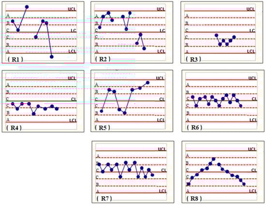
Figure 2.
Representation of Shewart’s rules. Details on each rule are provided on Figure 1. Source: Adapted from Boffoni et al. [24].
In addition to the rules described above, according to Koutras et al. [20], many sensitivity rules have been proposed by other authors. However, the same authors pointed out that the use of sensitizing rules can increase the incidence of false alarms. For this reason, the authors discourage the use of Shewart’s charts with sensitizing rules for Phase 2 and encourage the use of more efficient EWMA and CUSUM charts.
2.3. Exponentially Weighted Moving Average Charts and Cumulative Sums
It is known that Shewart charts are not very sensitive to small changes. Thus, exponentially weighted moving average (EWMA) and cumulative sum (CUSUM) graphs are recommended for detecting small and medium shifts on average, as each plotted point carries information on a long sequence of samples [20].
The CUSUM charts were proposed by Page [25]. Unlike EWMA, which gives greater weight to the most recent observations, CUSUM charts give equal weight to all observations [26]. In this type of SPC chart, each plotted value corresponds to the cumulative sum of the deviations of the sample values from a target value (often the average of all sampled data).
Roberts [27] introduced the EWMA chart. In the EWMA chart, the decision regarding the state of the process is based on information from each point plotted with a weight percentage from previous samples [21]. Equations (4)–(7) define the EWMA chart for individual observations.
where i ranges from 0 to m, m is the total number of subgroups (or number of points plotted on the graph), zi is the value plotted on the EWMA graph, λ is the smoothing parameter, xi is the value of the individual observation in the case of the EWMA graph for individual measurements (when n = 1), µ0 is the mean of the entire dataset, and L is the number of standard deviations σ from the mean µ0 used, that is, the width of the control limits.
The EWMA chart allows for the accumulation of information based on successive weightings so that more recent observations are weighted more heavily than older ones [26]. Parameter λ, which varies from 0 to 1, determines the weighting criterion. The closer it is to 1, the less sensitive the graph is to detect small changes, and, therefore, the less influence older samples have. According to Montgomery [6], 0.05 ≤ λ ≤ 0.25 is generally used, with values of 0.05, 0.10, and 0.20 being recurrent choices. Figure 3A and Figure 3B show examples of EWMA and CUSUM graphs, respectively.
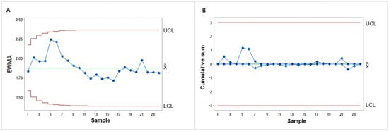
Figure 3.
Examples of EWMA (A) and CUSUM (B) graphs.
2.4. Process Capability Indices
The monitoring of any product or process must include an assessment of whether it meets the specifications. Capacity analysis compares the inherent variability of the process with the recommended or mandatory limits [28]. According to Ribeiro Jr [21], for capacity analysis, the stability of the process must first be verified, and this step can be performed using control charts. If the process is stable, that is, there are no special causes at work, a process capability analysis is carried out. Even if it is stable (under control), a process can be incapable of generating results that are not in line with what is required. In this case, corrective actions must be taken to bring the average and variability in the process to acceptable levels.
Capability analysis can be performed using a process capability index or ratio. The capability ratio of a process is a measure of its ability to produce results that meet specifications [6]. According to Corbett and Pan [28], this is an important risk management tool for professionals, as it allows them to infer the risk of the process causing noncompliance problems, as well as for regulators, as it contains useful information for inspection.
The process capability index is a numerical value that expresses the ratio between the variability in a process and its specification limit [29]. It is worth emphasizing that specification limits have no mathematical or statistical relationship with control limits [5]. While control limits are defined based on the natural variability of the process, specification limits are determined externally to the process, sometimes corresponding to the values recommended in the specifications and regulatory standards. Therefore, control limits are used to monitor and maintain process stability. They are calculated using actual process data to determine whether the process is operating within normal variation or showing signs of special cause variation. In contrast, specification limits are defined by customer or engineering requirements—set by external standards—to assess whether a product meets the desired performance or tolerance.
When applying this index, the data were assumed to be normal. Thus, the variation range of the process is usually six times the standard deviation of the samples in relation to the mean, which means that 99.73% of the values are within this range [30].
Introduced by Sullivan [31], the main process-capability indices are CP, CPK, CPS and CPI. The most basic process capability index is the CP, as shown in Equation (8). Cp is used to determine the capability when the process is centered on the specification region.
where USL and LSL are the upper and lower specification limits, respectively, and σ is the standard deviation of the process.
The CP is used when there are lower and upper specification limits. When there is only one specification limit, CPS (for USL, Equation (9)) or CPI (for LSL, Equation (10)) is used.
As long as the monitored quality parameter has a normal distribution and is under statistical control, and when there is USL and LSL, the process average is centered between the specification limits, and it is possible to predict process failures in probabilistic terms [21]. Montgomery [6] set various capability index values according to the probability of failure to meet specifications, expressed in parts per million (ppm).
For cases with bilateral patterns, the process average is often not centered between the USL and LSL limits. For such situations, CPK is used to measure the process capability (Equation (11)).
Based on the index values, a quality classification can be established for the PCI, namely, CP, CPK, CPS, and CPI. For Ribeiro Jr [21], an PCI ≥ 1.33 is considered adequate; values between (inclusive) 1 and 1.33 are classified as acceptable, and an PCI < 1 is considered inadequate [21].
Since capability analysis relies on externally defined standards, regulatory heterogeneity alters the reference framework for assessing process capability. Consequently, an identical process may be deemed capable or incapable depending on the applicable specification limits, which complicates efforts toward cross-border standardization, comparative analysis, and regulatory compliance. In industrial production, this disparity can result in increased costs and operational complexity when attempting to harmonize processes. In the context of water and wastewater treatment monitoring, evaluating different plants under varying specification limits undermines the fairness of capability index comparisons. A plant may appear to underperform when, in reality, it is subject to more stringent compliance thresholds. The rationally is similar to water quality monitoring, where a water body may be classified as clean to others, but, at the end, the standardization is more flexible in the first case. A similar rationale applies to river water quality monitoring, where a water body may be classified as “clean” under one set of standards but not under another. Ultimately, this reflects the greater flexibility in standardization in the former case.
3. SPC in the Environmental Monitoring of Water Quality and Wastewaters
3.1. Examples of SPC Application
In this section, some examples of the application of SPC in the monitoring of water and wastewaters, including those produced in treatment plants, are presented and discussed. Table 2 summarizes these applications in terms of the monitored system, SPC tool, and main conclusions. For better visualization and comparison, the table firstly shows the data on water quality, and in the last rows shows the studies on wastewater treatment.
According to Elevli et al. [32], pH control is essential at all stages to ensure satisfactory levels of clarification and disinfection in water treatment plants for human consumption. Turbidity control is also necessary for the disinfection and removal of particles suspended in water. Thus, SPC tools are useful for monitoring the water quality in water treatment plants. According to Benzaraa et al. [33], a public supply treatment plant comprises a complex group of physical and chemical processes. In the event of operational problems (special causes), if they are not well determined and corrected, greater problems will manifest in subsequent stages [33]. A number of studies have explored the potential of SPC for this purpose [15,32,34].
Control charts enable information extraction to improve the process. Hizni´am et al. [15] investigated the variation in water quality at various treatment stages in a water treatment plant. The authors identified out-of-control points for pH and turbidity by analyzing Shewart graphs for individual measurements. As a result, an investigation was carried out that led to the discovery of failures in the coagulation and filtration systems, which could have been avoided. However, some failures could also be attributed to variations in the quality of the affluent, which is an unavoidable cause.
Newhart et al. [22] reported that water quality parameters in treatment plants can be controlled in real-time using sensors, and the limits of process graphs can be determined from historical data. With real-time monitoring, operators can promptly identify and respond to process failures and prevent damage to equipment and system inefficiency. However, it should be noted that real-time monitoring only applies to a few environmental parameters because of the high cost of purchasing devices.
Vilvert et al. [35] monitored wastewaters from slaughterhouse treatment plants using Shewart’s charts and identified great variability in the organic load flowing into the wastewater treatment plant. With the control charts, failures in the system were detected and influenced, for example, by the number of animals slaughtered, wastewater characteristics, and environmental conditions. According to the authors, few studies have described the use of control charts for the management of raw or treated wastewater.
Orssatto et al. [36] investigated a municipal sewage treatment plant consisting of two UASB reactors in parallel, followed by flocculators and decanters, and identified an abnormal pH oscillation using Shewart’s graphs for individual measurements. The authors attributed this to an error in ferric chloride dosage. Orssatto et al. [29] used EWMA graphs to evaluate the performance of the same sewage treatment plant and identified operational problems at the plant due to solids being dragged from the decanter, probably due to peak flow times. However, more detailed investigations were not possible, as there were no historical records of flow rates and coagulant dosages during the period studied by the sanitation company. According to the authors, the maintenance of such records, together with the analysis of SPC graphs, can support preventive and corrective actions during the operation of wastewater treatment plants.
The applications of SPC for operational water quality control are not limited to water and wastewater treatment plants. In the work by Le et al. [37], although SPC still follows the traditional line of application for operational control, the monitoring of water quality in this case is for the purpose of controlling the performance of process water quality in the mining industry, without the aim of complying with environmental regulations. In addition to operational control, SPC can also be used to control the quality of the parameter measurements. Spindler and Vanrolleghem [38] used CUSUM graphs to control the error in mass balance, a means of detecting gross errors in a sewage treatment plant composed mostly of municipal and refinery wastewaters. The same authors stated that, in addition to identifying periods of good process performance, CUSUM graphs can also calculate error detectability limits.
In recent years, some studies have been published using SPC to monitor rivers, lakes, and reservoirs. Follador et al. [39], using CUSUM to monitor the Mandurim River (Brazil), suggested that further research into the use of statistical control techniques for monitoring water quality should be carried out in order to implement this technique, as this application is still restricted in this area. Follador et al. [40] extended the diagnosis made on the Mandurim River by Follador et al. [39] using EMMA and Shewart’s graphs, as well as the treatment of autocorrelation using ARIMA models.
Conceição et al. [14] studied the variation in the water quality index (WQI) proposed by the National Sanitation Foundation in the Passaúna and Piraquara rivers (Brazil) using Shewarts, CUSUM, and EWMA graphs. The authors observed that the water quality of the rivers fell from 2000 onwards, possibly because of population growth and urbanization in the river drainage basins. Von Sperling et al. [5] pointed out that, despite the greater natural variations and lower control over the variables, SPC has the potential to be used to assess water quality in freshwater reservoirs for public supply.
With regard to river monitoring, Silva et al. [17] used EWMA and non-parametric signal EWMA (NPEWMA-SN) graphs, as well as process capability indices, to study the dynamics of variation in the quality of environmental parameters at monitoring stations in the Doce River basin affected by the collapse of an iron ore dam in Mariana (Brazil). In this work, the authors highlight the use of process control tools, in the event of environmental accidents, to monitor the return of key parameters to reference states, in this case, prior to the environmental incident.
It is important to note that, even though the process may be under statistical control (i.e., no significant changes may occur in water or wastewater quality during the period analyzed), this does not mean that a given process meets the specifications. For example, Baldiris-Navarro et al. [41] stated that, although all the water quality parameters evaluated in Cabrero Lagoon, Colombia, are under statistical control, none of the parameters evaluated are able to meet the required water quality standards.
3.2. Types of Monitoring Charts
As discussed above, the choice of graph type used for monitoring influences the results. Studies have been conducted on the application of the most common graphs such as Shewart [12,14,42], EWMA [14,17], and CUSUM [14,28,39]. The choice of each depends on the magnitude of the change that the user wants to monitor. For example, Zhou et al. [43] used a combined version of the Shewart–CUSUM graphs to monitor groundwater quality mechanisms that can be affected by gradual or rapid changes.
In relation to the use of traditional graphs for monitoring river water quality, Silva et al. [17] pointed out that the use of EWMA and CUSUM graphs is more useful because, unlike Shewart graphs, they tend to smooth outliers and identify sustained changes over a longer period of time because each plotted point carries information from previously sampled points. This is advantageous because, when studying water quality, the aim is usually to analyze the general pattern of water quality parameters, excluding the action of sources that produce changes that are not very persistent (outliers), such as point sampling errors.
In addition, the choice depends on the type of sampling carried out (individual or subgroup). There are versions of charts with averages and control limits calculated according to Shewart’s methodology, but for monitoring individual samples based on the moving range (IX-MR) [13,28], as well as composites with a range of values of a given parameter monitored within subgroups to focus on variation within the same sample (R charts, as in Samsudin et al. [42].
The limitation of applying SPC to environmental data, which is usually non-parametric for non-normal or auto-correlated variables, is also an important criterion when choosing a type of graph, as the correct choice of the chart can often avoid troubles in pre-processing non-normal and/or auto-correlation data.
Iglesias et al. [12] stated that the application of SPC is limited in the study of environmental parameters because of the frequent non-normalization and autocorrelation of data, which can lead to the occurrence of false positives. Sanchez et al. [13] justified the use of IX-MR charts to reduce false alarms owing to non-normality and autocorrelation. However, Cruz et al. [26] pointed out that even EMWA charts, which, among traditional charts, are the most suitable for non-normal data, produced different results for assessing water quality compared to the non-parametric signal EWMA chart (NPEWMA-SN). NPEWMA-SN was also used by Silva et al. [17] with data from the aftermath of a tailings dam breach in the Doce River (Brazil).
Seeking to improve the performance of time-series models commonly used in SPC graphs, Cook et al. [44] achieved satisfactory results for process graphs by using augmented neural networks in an AR (1) model, which improves performance in monitoring auto-correlated environmental data. Within this perspective of improving the performance of process graphs, Shamsuzzaman et al. [16] sought to optimize the parameters of process graphs when monitoring non-normal environmental data, given the incidence of false alarms when monitoring the quality of industrial wastewaters. Working with optimized graphs can reduce the cost of the environmental monitoring of water and wastewaters, which is an essential factor for its sustainability.
Process charts can also be multivariate charts. Applying SPC to monitor multiple variables simultaneously, Le et al. [37] used Q residuals and Hotelling’s T2 graphs to unify the monitoring of several variables at the same time, making it easier to monitor processes with complex and extensive datasets. However, multivariate control charts, such as Hotelling’s T2, have notable disadvantages, particularly in interpreting out-of-control signals. These signals may result from a change in a single variable, a combination of variables, or shifts in the covariance structure, making diagnosis complex. Additionally, the mathematical complexity and use of matrix algebra can be difficult to grasp without a strong background in statistics, and the aggregated T2 statistic lacks intuitive meaning for operators since it is not expressed in the units of any specific variable [45]. To achieve this understanding, Mohammed Redha et al. [46] used Hotelling’s T2 decomposition and successfully identified the influencing variables in the out-of-control points, pinpointing the special causes involved.
Still regarding the application of multivariate charts, Yamanaka et al. [47] also points out that defining normal operating conditions is essential for applying multivariate SPC to real wastewater plants, but it is challenging for dynamic disturbance-driven systems like wastewater treatment plants (WWTPs) where performance depends on variables like temperature and uncontrolled inflows. These fluctuations, along with frequent sensor failures or replacements, make it unrealistic to define a single normal operation condition or maintain a stable PCA model, which is sensitive to training data and difficult to interpret consistently. To address these issues, the paper proposes a simplified and reconfigurable approach called Modular-MSPC, making the model easier to update, interpret, and adapt by treating component statistics parameters as modular building blocks and clarifying their dependence on training data. However, the application of this method demands a specific monitoring software.
In cases where correlations exist among observed process outputs—as is common in many environmental systems—the fundamental assumptions of Statistical Process Control (SPC) are violated. In such scenarios, alternative methods become necessary. To address the challenges posed by autocorrelated data, Cook et al. [44] proposed adapting the data to an augmented neural network methodology, which presents a viable approach for monitoring autocorrelated water quality parameters. However, the effectiveness of neural networks depends on high-quality representative data. Poor data can lead to inaccurate results, and the method’s complexity may hinder interpretation and decision-making. Additionally, neural networks often require calibration for different environmental contexts, limiting their universal applicability [44].
Lastly, it is important to note that the choice of SPC methodology depends on the characteristics of the data, the magnitude of the changes to be monitored, and the availability of resources and personnel. For normal and independent environmental data, Shewhart charts—being the simplest monitoring method—are often the least resource-intensive and easiest to interpret. For detecting small to medium shifts, EWMA and CUSUM charts are more suitable. In the case of non-normal data, Montgomery [6] notes that Shewhart charts can be highly sensitive to non-normality, particularly with individual sampling (a common scenario in environmental monitoring). In such cases, EWMA charts with λ = 0.05 or 0.10 and appropriately selected control limits tend to perform well under both normal and non-normal conditions. For autocorrelated data, ARIMA models (Section 3.4) can account for sample dependency, or, alternatively, sampling intervals can be adjusted to reduce autocorrelation. These methods are relatively less complex. However, if specialized personnel are available, more advanced techniques such as multivariate control charts or neural networks may be employed, especially when a large number of samples is available.
3.3. Application of the Process Capability Index
Regarding process capability indices, according to Corbett and Pan [28], the potential risk of contamination of the process can be determined by the values of CP, CPS, and CPI. For example, if a water quality parameter has CPS = 1, there is a probability that 1350 samples per million (ppm) will not meet the legal standard indicated for a given use. Similarly, CPS = 0.6 predicts 35,931 samples, out of a total of one million, not complying with the established standard. The lower the index, the greater the potential risk of contamination.
Mhlongo et al. [48] used the process capability index to determine water pollution from mining activities in the Witbank Dam catchment (South Africa). The authors found low process capability indices for Mn and total dissolved solids, although the mean values specified for these parameters were below those recommended by the relevant legislation. This was due to the high variability in the data, which often showed values above those permitted, indicating a risk of compromising the use of water resources.
However, it should be noted that there are two important issues when using PCIs to calculate the ability of water quality parameters to meet the standard. According to von Sperling et al. [5], the quality of wastewater from water or wastewater treatment plants has high variability compared to industrial processes because of the difficulty or impossibility of controlling the process using manipulative variables, and the characteristics of the wastewater (which, analogously to the industrial process, would be the equivalent of the raw material) cannot be manipulated. The same applies to the process of assessing the quality of water bodies. These factors led to an increase in the standard deviation, which reduced the PCI value. The second issue lies in the underestimation of capacity values that the CPS (Equation (9)) and CPI (Equation (10)) indices produce for processes that are not centered on the target value located at the midpoint between the lower and upper specification limits (which would be exactly three standard deviations from the lower or upper limit). Environmental processes may not be centered in this region, although they can still be considered capable. For example, consider 28 pH samples, all within the specification limits, but not centered. The river water quality standard ranges from 6.5 (LSL) to 8.5 (USL). These samples have a mean of 8.4 and a standard deviation of 0.07. Based on this, the CP value is 4.76, suggesting that the process is potentially capable. However, the CPK (the minimum of CPS and CPI)— which considers how centered the process is—is only 0.48. This indicates that the process is not capable, even though it complies with the specification limits.
3.4. Limitations and Research Gaps on the Application of SPC in Water and Wastewater Monitoring
SPC was initially conceived as an industrial quality control method. However, some differences in interpretation can be highlighted regarding the monitoring of water and wastewater quality parameters in relation to industrial monitoring. In industry, the quality of the raw material is controllable; however, in a treatment system, the wastewater is subject to diurnal and seasonal variations [5]. Furthermore, it is sometimes impossible to isolate and understand all of the special causes that influence the behavior of a particular variable in a complex system. Thus, greater variability is expected in the quality of the wastewater than in the final quality of the manufactured product [5]. As mentioned in (Section 2), the test of the hypothesis of variation in the mean is conducted based on the choice of control limits, which are based on the number of standard deviations of variation in relation to the measure of central tendency (usually the mean). Usually, the control limit “3 σ” is used in various studies aimed at the environmental monitoring of water and wastewater quality [12,13,14,42]. It is assumed that this is a common practice for monitoring at the industry level and is automatically introduced into the field of environmental monitoring. However, as far as is known, given the high variability expected in the environmental data, the literature revised here has not yet verified whether the “3 σ” limit is recommended in this type of application. Furthermore, in cases where EWMA graphs are applied, values of the smoothing parameter λ are generally adopted without first investigating which values are most appropriate, given the characteristics of the process.
As mentioned earlier, SPC was initially designed for industrial control, where there are usually manipulative variables, process knowledge, and direct action on the problem. Orssatto et al. [29] mentioned the limitations of SPC as an analysis tool in wastewater treatment plants when there is no historical record of data to explain the patterns identified in the graphs. This work illustrates that knowledge of the process and the interaction between its various subsystems is necessary to assign special causes. Once the origin of the abnormal oscillations has been determined, measures can be implemented to improve the performance of the parameters.
In water bodies, owing to the complexity of the natural processes that regulate water quality, this situation is even worse. In many practical environmental monitoring situations, identifying the special causes that produce points outside the upper and lower ranges, or even cause non-random patterns, is difficult because it is impossible to know the process in its smallest details in an open and not easily isolatable system.
For this reason, SPC in water and wastewater treatment plants can be used as an operational control if there are manipulative variables. However, regarding river quality, SPC can only be used as a diagnostic tool and not for routine operational control. According to von Sperling et al. [5], as long as the variability in the process (or system) is known for a long period, it is possible to extract useful information to identify trends, peaks, disturbances, or unusual sources of variability in river water quality.
Following the same logic explored by von Sperling et al. [5], an application of SPC that has been little explored in the scientific community is the use of SPC to identify the influence of extreme pollution events, such as extreme droughts, which greatly affect water quality [49], or environmental incidents such as dam ruptures, as reported by Silva et al. [17]. According to the authors, the analytical potential of SPC, however, is still poorly understood for diagnosing the dynamics of variation in the quality of water bodies that can be altered. These changes can be detected using statistical control tools, which can help monitor water quality variables to indicate their return, which can sometimes take a long time to levels considered normal [17].
In cases where it is desirable to monitor the return to levels considered normal, Silva et al. [17] recommend that the average and variability in the process be extracted in a phase in which there is no influence from such events, called Phase 1, so that the impact of the event on the variation in water quality can be analyzed. Thus, the period in which the parameters are under the influence of such an event (Phase 2) can be compared to the statistically stable phase.
It should be noted that the separation between phases is not unanimous in environmental monitoring studies. Other studies did not use the separation between Phases 1 and 2 [14,40,48]. This can extend the control limits and underestimate the appearance of special causes that manifest themselves during the monitoring period [6]. This enlargement can potentially obscure significant changes in the monitored process. In the context of water quality monitoring, it may hinder the identification of pollution events. For water and wastewater treatment quality control, it could allow for unnoticed changes in environmental parameters, which may negatively impact treatment performance.
Another limitation of SPC is that the data are independent and identically distributed [6]. According to Smeti et al. [34], the existence of autocorrelation in observations, i.e., correlation between members of a time series, causes problems in detecting special causes that do not exist, as well as in not detecting special causes that do exist, implying a high probability of false positives or false negatives. Many methods have been developed to address statistical data autocorrelation, notably the already mentioned study of Cook et al. [44] and the methods inspired by Box and Jenkins [50]. Their methodology analyses time series behavior using a model composed of three components: autoregressive (AR), integration (I), and moving average (MA). This methodology, briefly explained here, extracted from Russo et al. [51], is also used by [32,52,53] (see Table 2).
The Box and Jenkins methodology for time series modeling involves four key steps: identification, estimation, checking, and forecasting. The identification phase is critical, relying on tools like the autocorrelation (ACF) and partial autocorrelation (PACF) functions to determine the appropriate model order. Multiple valid models may emerge based on different selection criteria such as AIC, but the goal is to choose a parsimonious model—one that balances simplicity and fit. In the estimation phase, models are adjusted and compared using criteria like R2, residual sums, and parsimony. Adding more lags can improve fit, but at the cost of degrees of freedom. The checking phase involves residual analysis to ensure that they behave like white noise (i.i.d.); autocorrelated residuals suggest that the model is inadequate. Finally, forecasting evaluates model performance through ex-ante or ex-post predictions, with metrics like the Mean Absolute Percentage Error (MAPE) guiding the selection of the most accurate model. After that, graphs were applied to the independent and identically distributed residuals of the ARIMA model to monitor the process. However, according to Elevli et al. [32], independent assumptions are often ignored in monitoring work at treatment plants.
Lastly, environmental data are often non-normal or non-normalizable. In this case, it is not recommended to test the stability of Phase 1 using conventional techniques such as Shewart’s graphs together with sensitizing rules or EWMA and CUSUM graphs to estimate the mean and variance in the data. Beyond data normalization, implemented by Follador et al. [39,40] with a Box–Cox transformation, for non-normal data, Chong et al. [54] used the RS/P methodology to investigate the stability of reference samples to assess turbidity in a water treatment plant, a procedure also explored by Silva et al. [17].
Table 2.
SPC applications in terms of the monitored system, SPC tool, and main conclusions.
Table 2.
SPC applications in terms of the monitored system, SPC tool, and main conclusions.
| Author | Type and Specifications of the Monitored System | SPC Tool | Main Considerations Related to SPC | Success in Identifying the Cause? |
|---|---|---|---|---|
| Zimmerman et al. [52] | Estuary | Shewart control charts | SPC can aid decision-making by highlighting changes in water quality parameters; control charts must be kept current so that the issues can be addressed in a timely manner. | In complex systems like Mobile Bay, control charts may flag issues, but without timely investigation, the exact cause remains unknown. |
| Corbett and Pan [28] | Nitrate emissions | IX-MR and CUSUM control charts, besides process capability indices | There is a need to analyze and compare various types of charts to determine which design is appropriate, in addition to more theory and practical guidelines on emissions monitoring. | The authors identified the influence of a special cause for nitrate variation, but the exact cause remains unknown. |
| Cook et al. [44] | RWQ | Augmented ANN in AR(1) data | The augmented neural network methodology offers a viable approach for process monitoring in autocorrelated water quality parameters monitoring. | No out of control conditions were identified by the networks. |
| Zhou et al. [43] | GWQ | Combined Shewart–CUSUM charts | The Shewhart–CUSUM charts can be combined to monitor systems that are sensitive to sudden or gradual changes. | They do not identify a specific cause of variation, but highlight multiple natural and human factors affecting it over time. |
| Garcia-Diaz [53] | GWQ | Shewart charts for real values and for residuals of an ARIMA model | The combination SPC charts + ARIMA can detect changes in groundwater and also allow for water quality forecasts. | The authors identified the influence of a special cause, but the exact cause remains unknown. |
| Follador et al. [39] | RWQ | CUSUM | CUSUM charts are dynamic methodology to monitor water quality in river, but the applications to this purpose are still limited. | The authors identified the influence of a special cause, but the exact cause remains unknown. |
| Smeti et al. [34] | MWTP | Shewart control charts + control chart rules | The use of SPC may help water utilities to achieve excellence in the quality of distributed water. | The document does not explicitly state whether a specific special cause was found. |
| Follador et al. [40] | RWQ | EWMA and Shewart | Even with high data variability, the charts prove to be interesting alternatives for statistical methodology to monitor river water quality. | The authors did not specifically identify the source of the out-of-control points in the document. |
| Iglesias et al. [12] | RWQ | Shewart charts | SPC application in environmental parameters is generally limited due to non-normality, autocorrelation, and variability between rational subgroups. | The author did not find a specific abnormal source of oscillation in the data. |
| Sancho et al. [13] | RWQ | IX-MR charts | IX-MR charts are an option to use with water quality data to avoid false alarms due to autocorrelation and non-normality. | The authors concluded that dissolved oxygen variations were natural by linking temporal patterns to environmental factors and local infrastructure. |
| Samsudin et al. [42] | RWQ | Shewart and R charts, and process capability indices | The combination of principal component analysis with SPC tools may help to monitor the most important parameters to represent water quality pollution. | They attributed the detected special causes to agricultural practices, fertilizer runoff, and nearby land development activities. |
| Conceição et al. [14] | RWQ | Shewart, EWMA and CUSUM, and process capability indices | EWMA had greater sensitivity than CUSUM to express what might have happened in the study area. | The abnormal oscillations in water quality were attributed to urban sprawl, rising population, and insufficient sewage infrastructure in the drainage basins of both rivers. |
| Cruz et al. [26] | RWQ | EWMA and NPEWMA-SN | Even the EWMA chart (considered more robust among traditional SPC charts) showed a high rate of false alarms for non-normal water quality data. NPEWMA-SN is an option for a way out of this issue. | The authors did not find the special causes of variation. |
| Silva et al. [17] | RWQ | EWMA and NPEWMA-SN | By using a reference period, the SPC charts make it possible to infer the permanence of the impact of extreme pollution on the waterbody. | The author already knew the special cause beforehand and investigated the behavior during time. |
| Mhlongo et al. [48] | River and dam water quality | Process capability indices | Although the average of monitored contaminants may be within control limits, the high standard deviation indicates a relevant risk of pollution. | The authors did not identify a specific special cause of variation. |
| Baldiris-Navarro et al. [41] | Lagoon water quality control | IX-MR charts and process capability indices | The water quality parameters monitored are in control, but are not capable of meeting regulatory standards. | The author did not conclusively identify a specific special cause of variation. |
| Elevli et al. [32] | MWTP | Shewart charts with residuals from fitted ARIMA models | The chart based on residuals is more appropriate for autocorrelated data to evaluate the stability of the water treatment process. | The authors did not identify or specify the exact special causes of variation. |
| Hizni’am et al. [15] | MWTP | Shewart charts for individuals measures | Control charts can also provide information that is useful in improving the process. | They identified and named the specific root causes and detailed analysis of each unit in the process. |
| Le et al. [37] | Process water in the mining industry | Multivariate process control chart: Q residue and Hotellings T2 | Multivariate SPC could be used to detect the faults and malfunctions and study the correlations between analyzed variables in processed water systems. | The author did find special causes of variation and they identified the specific causes behind those variations. |
| Spindler and Vanrolleghem [38] | Quality control MWWTP and refinery wastewater treatment plant | CUSUM | CUSUM method has good performance for mass balancing and to detect limits for errors. | The author did find special causes of variation in the data. |
| Orssatto et al. [36] | MWWTP | Shewart control chart and process capability indices | The Shewart chart and process capability ratios indicated that the investigated WWTP were not able to comply with release standards required by environmental law. | The authors discussed the possible physical or operational reasons behind the detected out-of-control behavior. |
| Orssatto et al. [29] | MWWTP | EWMA | Maintaining operation records, together with the analysis of SPC graphs, can support preventive and corrective actions in the operation of WWTPs. | The author did find special causes of variation and explicitly discussed their likely sources. |
| Mohammed Redha et al. [46] | MWWTP | Shewart with Nelson rules and Hotelling T2 | SPC charts proved their applicability for the wastewater process as a quick and efficient monitoring strategy despite the complex nature of the wastewater and the contribution of the hot climate. | The authors did find special causes of variation and they explicitly identified them. |
| Vilvert et al. [35] | Slaugther houses wastewater treatment plant | Shewart charts | SPC can generate data to guiding the implementation of biodigesters and contribute to its dissemination and consolidation. | The study successfully detected and discussed special causes of variation. |
| Shamsuzzaman et al. [16] | Industrial wastewater | Shewart charts | The optimization of SPC chart parameter can save costs in monitoring. | The author did not identify a specific special cause of variation. |
| Yamanaka et al. [47] | MWWTP | Modular MSPC | The adoption of the Modular-MSPC improved model tractability and demonstrated good performance. | The authors did find special causes of variation and they explicitly identified them. |
Note: RWQ: River Water Quality control; MWTP: Municipal water treatment plant; GWQ: Groundwater quality control; MWWTP: Municipal wastewater treatment plant; MSPC: Multivariate Statistical Process Control.
4. Conclusions and Prospects
This paper presents some of the main basic assumptions of SPC and discusses the objectives of its application as well as the limitations and shortcomings of the tool in water and wastewater monitoring. Based on an analysis of recent applications, it was observed that, with the necessary adaptations and considerations, the tool can be applied to monitor and improve processes in treatment plants and in the environmental diagnosis of water quality in surface and underground bodies, although the use of this tool has limitations because of the lack of manipulative variables.
Future research should explore better alternatives for choosing the statistical parameters of control charts for this purpose, as well as chart options that suit data that do not follow a normal distribution, because environmental monitoring parameters are often not normal or normalizable. This could represent a significant reduction in false alarms in monitoring and, thus, financial savings, as well as effectiveness in monitoring. It should be noted that, to date, the choice of these parameters for the construction of graphs has been based on monitoring studies conducted at the industrial level, where the variability in the variables to be monitored is more easily controlled.
In the specific case of treatment plants, in order for process charts to better diagnose the causes of operational problems (special causes), keeping operational records is indispensable. In the case of monitoring water bodies, identifying the origin of specific causes is difficult because they are open systems, which makes it burdensome to understand the process. Another promising way is the creation of roadmaps of statistical process control coupled with advanced technologies such as IoT sensors, real-time data transmission, and automated analytics. Integrating Statistical Process Control (SPC) with IoT sensors enables real-time environmental monitoring by continuously collecting and analyzing data through connected devices. SPC charts such as Shewhart, EWMA, or CUSUM can be applied instantly to detect shifts or anomalies, triggering automated alerts or actions when thresholds are exceeded. This approach enhances responsiveness, supports data-driven decision-making, and reduces manual oversight. Whether processed at the edge or in the cloud, the integration allows for scalable, automated, and adaptive environmental control, making it a powerful tool for modern environmental management.
Finally, the tool is promising for use in extreme events, such as droughts, major floods, storms (cyclones), and catastrophic environmental incidents (such as dam bursts), as long as the analysis is supported by a base period, so that the necessary control limits can be effectively defined and delimited.
Author Contributions
Conceptualization, G.J.d.S. and A.C.B.; validation, G.J.d.S. and A.C.B.; investigation, G.J.d.S.; resources, A.C.B.; data curation, G.J.d.S.; writing—original draft preparation, G.J.d.S. writing—review and editing, G.J.d.S. and A.C.B.; visualization, G.J.d.S.; supervision, A.C.B.; funding acquisition, A.C.B. All authors have read and agreed to the published version of the manuscript.
Funding
This research was financially supported by National Council for Scientific and Technological Development (CNPq Grant Process Number 144783/2019-3) and Coordination for the Improvement of Higher Education Personnel (CAPES Finance Code 001).
Data Availability Statement
Not applicable.
Conflicts of Interest
The authors declare no conflicts of interest.
Abbreviations
| Abbreviation | Description |
| ARIMA | Autoregressive integrated moving average |
| CUSUM | Cumulative sum |
| EWWA | Exponentially weighted moving average |
| GWQ | Groundwater quality control |
| LCL | Lower control limit |
| MWTP | Municipal water treatment plant |
| MWWTP | Municipal wastewater treatment plant |
| NPEWMA-SN | Non-parametric signal EWMA |
| PCI, CP, CPK, CPS, CPO | Process capability indices |
| RS/P | Recursive segmentation and permutation |
| RWQ | River water quality control |
| SPC | Statistical process control |
| UCL | Upper control limit |
References
- Ahmadi, M.S.; Susnik, J.; Veerbeek, W.; Zevenbergen, C. Towards a Global Day Zero? Assessment of Current and Future Water Supply and Demand in 12 Rapidly Developing Megacities. Sustain. Cities Soc. 2020, 61, 102295. [Google Scholar] [CrossRef]
- van Vliet, M.T.H.; Jones, E.R.; Flörke, M.; Franssen, W.H.P.; Hanasaki, N.; Wada, Y.; Yearsley, J.R. Global Water Scarcity Including Surface Water Quality and Expansions of Clean Water Technologies. Environ. Res. Lett. 2021, 16, 024020. [Google Scholar] [CrossRef]
- Baptista, C.; Santos, L. Water Quality Monitoring in the Paul Do Boquilobo Biosphere Reserve. Phys. Chem. Earth Parts A/B/C 2016, 94, 180–187. [Google Scholar] [CrossRef]
- von Sperling, M. Introdução à Qualidade das Águas e ao Tratamento de Esgotos, 2nd ed.; UFMG: Belo Horizonte, Brazil, 2014; Volume 1. [Google Scholar]
- von Sperling, M.; Verbyla, M.E.; Oliveira, S.M.A.C. Assessment of Treatment Plant Performance and Water Quality Data: A Guide for Students, Researchers and Practitioners; IWA Publishing: London, UK, 2020; ISBN 978-1-78040-932-0. [Google Scholar]
- Montgomery, D. Introduction to Statistical Quality Control, 8th ed.; Wiley: Hoboken, NJ, USA, 2019. [Google Scholar]
- Maurer, D.; Mengel, M.; Robertson, G.; Gerlinger, T.; Lissner, A. Statistical Process Control in Sediment Pollutant Analysis. Environ. Pollut. 1999, 104, 21–29. [Google Scholar] [CrossRef]
- Rosin, T.R.; Kapelan, Z.; Keedwell, E.; Romano, M. Near Real-Time Detection of Blockages in the Proximity of Combined Sewer Overflows Using Evolutionary ANNs and Statistical Process Control. J. Hydroinformatics 2022, 24, 259–273. [Google Scholar] [CrossRef]
- Saudi, A.S.M.; Juahir, H.; Azid, A.; Azaman, F. Flood Risk Index Assessment in Johor River Basin. Malays. J. Anal. Sci. 2015, 19, 991–1000. [Google Scholar]
- Ali, Z.; Qamar, S.; Khan, N.; Faisal, M.; Sammen, S.S. A New Regional Drought Index under X-Bar Chart Based Weighting Scheme—The Quality Boosted Regional Drought Index (QBRDI). Water Resour. Manag. 2023, 37, 1895–1911. [Google Scholar] [CrossRef]
- Jung, D.; Kang, D.; Liu, J.; Lansey, K. Improving the Rapidity of Responses to Pipe Burst in Water Distribution Systems: A Comparison of Statistical Process Control Methods. J. Hydroinformatics 2015, 17, 307–328. [Google Scholar] [CrossRef]
- Iglesias, C.; Sancho, J.; Piñeiro, J.I.; Martínez, J.; Pastor, J.J.; Taboada, J. Shewhart-Type Control Charts and Functional Data Analysis for Water Quality Analysis Based on a Global Indicator. Desalination Water Treat. 2016, 57, 2669–2684. [Google Scholar] [CrossRef]
- Sancho, J.; Iglesias, C.; Piñeiro, J.; Martínez, J.; Pastor, J.J.; Araújo, M.; Taboada, J. Study of Water Quality in a Spanish River Based on Statistical Process Control and Functional Data Analysis. Math. Geosci. 2016, 48, 163–186. [Google Scholar] [CrossRef]
- Conceição, K.Z.D.; Boas, M.A.V.; Sampaio, S.C.; Remor, M.B.; Bonaparte, D.I. Statistical Control of the Process Applied to the Monitoring of the Water Quality Index. Eng. Agríc. 2018, 38, 951–960. [Google Scholar] [CrossRef]
- Hizni’am, N.A.; Karnaningroem, N.; Mardyanto, M.A. Study of Karangpilang II Water Production Quality Control Using Statistical Process Control (SPC). IJPS 2019, 5, 248. [Google Scholar] [CrossRef]
- Shamsuzzaman, M.; Haridy, S.; Maged, A.; Bashir, H.; Shamsuzzoha, A.; Ali, A. An Effective Statistical Process Control Scheme for Industrial Environmental Monitoring. Chemom. Intell. Lab. Syst. 2022, 229, 104651. [Google Scholar] [CrossRef]
- Silva, G.J.D.; Borges, A.C.; Moreira, M.C.; Rosa, A.P. Statistical Process Control in Assessing Water Quality in the Doce River Basin after the Collapse of the Fundão Dam (Mariana, Brazil). J. Environ. Manag. 2022, 317, 115402. [Google Scholar] [CrossRef]
- Western Electric Co., Ltd. Statistical Quality Control Handbook, 1st ed.; Western Electric Co., Ltd.: Rosville, CA, USA, 1956. [Google Scholar]
- Corrêa, J.M.; Neto, A.C. Estudo do Controle e Análise da Capacidade do Processo de Produção de Água Potável. In Proceedings of the 41st Brazilian Symposium on Operations Research (SBPO), Brazil; 2009; pp. 1414–1424. [Google Scholar]
- Koutras, M.V.; Bersimis, S.; Maravelakis, P.E. Statistical Process Control Using Shewhart Control Charts with Supplementary Runs Rules. Methodol. Comput. Appl. Probab. 2007, 9, 207–224. [Google Scholar] [CrossRef]
- Ribeiro Junior, J.I. Métodos Estatísticos Aplicados Ao Controle Da Qualidade; Universidade Federal de Viçosa: Minas Gerais, Brazil, 2013. [Google Scholar]
- Newhart, K.B.; Holloway, R.W.; Hering, A.S.; Cath, T.Y. Data-Driven Performance Analyses of Wastewater Treatment Plants: A Review. Water Res. 2019, 157, 498–513. [Google Scholar] [CrossRef] [PubMed]
- Capizzi, G.; Masarotto, G. Phase I Distribution-Free Analysis of Univariate Data. J. Qual. Technol. 2013, 45, 273–284. [Google Scholar] [CrossRef]
- Boffoli, N.; Baldassarre, M.T.; Caivano, D. Statistical Process Control for Software: Fill the Gap. In Quality Management and Six Sigma; Sciyo, 2010; ISBN 978-953-307-130-5. [Google Scholar] [CrossRef]
- Page, E.S. Continuous Inspection Schemes. Biometrika 1954, 41, 100–115. [Google Scholar] [CrossRef]
- Cruz, D.V.D.; Cunha Filho, M.; Piscoya, V.C.; Cunha, A.L.X. Monitoramento da Demanda Quimíca de Oxigênio Baseado Em Gráfico de Controle Não Paramétrico Npewma-Sn. Rev. Bras. Biom. 2019, 37, 178–190. [Google Scholar] [CrossRef]
- Roberts, S.W. Control Chart Tests Based on Geometric Moving Averages. Tehnometrics 1959, 1, 239–250. [Google Scholar] [CrossRef]
- Corbett, C.J.; Pan, J.-N. Evaluating Environmental Performance Using Statistical Process Control Techniques. Eur. J. Oper. Res. 2002, 139, 68–83. [Google Scholar] [CrossRef]
- Orssatto, F.; Boas, M.V.; Eyng, E. Gráfico de controle da média móvel exponencialmente ponderada: Aplicação na operação e monitoramento de uma estação de tratamento de esgoto. Eng. Sanit. Ambient. 2015, 20, 543–550. [Google Scholar] [CrossRef]
- de-Felipe, D.; Benedito, E. A Review of Univariate and Multivariate Process Capability Indices. Int. J. Adv. Manuf. Technol. 2017, 92, 1687–1705. [Google Scholar] [CrossRef]
- Sullivan, L.P. Quality Progress; American Society for Quality: Milwaukee, WI, USA, 1985; Volume 18. [Google Scholar]
- Elevli, S.; Uzgören, N.; Bingöl, D.; Elevli, B. Drinking Water Quality Control: Control Charts for Turbidity and pH. J. Water Sanit. Hyg. Dev. 2016, 6, 511–518. [Google Scholar] [CrossRef]
- Benzaraa, T.; Ramdani, M.; Mendaci, K.; Abdenabi, A. Nonlinear Model-Based Coagulant Dosing Control at Water Treatment Plants. J. Adv. Sci. Appl. Eng. 2014, 01, 50–54. [Google Scholar]
- Smeti, E.M.; Thanasoulias, N.C.; Kousouris, L.P.; Tzoumerkas, P.C. An Approach for the Application of Statistical Process Control Techniques for Quality Improvement of Treated Water. Desalination 2007, 213, 273–281. [Google Scholar] [CrossRef]
- Vilvert, A.J.; Saldeira Junior, J.C.; Bautitz, I.R.; Zenatti, D.C.; Andrade, M.G.; Hermes, E. Minimization of Energy Demand in Slaughterhouses: Estimated Production of Biogas Generated from the Effluent. Renew. Sustain. Energy Rev. 2020, 120, 109613. [Google Scholar] [CrossRef]
- Orssatto, F.; Vilas Boas, M.A.; Nagamine, R.; Uribe-Opazo, M.A. Shewhart’s Control Charts and Process Capability Ratio Applied to a Sewage Treatment Station. Eng. Agríc. 2014, 34, 770–779. [Google Scholar] [CrossRef]
- Le, T.M.K.; Mäkelä, M.; Schreithofer, N.; Dahl, O. A Multivariate Approach for Evaluation and Monitoring of Water Quality in Mining and Minerals Processing Industry. Miner. Eng. 2020, 157, 106582. [Google Scholar] [CrossRef]
- Spindler, A.; Vanrolleghem, P.A. Dynamic Mass Balancing for Wastewater Treatment Data Quality Control Using CUSUM Charts. Water Sci. Technol. 2012, 65, 2148–2153. [Google Scholar] [CrossRef]
- Follador, F.A.C.; Boas, M.A.V.; Schoenhals, M.; Hermes, E.; Rech, C. Tabular Cusum Control Charts of Chemical Variables Applied to the Control of Surface Water Quality. Eng. Agríc. 2012, 32, 951–960. [Google Scholar] [CrossRef]
- Follador, F.A.C.; Boas, M.A.V.; Malmann, L.; Villwock, R. Controle de Qualidade da Agua Medido Através de Cartas de Controle de Shewhart, Cusum e Mmep. Eng. Ambient. Espírito St. Pinhal 2012, 9, 183–197. [Google Scholar]
- Baldiris-Navarro, I.; Castillo, D.J.D.; Acosta, J.C. Statistical Process Control Applied to Water Quality Assessment: A Case Study of the Cabrero Lagoon, Colobian Caribbean. Tek. Rev. Científica 2022, 22, 49–58. [Google Scholar] [CrossRef]
- Samsudin, M.S.; Azid, A.; Khalit, S.I.; Saudi, A.S.M.; Zaudi, M.A. River Water Quality Assessment Using APCS-MLR and Statistical Process Control in Johor River Basin, Malaysia. Int. J. Adv. Appl. Sci. 2017, 4, 84–97. [Google Scholar] [CrossRef]
- Zhou, W.; Beck, B.F.; Pettit, A.J.; Wang, J. Application of Water Quality Control Charts to Spring Monitoring in Karst Terranes. Environ. Geol. 2008, 53, 1311–1321. [Google Scholar] [CrossRef]
- Cook, D.F.; Zobel, C.W.; Wolfe, M.L. Environmental Statistical Process Control Using an Augmented Neural Network Classification Approach. Eur. J. Oper. Res. 2006, 174, 1631–1642. [Google Scholar] [CrossRef]
- Rogalewicz, M. Some Notes on Multivariate Statistical Process Control. Manag. Prod. Eng. Rev. 2012, 3, 80–86. [Google Scholar] [CrossRef]
- Mohammed Redha, Z.; Bu-Ali, Q.; Ebrahim, F.A.; Jaafar, B.H.; Khattak, S.R. The Application of Statistical Process Control Techniques for Quality Improvement of the Municipal Wastewater-Treated Process. Arab. J. Sci. Eng. 2023, 48, 8613–8628. [Google Scholar] [CrossRef]
- Yamanaka, O.; Namba, R.; Obara, T.; Hiraoka, Y. A New Approach to Multivariate Statistical Process Control and Its Application to Wastewater Treatment Process Monitoring. Int. J. Progn. Health Manag. 2024, 15, 2153–2648. [Google Scholar] [CrossRef]
- Mhlongo, S.; Mativenga, P.T.; Marnewick, A. Water Quality in a Mining and Water-Stressed Region. J. Clean. Prod. 2018, 171, 446–456. [Google Scholar] [CrossRef]
- Lima, R.P.C.; Silva, D.D.D.; Moreira, M.C.; Passos, J.B.M.C.; Coelho, C.D.; Elesbon, A.A.A. Development of an Annual Drought Classification System Based on Drought Severity Indexes. An. Acad. Bras. Ciênc. 2019, 91, e20180188. [Google Scholar] [CrossRef] [PubMed]
- Box, G.E.P.; Jenkins, G.M.; Reinsel, G.C. Time Series Analysis: Forecasting and Control, 4th ed.; Wiley: Hoboken, NJ, USA, 2008. [Google Scholar]
- Russo, S.L.; Camargo, M.E.; Fabris, J.P. Applications of Control Charts Arima for Autocorrelated Data. In Practical Concepts of Quality Control; Nezhad, M.S.F., Ed.; IntechOpen: London, UK, 2012; pp. 123–140. [Google Scholar]
- Zimmerman, S.M.; Dardeau, M.R.; Crozier, G.F.; Wagstaff, B. The Second Battle of Mobile Bay—Using SPC to Control the Quality of Water Monitoring. Comput. Ind. Eng. 1996, 31, 257–260. [Google Scholar] [CrossRef]
- García-Díaz, J.C. Monitoring and Forecasting Nitrate Concentration in the Groundwater Using Statistical Process Control and Time Series Analysis: A Case Study. Stoch. Environ. Res. Risk Assess. 2011, 25, 331–339. [Google Scholar] [CrossRef]
- Chong, Z.L.; Mukherjee, A.; Khoo, M.B.C. Some simplified Shewhart-type distribution-free joint monitoring schemes and its application in monitoring drinking water turbidity. Qual. Eng. 2019, 32, 91–110. [Google Scholar] [CrossRef]
Disclaimer/Publisher’s Note: The statements, opinions and data contained in all publications are solely those of the individual author(s) and contributor(s) and not of MDPI and/or the editor(s). MDPI and/or the editor(s) disclaim responsibility for any injury to people or property resulting from any ideas, methods, instructions or products referred to in the content. |
© 2025 by the authors. Licensee MDPI, Basel, Switzerland. This article is an open access article distributed under the terms and conditions of the Creative Commons Attribution (CC BY) license (https://creativecommons.org/licenses/by/4.0/).