Predicting Water Pipe Failures with Graph Neural Networks: Integrating Coupled Road and Pipeline Features

Abstract

The reliability of urban water distribution networks (WDNs) is critical for ensuring sustainable infrastructure management. However, traditional failure prediction models often overlook the complex interdependencies between water pipelines and road networks, leading to suboptimal predictive accuracy. This study introduces a novel pipeline failure prediction framework that leverages Graph Neural Networks (GNNs) to incorporate coupled road–pipeline network features. By integrating traffic-related indicators, such as intersection proximity, pipeline–road angles, and network topology, this approach systematically assesses their impact on failure risk. A comparative evaluation of various GNN architectures, including Graph Convolutional Networks (GCNs), Graph Attention Networks (GATs), and GraphSAGE, demonstrates that GraphSAGE achieves the highest predictive performance, significantly surpassing traditional machine learning methods. The findings underscore the necessity of incorporating network topology into predictive models, validating the role of spatial dependencies in accurately assessing pipeline failure risks. This study contributes to advancing infrastructure resilience modeling by providing a robust predictive framework that supports proactive maintenance strategies and enhances risk mitigation in urban water distribution systems.

1. Introduction

Urban road and water distribution networks (WDNs) are crucial for the safe and efficient operation of cities. In China, rapid urbanization has led to the expansion of these networks, increasing the frequency of incidents due to their interdependence. Leakage and ruptures in underground pipelines can cause traffic congestion and road collapses, while prolonged exposure to traffic loads and nearby construction can damage municipal pipelines. For instance, Shanghai’s water pipeline network is particularly dense, with nearly 7 km of pipelines under every kilometer of road [1].

There is a growing body of literature indicating that road traffic significantly impacts pipeline failure rates [2,3,4,5]. According to the China 2021 National Underground Pipeline Accident Statistical Analysis Report [6], there were 1723 pipeline failures in 2021, averaging 4.7 incidents per day, with 81.5% occurring within road areas, resulting in significant casualties and injuries. The unpredictability of these failures highlights the inefficiency of current pipeline network maintenance strategies, making the development of a reliable prediction model a priority for both government and industry sectors.

Recent advancements in machine learning (ML) and deep learning (DL) have significantly improved failure prediction models for WDNs. Techniques such as artificial neural networks (ANNs), support vector machines (SVMs), and logistic regression have enhanced the accuracy of predictions. However, these models primarily focus on pipeline-specific attributes (e.g., material, diameter, age) and often disregard the influence of road networks, leading to incomplete failure risk assessments. Some recent studies have applied advanced ML models such as gradient-boosted trees and survival analysis, yet they still lack a comprehensive consideration of coupled road-traffic impacts on pipeline deterioration.

Despite the progress in failure prediction modeling, existing studies have not sufficiently addressed the coupled nature of road and pipeline networks. Most ML-based methods treat pipeline failures as independent events, ignoring the fact that failure risks are often correlated with surrounding infrastructure conditions. Additionally, while graph-based methods have been applied in some infrastructure studies, their use in capturing the topological and environmental dependencies of water distribution networks remains limited.

To address these gaps, this study proposes a novel predictive framework integrating road and pipeline coupling effects into GNN-based models. By incorporating road proximity, traffic loads, and pipeline–road interactions, we develop a more accurate and comprehensive failure prediction model. Furthermore, the use of GraphSAGE, GCN, and GAT allows a more effective representation of spatial dependencies and failure clustering phenomena. This research provides valuable insights for proactive maintenance strategies and urban resilience planning.

The remainder of this paper is structured as follows: Section 2 provides a comprehensive review of the literature on pipeline failure prediction methods, road–pipeline coupling effects, and the application of Graph Neural Networks (GNNs) in infrastructure modeling. Section 3 details the data sources, preprocessing steps, and the methodology used to develop the predictive framework. Section 4 presents the experimental results and performance evaluation of different models, and discusses key findings, implications, and limitations. Finally, Section 5 concludes the study and suggests directions for future research.

2. Literature Review

2.1. Traditional Pipeline Failure Prediction Methods

Traditional approaches to pipeline failure prediction have evolved from physical models to data-driven ML techniques. Early studies primarily relied on physical models that calculated maximum stress under worst-case scenarios, but their applicability was limited by complex real-world conditions [7]. Statistical models later emerged, using historical data to fit relationships between variables and failure rates, though they struggled with nonlinear interactions [8].

The advent of ML has revolutionized this field. Tree-based models (e.g., random forest, XGBoost) dominate recent studies due to their ability to handle complex datasets. Chen et al. [9] systematically compared tree-based methods and found Gradient Boosting Trees (GBT) to be superior in capturing nonlinear failure patterns. SVMs also demonstrated robustness in specific cases, particularly for material-specific failure predictions [10]. Similarly, ANNs have been widely adopted; Kakoudakis et al. [11] developed a daily failure prediction model using ANNs with weather variables. Robles-Velasco et al. [12] (2021) applied ANNs to forecast pipe failures, highlighting the effectiveness of ANNs over traditional logistic regression models in handling large-scale, complex datasets with imbalanced failure records. Furthermore, Liu et al. [13] (2023) and Cen et al. [14] (2023) reinforced these findings by comparing several ML models, including random forests and deep learning architectures, showing improved accuracy and reliability in predicting failures.

However, these models exhibit critical limitations:

• Variable selection bias: Models frequently exhibit selection bias by focusing predominantly on pipe-specific attributes and neglecting significant external factors, such as traffic-induced loads. This limitation results in underestimated failure risks in high-density urban areas [2,15]. Although recent studies have started incorporating traffic-related variables [16,17], comprehensive integration remains limited.
• Limited spatial granularity: Many predictive models inadequately capture spatial dependency and the clustering effect observed in pipeline failures, hindering accurate failure localization [18].
• Limited generalizability: Predictive models trained on region-specific datasets often struggle when generalized to diverse geographical contexts, primarily due to inconsistent handling of environmental and infrastructure variations [9].

Addressing these limitations necessitates a more integrated approach that systematically incorporates external and spatial factors into predictive modeling frameworks.

2.2. Road–Pipeline Coupling Effects on Infrastructure Failures

Pipeline integrity is significantly influenced by external loads arising from interactions with road infrastructure, such as traffic-induced stresses, vibrations, and adjacent construction activities. Although critical, traditional prediction models typically neglect these coupling effects. Studies highlight that traffic-related factors substantially affect pipeline conditions, inducing complex cyclic stresses and strain concentrations due to varying traffic densities and vehicle behaviors [2,15,19].

Sun et al. [20] developed a comprehensive limit state equation considering combined internal and external loading scenarios, demonstrating that pipelines beneath roadways frequently experience complex cyclic stresses due to vehicle movements. Robert et al. [2] and Kaboudian et al. [19] emphasized that factors like vehicle speed, braking behaviors, and heavy vehicle loads considerably elevate pipeline fatigue risks. Despite these insights, traditional predictive models predominantly emphasize intrinsic pipe characteristics and environmental variables, largely neglecting road–pipeline interactions.

Recent studies advocating the integration of traffic data into pipeline predictive frameworks have shown incremental improvements. Song et al. [21] notably developed an integrated approach combining pipeline attributes with urban traffic data, demonstrating enhanced predictive accuracy. Nonetheless, existing methods still inadequately capture detailed spatial–temporal interactions, highlighting a pressing need for more sophisticated modeling techniques, such as GNNs, capable of systematically addressing these interactions.

2.3. Application of GNNs in Infrastructure Prediction

GNNs, including Graph Convolutional Networks (GCNs), Graph Attention Networks (GATs), and GraphSAGE, have emerged as powerful tools for capturing spatial–temporal dependencies within urban infrastructures. These models excel at modeling complex interdependencies inherent to infrastructure networks by effectively learning relationships between spatially interdependent components [22].

Recent studies have validated the superiority of GNNs in urban infrastructure prediction tasks. Jin et al. [22] outlined multiple successful urban computing applications, underscoring GNNs’ ability to model intricate infrastructure interactions. They further illustrated how GNNs effectively incorporate spatial–temporal data, significantly improving prediction accuracy over traditional methods. Additionally, studies employing attention mechanisms, such as Graph Attention Networks (GATs), have further demonstrated their capacity to weigh the importance of neighboring infrastructure elements dynamically, significantly enhancing prediction accuracy [23]. Empirical studies, such as that of Xu et al. [24], have demonstrated that GNN models integrating spatial–temporal structures achieve notably higher accuracy (AUC = 0.92) compared to traditional random forest models (AUC = 0.81), highlighting the potential of GNNs to comprehensively address spatial dependency limitations inherent in traditional methods.

2.4. Contributions of This Study

Building upon identified limitations in traditional ML and existing GNN studies, this research offers substantial methodological innovations and practical contributions by:

• Proposing innovative traffic-related indicators that enhance predictive capabilities, explicitly integrating road infrastructure and traffic conditions into failure models to improve accuracy and reliability.
• Providing a comparative evaluation of different GNN architectures, offering insights into their applicability in urban infrastructure resilience modeling, filling a gap in the current literature.
• Validating the significance of coupled network topological features in predictive models, demonstrating the necessity of incorporating spatial dependencies in pipeline failure prediction.

Overall, this research bridges critical gaps identified in the existing literature by developing a comprehensive, realistic, and integrated framework for predicting pipeline failures within urban infrastructure systems, significantly enhancing resilience management practices.

3. Data and Methodology

3.1. Overview of Methodology

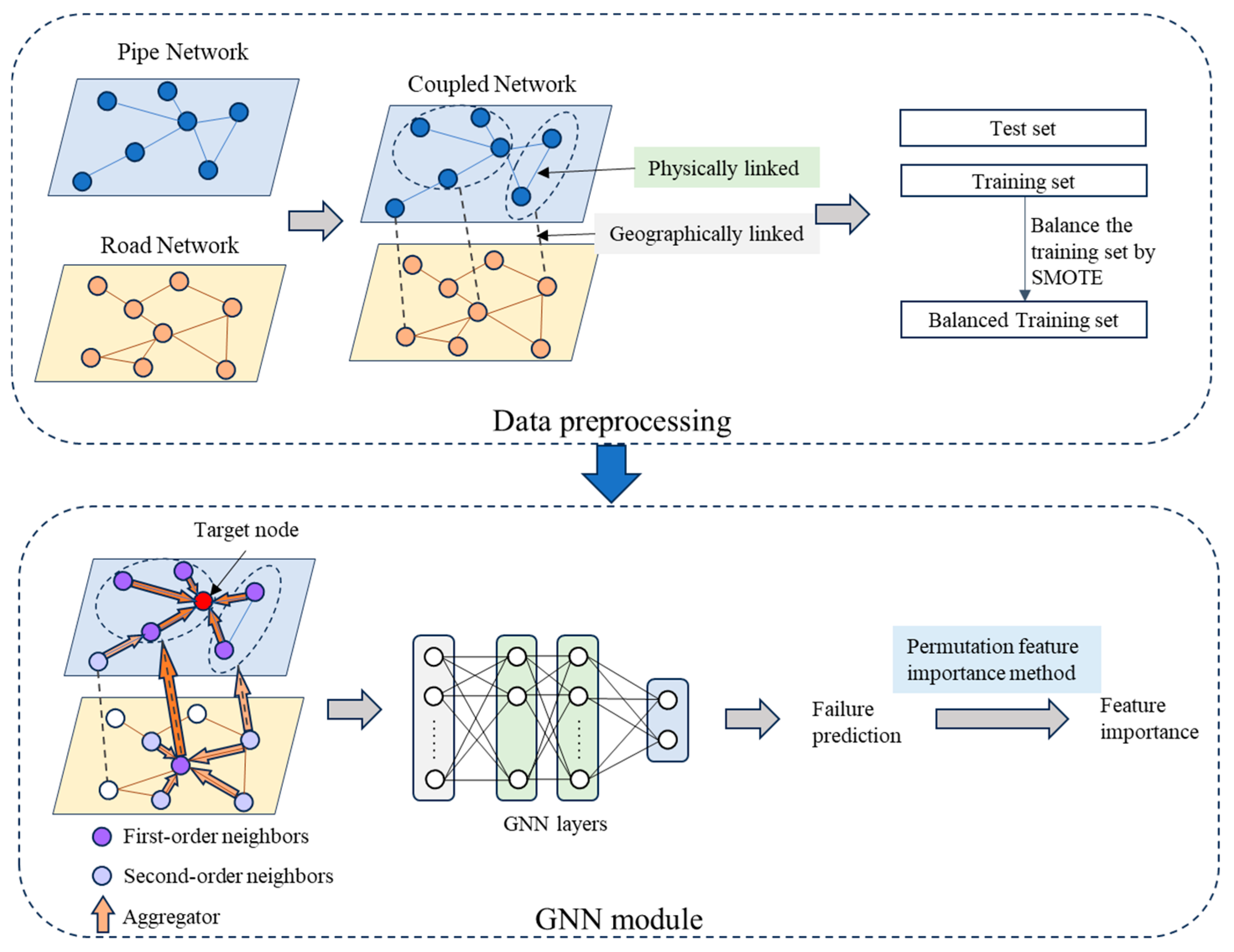
Figure 1 illustrates the complete workflow of our proposed predictive framework. Initially, geographic data and failure records from the local water utility were collected and preprocessed using ArcGIS software to form a structured geographic graph dataset. The resulting dataset was then partitioned into training and testing subsets, with the Synthetic Minority Oversampling Technique (SMOTE) applied to address data imbalance in the training set. Subsequently, several GNN models were trained on the prepared dataset, capturing coupled spatial features from roads and pipelines. Model performances were evaluated using metrics computed on the testing dataset, and permutation feature importance analysis was conducted to quantify the impact of individual features on prediction outcomes.

The following sections provide detailed explanations of each step.

3.2. Data Preprocessing and Feature Engineering

3.2.1. Datasets

The WDN of a specific urban district in Shanghai, China, was selected as the case study area. Data utilized in this study were provided by the local water utility company and included three main types: Geographic Information System (GIS) data for pipelines, GIS data for roads, and historical failure records of pipelines.

Table 1. Overview of the collected datasets.

Data Name	Quantity	Description and Attributes
WDNs GIS Data	38,582	Linear GIS data containing spatial location, pipe length, diameter, pipe age, and burial depth.
Road GIS Data	1086	Linear and areal GIS data containing road names, road grades, road lengths, and spatial boundaries.
Failure Records of WDNs	1200	Failure locations, failure types, pipe material, diameter, installation year, burial depth, length, and repair duration.

summarizes these datasets.

• Pipeline data:
  The pipeline GIS database comprises 38,582 pipe segments with diameters equal to or greater than DN300. Each pipeline record includes spatial coordinates, pipe segment length, pipe diameter, pipe material, burial depth, and installation year.
• Road data:
  The road GIS database contains 1086 road items, including linear (road centerlines) and areal data (road surface boundaries). Roads are classified into four categories according to Chinese national standards [25]: expressways (Class 1), main roads (Class 2), secondary roads (Class 3), and branch roads (Class 4). Each road segment includes attributes such as road grade, road name, and spatial boundaries.
• Failure records:
  The failure dataset comprises 1200 recorded failures from 2002 to 2021, covering a variety of incidents including pipe leakage, corrosion, and pipe bursts, among others. Each failure record includes attributes such as the geographic coordinates of the failure, failure type, repair duration, pipe diameter, pipe material, installation date, burial depth, and pipe length.

The dataset was split into 80% training and 20% testing to ensure a sufficient amount of data for model training while maintaining a representative test set. Given the spatial nature of WDNs and road networks, the data split was performed randomly rather than by geographical region to ensure a balanced distribution of different pipeline attributes in both sets.

3.2.2. Feature Engineering and Encoding Methods

We constructed a geographic graph structure by treating the centroids of pipeline segments and road intersections as graph nodes. For each pipeline segment, features were extracted and engineered based on their intrinsic properties and their spatial relationships with adjacent road structures.

Table 2. Summary of extracted features and encoding methods.

Feature	Encoding	Interpretation
LEN	Continuous	Length of pipeline segment
DCI	Continuous	Distance from pipeline to intersection center
DIA	Continuous	Pipe diameter
AGE	Continuous	Pipe age calculated as the difference between 2021 and year buried
APR	Continuous	Angle between pipeline and road centerline
WIR	Label	Pipeline within road range (0 = no, 1 = yes)
BP	Continuous	Number of connecting pipeline segments at the node
WII	Label	Whether pipeline is within intersection area (0 = no, 1 = yes)
MAT	Label	Pipe material (1 = cast iron, 2 = steel, 3 = ductile cast iron, 4 = polyethylene, 5 = concrete)
DEP	Continuous	Pipe burial depth from road surface
FAL	Continuous	Number of failures before and after defined intervals
RLV	Continuous	Road level of the associated road segment
RLH	Continuous	Highest road grade at intersection
RLL	Continuous	Lowest road grade at intersection
RCT	Continuous	Number of intersecting roads at an intersection
SI	Label	Intersection shape type (1 = X, 2 = Cross, 3 = T, 4 = Y, 5 = Roundabout, 6 = Five or more legs)

provides detailed descriptions of the final features and their encoding methods.

Specifically, pipeline age (AGE) was calculated by subtracting the pipeline installation year from the reference year (2021). The number of pipe segments meeting at a node was counted as branch points (BPs). Road intersections were identified using the intersections of road centerlines, and their geometric shapes were classified into distinct categories based on the number and angles of intersecting roads. Intersections with four roads were categorized into “X” (oblique intersections) and “Cross” (perpendicular intersections). Intersections with three roads were categorized as either “Y” (oblique) or “T” (perpendicular), while intersections involving five or more roads were classified as “Roundabout” or “Five or more legs”, based on their geometric complexity.

Furthermore, spatial analysis using ArcGIS was employed to determine whether pipeline segments fell within road ranges (WIR) and intersection ranges (WII). For segments within roads, the angle between pipelines and road centerlines (APR) was computed. For segments within intersections, the distance from the intersection center (DCI) was calculated.

Table 2 summarizes the extracted features, their encoding methods, and their detailed interpretations. Continuous variables, including pipeline length (LEN), diameter (DIA), pipeline age (AGE), and burial depth (DEP), were directly input into models without further transformation. Categorical variables (MAT, WIR, WII, and SI) were encoded using label encoding, transforming categorical values into numerical labels. For elements not belonging to a certain category (e.g., intersection types for pipeline segments outside intersections), we filled missing entries with a placeholder value of “−1”.

3.3. GNN Module

3.3.1. Overview of GNN Framework

GNNs have shown significant advantages in modeling spatial dependencies within graph-structured data. In this study, we employed several representative GNN models—including GCN, GAT, MixedGNN, DeeperGNN, and GraphSAGE—to predict water distribution network failures. Each model possesses unique strengths in capturing the intricate spatial relationships and interaction patterns inherent in coupled road and pipeline networks. This section briefly introduces these GNN models and their respective characteristics, alongside reasons for their selection in this study context.

3.3.2. GCN

GCN [26] has emerged as a cornerstone in the field of graph-based learning. It generalizes the concept of convolution from grid data to graph data. In GCN, the representation of each node is updated by aggregating the features of its neighboring nodes and itself, followed by a nonlinear transformation. The layer-wise propagation rule can be formulated as follows:

$$H^{(l+1)}=\sigma \left({\tilde{D}}^{-1/2}\tilde{A}{\tilde{D}}^{-1/2}{H}^{\left(l\right)}{W}^{\left(l\right)}\right)$$

(1)

where $H^{\left(l\right)}$ is the matrix of node features at layer l. $\tilde{A}=A+I$ is the adjacency matrix of the graph with added self-loops, $\tilde{D}$ is the degree matrix of $\tilde{A}$, $W^{\left(l\right)}$ is the weight matrix at layer l, and σ is a nonlinear activation function such as ReLU.

The GCN model effectively leverages local structural information and node attributes such as pipe age, diameter, and material, making it particularly suitable for modeling the spatial dependencies influencing network failures.

3.3.3. GAT

GAT [23] introduces an attention mechanism to the graph convolutional networks, allowing nodes to weigh the importance of their neighbors’ features dynamically. The attention coefficients are computed as follows:

$$e_{ij}=\mathrm{LeakyReLU}\left({\mathrm{a}}^T[W{\overrightarrow{h}}_i\mid \mid W{\overrightarrow{h}}_j]\right)$$

(2)

where ${\overrightarrow{h}}_i$ and ${\overrightarrow{h}}_j$ are the feature vectors of nodes i and j, W is a learnable weight matrix, and a is the learnable parameter for the attention mechanism. The operator $\mid \mid$ denotes concatenation, and LeakyReLU is the activation function. The scalar e_ij represents the raw attention score between nodes i and j.

Normalization of attention coefficients are computed as follows:

$${\alpha }_{ij}={\displaystyle \frac{\exp \left(e_{ij}\right)}{\sum _{k\in {\mathcal{N}}_i} \exp \left(e_{ik}\right)}}$$

(3)

In this step, the raw attention scores are normalized using the softmax function to ensure that the sum of attention coefficients for all neighbors of node i equals 1. Here, N_i denotes the set of neighbor nodes of node i.

Feature aggregation is computed as follows:

$${\mathrm{h}}_i^{\prime }=\sigma \left(\sum _{j\in {\mathcal{N}}_i} {\alpha }_{ij}\mathrm{W}{\mathrm{h}}_j\right)$$

(4)

The updated feature vector ${\mathrm{h}}_i^{\prime }$ for node i is obtained by aggregating the weighted features of its neighbors, where σ is a nonlinear activation function, such as ReLU. The weights are determined by the normalized attention coefficients α_ij.

By dynamically assigning different weights to neighboring nodes, GAT effectively highlights crucial areas requiring prioritized maintenance, thus enhancing the accuracy of failure prediction.

3.3.4. MixedGNN (GCN + GAT)

MixedGNN [27] is an innovative architecture that synergistically combines the GCN and GAT models. This hybrid approach allows for the extraction of spatial features through the GCN layers while also utilizing the adaptive attention mechanisms of GAT to focus on the most informative parts of the graph. By integrating both GCN and GAT, MixedGNN is capable of learning richer representations that could enhance the prediction of WDNs failures.

3.3.5. DeeperGNN

DeeperGNN [28] tackles one of the primary challenges in GNNs: the oversmoothing problem that often occurs with deep graph network architectures. DeeperGNN introduces mechanisms to preserve the distinctiveness of node representations in deeper layers of the network. It achieves this through techniques like residual connections, dense connections, or even by learning a unique combination of different propagation depths for each node. These innovations allow DeeperGNN to effectively utilize deep graph structures, making it potentially more accurate for complex tasks like predicting the failure of intricately interconnected water supply systems.

3.3.6. GraphSAGE

GraphSAGE [29] (Graph Sample and AggreGate) is a framework for inductive representation learning on large graphs. It generates node embeddings by sampling and aggregating features from a node’s local neighborhood. The aggregation function can be a mean aggregator, an LSTM aggregator, or a pooling aggregator. The update rule for each node is

$$h_{\mathcal{N}\left(v\right)}^{\left(k\right)}={\mathrm{A}\mathrm{G}\mathrm{G}\mathrm{R}\mathrm{E}\mathrm{G}\mathrm{A}\mathrm{T}\mathrm{E}}_k\left(\right\{h_u^{(k-1)}\mid u\in \mathcal{N}\left(v\right)\left\}\right)$$

(5)

$$h_v^{\left(k\right)}=\sigma (W^k·\mathrm{CONCAT}(h_v^{(k-1)},h_{\mathcal{N}\left(v\right)}^{\left(k\right)}\left)\right)$$

(6)

where $h_v^{\left(k\right)}$ is the feature vector of node v at the k-th layer, N(v) is the set of neighbors of v, and W^k is the weight matrix at layer k.

GraphSAGE is particularly beneficial in our study due to its capability for inductive learning, enabling the model to generalize effectively to unseen nodes and adapt dynamically to changes in network structures, a critical advantage for real-world applications involving evolving WDNs.

By integrating these advanced GNN models, our approach aims to provide a holistic view of the WDN’s health, enabling the early detection and mitigation of potential failures. This predictive capability is crucial for ensuring the reliability and safety of water supply systems, which are vital to public health and urban infrastructure.

3.3.7. Summary of GNN Models

The characteristics, strengths, and limitations of each model are summarized in

Table 3. Summary of GNN models.

Model	Core Principle	Key Advantages	Limitations	Suitability
GCN	Convolutional aggregation	Captures local graph structures	Less effective for distant nodes	Static spatial dependencies
GAT	Attention-based aggregation	Adaptive weighting of neighbors	Computationally intensive	Important localized dependencies
MixedGNN	Hybrid (GCN+GAT)	Combines spatial and attention features	Increased model complexity	Balanced local- global relationships
DeeperGNN	Deep structure with smoothing control	Maintains deep representation distinctiveness	Complex training and hyperparameter tuning	Complex, dense graph structures
GraphSAGE	Inductive learning via sampling	Good scalability, inductive learning	Dependent on sampling quality	Large-scale, dynamic graphs

, providing a clear rationale for model selection based on our prediction task’s specific needs.

3.4. Model Implementation and Evaluation

3.4.1. Overview of Model Implementation

Algorithm 1 outlines the structured implementation of the proposed GNN-based failure prediction model, detailing key steps from data processing to model evaluation. Initially, the programming environment was configured, followed by the preparation of raw spatial data for subsequent feature extraction. Feature processing and encoding were then performed to integrate relevant attributes, constructing a comprehensive geographic graph dataset. To mitigate data imbalance, SMOTE resampling was applied before defining and training the GNN models, which were subsequently evaluated on a separate test set.

Algorithm 1 GNN-based failure prediction model.

Input: Spatial and attribute data D

Output: Trained GNN model M with evaluated feature importance

Step 1: Load and preprocess data

Load spatial and attribute data D from ArcGIS

Merge pipeline and road network attributes into structured dataframes

Step 2: Construct geographic graph

Initialize graph G = (V, E) using NetworkX

for each pipeline segment and road intersection i ∈ D do

Add node vi with extracted features

Add edges E based on spatial connectivity

end for

Step 3: Apply data balancing (SMOTE)

Apply SMOTE to generate synthetic samples for minority class

Integrate resampled data into graph G

Step 4: Define and train GNN models

for each GNN model Mk ∈ {GCN, GAT, GraphSAGE, MixedGNN, DeeperGNN}

do

Initialize model architecture Mk

Train Mk using AdamW optimizer and Focal Loss

Evaluate Mk using AUC-ROC, accuracy, and recall

end for

Step 5: Perform feature importance analysis

for each feature fj in feature set do

Permute values of fj

Compute impact on model performance ΔAUC

end for

Return: Trained model M and feature importance scores

3.4.2. Programming Environment and Data Preparation

All modeling tasks in this study were performed using Python (version 3.8.8). Key libraries included pandas (version 1.2.4) for data manipulation, NetworkX (version 2.6) for geographic graph construction, PyTorch (version 2.1.2) and PyTorch Geometric (version 2.4.0) for building and training graph neural networks, and scikit-learn (version 1.3.2) for data preprocessing and evaluation.

Initially, attribute tables and spatial coordinate data for pipelines, intersections, and road segments were exported from ArcGIS into Excel spreadsheets. These data files were loaded into Python using pandas and systematically organized into structured dataframes, ensuring consistency for subsequent analysis. Specifically, pipeline attributes such as length, diameter, age, and failure history were merged with spatial coordinates. Similarly, road intersection and segment data integrated attributes like intersection shape and road grades, creating a unified dataset for graph construction.

3.4.3. Graph Construction and Feature Engineering

A geographic graph structure was constructed using NetworkX. Nodes represented the centroids of pipeline segments and road intersections, and edges denoted their spatial and functional connections.

Feature extraction was performed to capture critical spatial and infrastructural characteristics influencing pipeline failures. Extracted features included intrinsic pipeline properties (e.g., diameter, age, burial depth) and spatial interactions with road networks, such as angles between pipelines and roads (APR), pipeline segments within road ranges (WIR), and intersections (WII). Distances and angles were calculated using ArcGIS’s azimuth and distance measurement functions. Intersection types were classified based on geometric configurations of intersecting roads as previously detailed.

Extracted attributes were consolidated into comprehensive, uniform feature vectors for all graph nodes. Continuous variables like pipeline length, diameter, pipe age, and burial depth were directly integrated. Categorical features (material type, intersection shape, inclusion within roads/intersections) were numerically encoded using label encoding. Missing categorical values were systematically filled with placeholder values (−1) to maintain data consistency.

3.4.4. Data Balancing and Resampling

To effectively address class imbalance within the dataset, the SMOTE [30] was applied. SMOTE generates synthetic minority-class instances, creating a balanced dataset crucial for accurate model training and reliable prediction outcomes. The balanced dataset was then updated and integrated into the previously constructed geographic graph, preparing it for subsequent model training.

3.4.5. Model Definition, Training, and Evaluation

Multiple Graph Neural Network models, including GCN, GAT, MixedGNN, DeeperGNN, and GraphSAGE, were defined and implemented using PyTorch and PyTorch Geometric libraries. Each model was designed to optimize feature extraction while maintaining computational efficiency. Model training was conducted using the AdamW optimizer, combined with a learning rate scheduler to dynamically adjust learning rates during training. Focal loss [31] was selected as the loss function to mitigate the impact of class imbalance by prioritizing harder-to-classify examples, thus improving overall predictive performance.

To mitigate overfitting, we employed several regularization techniques. Dropout layers were used in the GNN models, and L2 weight decay was applied to prevent excessive model complexity. Additionally, early stopping was implemented based on validation loss to avoid overfitting. The training dataset was balanced using SMOTE to enhance the robustness of the model against imbalanced data.

To ensure optimal performance, we fine-tuned the hyperparameters of the GNN models through an extensive grid search. The final set of control parameters used in our study is summarized as follows:

• Learning rate: 0.001. This value was chosen to balance convergence speed and stability, preventing the model from becoming stuck in local minima or diverging.
• Batch size: 64. A moderate batch size was selected to maintain efficient computation while ensuring stable gradient updates.
• Dropout rate: 0.2. Applied to prevent overfitting by randomly deactivating neurons during training.
• Number of hidden layers: 3. Based on empirical results, a three-layer architecture effectively captured hierarchical graph dependencies while avoiding oversmoothing.
• Optimizer: AdamW. Adam with weight decay was selected due to its adaptive learning rate and superior performance in graph-based tasks.
• Loss function: Focal loss. Given the class imbalance in pipeline failure data, focal loss was employed to down-weight easy-to-classify samples and emphasize harder examples, improving recall. A focusing parameter of γ = 2 was applied based on empirical tuning.
• GraphSAGE aggregation type: Mean aggregator. This choice ensures effective information propagation from neighboring nodes while maintaining computational efficiency.

Additionally, we implemented early stopping with a patience of 10 epochs to prevent overfitting. The model training was performed for a maximum of 200 epochs, with checkpointing based on validation loss. Hyperparameter tuning was conducted using cross-validation to ensure the robustness of the selected parameters.

To quantitatively evaluate the performance of our predictive models, we employed the following statistical metrics:

• Accuracy (ACC)

$$ACC={\displaystyle \frac{TP+TN}{TP+TN+FP+FN}}$$

(7)

where TP (true positives) and TN (true negatives) represent correctly classified instances, while FP (false positives) and FN (false negatives) denote misclassified instances.

• Precision (P)

$$P={\displaystyle \frac{TP}{TP+FP}}$$

(8)

Precision measures the proportion of correctly predicted positive instances out of all predicted positive cases.

• Recall (R)

$$R={\displaystyle \frac{TP}{TP+FN}}$$

(9)

Recall indicates the proportion of actual positive instances correctly identified.

• F1-score (F1)

$$F1=2\times {\displaystyle \frac{P\times R}{P+R}}$$

(10)

F1-score is the harmonic mean of precision and recall, balancing the trade-off between them.

• Area under the curve—receiver operating characteristic (AUC-ROC)

AUC-ROC evaluates the model’s ability to distinguish between positive and negative cases. It is computed as the area under the ROC curve, where a higher AUC indicates superior model performance.

The primary evaluation metric used in this study is AUC-ROC, as it provides a threshold-independent assessment of model performance. Unlike accuracy, recall, and F1-score, which are influenced by the choice of classification threshold, AUC measures the model’s ability to distinguish between positive and negative cases across all possible thresholds. This makes it a more robust indicator for imbalanced classification problems, such as pipeline failure prediction, where the choice of threshold can significantly impact other metrics. While we also report accuracy and recall for additional insights, their values depend on the selected classification threshold. The optimal threshold for deployment in real-world applications can be determined based on operational requirements, such as minimizing false negatives in failure detection

3.4.6. Permutation-Based Feature Importance Estimation

To further interpret model predictions and understand the contribution of individual features, permutation feature importance analysis [32] was performed. This method assesses feature significance by measuring prediction performance degradation upon randomly permuting individual feature values. Specifically, the original performance metric AUC was compared against the metric obtained after permuting each feature. The difference between these two metrics quantifies the importance of each feature, thereby identifying critical predictors influencing pipeline failure predictions. Furthermore, to evaluate the importance of network topology information into failure prediction, we introduced the topological feature (TOP) by measuring the change in AUC before and after removing all edges between supply network nodes.

4. Results and Discussion

4.1. Model Performance Evaluation

The training was conducted on a PC equipped with an Intel Core i9 processor with 32.0 GB of RAM, and an NVIDIA Quadro RTX 3000 graphics card was used to accelerate the computation. To evaluate the performance of different models in predicting water pipeline failures, we compared traditional machine learning models (random forest, SVM, ANN) with various GNN architectures. The results, presented in

Table 4. Results of GNNs and other models.

Model	AUC	Accuracy	Recall	Precision	F1-Score
Random Forest	0.731	0.591	0.724	0.037	0.070
SVM	0.722	0.623	0.723	0.031	0.059
ANN	0.760	0.638	0.781	0.046	0.087
GCN	0.738	0.744	0.590	0.042	0.078
GAT	0.806	0.761	0.636	0.053	0.098
MixedGNN	0.805	0.662	0.773	0.056	0.104
DeeperGNN	0.817	0.693	0.818	0.059	0.110
GraphSAGE	0.821	0.712	0.878	0.067	0.125

, illustrate the predictive capability of each model in terms of AUC, accuracy, recall, precision, and F1-score.

Generally, a model with an AUC above 0.80 is considered to have good predictive ability [13,33]. Therefore, GAT, MixedGNN, DeeperGNN, and GraphSAGE can all be considered good predictive models. Among all models, GraphSAGE achieved the best overall performance, with an AUC of 0.821, recall of 0.878, and F1-score of 0.125, demonstrating its effectiveness in modeling spatial dependencies in WDNs. DeeperGNN also performed well, with an AUC of 0.817, benefiting from deeper feature extraction while avoiding the oversmoothing issue common in graph-based models.

These results indicate that GNN-based models significantly outperform traditional machine learning approaches. GraphSAGE and DeeperGNN exhibited superior recall values, demonstrating strong predictive capabilities for detecting potential pipeline failures. This finding aligns with the conclusions of Liang et al. [34] (2021), who found that GNN models outperform classical ML models in urban infrastructure failure predictions due to their ability to capture spatial dependencies.

The superior performance of GraphSAGE can be attributed to its ability to aggregate node neighborhood information effectively while preserving key structural dependencies. Unlike traditional convolutional models like GCN, which suffer from information dilution across layers, GraphSAGE employs an inductive learning mechanism that dynamically samples and aggregates node features, leading to more robust generalization. The attention-based GAT model also demonstrated competitive performance (AUC = 0.806), benefiting from its capability to assign different importance levels to neighboring nodes. However, its computational complexity is higher compared to GraphSAGE, making it less scalable for large-scale infrastructure networks.

While traditional ML models (RF, SVM, ANN) achieved moderate accuracy, they struggled to capture the spatial and topological dependencies inherent in WDNs. The random forest and SVM models showed lower AUC values (0.731 and 0.722, respectively), likely due to their inability to leverage spatial relationships between pipeline segments and road networks.

However, all models displayed relatively low precision and F1-score values. Such low precision is commonly encountered in pipeline failure predictions due to severe class imbalance—failed pipes represent only a very small fraction of the dataset. As emphasized by Liu et al. [13] (2023), false positives identified by the models might still represent pipes at an increased risk of future failure, thus justifying proactive monitoring or early intervention. Hence, relying solely on precision as a performance metric may underestimate a model’s true operational value. To better evaluate the practical effectiveness of the predictive models, the next section introduces the concept of failure detection rate [34], focusing on the practical utility of these models for prioritizing maintenance activities.

4.2. Failure Detection Rate Analysis

Considering that the predictive models yielded relatively low precision values, it is important to evaluate their effectiveness from a practical maintenance perspective. In real-world scenarios, the proactive maintenance of water distribution networks involves high financial and labor costs, making it impractical to inspect all pipes comprehensively. Therefore, the practical goal of failure prediction is not merely to achieve high precision, but to accurately rank and prioritize pipes according to their failure risk.

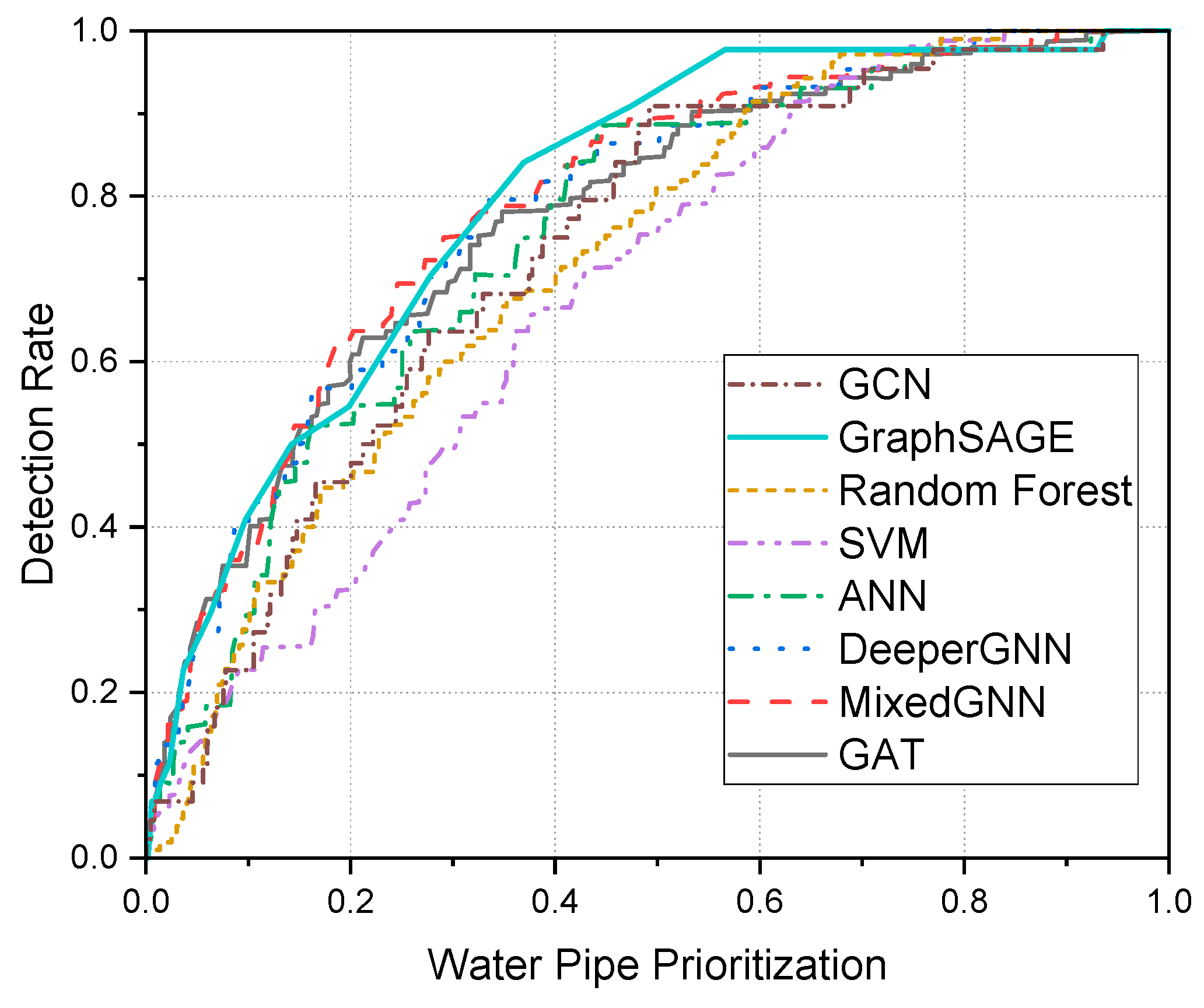
Following this logic, we further evaluated our models using the detection rate at top ranking predictions for WDNs. As shown in Figure 2, our predictive model effectively identified high-risk pipes, for example, the GraphSAGE model identified more than 50% of the actual failures detected by inspecting only the top 13.5% of ranked pipes; over 75% of failures were captured within the top 31.6%; and, notably, more than 98% of the failures could be found by inspecting just the top 53.6% of pipes.

These findings underscore the practical value of our predictive framework. Despite low precision metrics, the model effectively identifies high-risk pipes, thereby significantly optimizing maintenance efforts and resource allocation. By prioritizing inspections according to model predictions, utility operators can proactively mitigate risks, enhance network reliability, and reduce overall operational costs. To further enhance preventive maintenance, the utility should increase the frequency of inspections for pipes predicted to fail and install sensors to monitor the condition of these pipes in real time.

4.3. Interpretation of Key Features in Failure Prediction

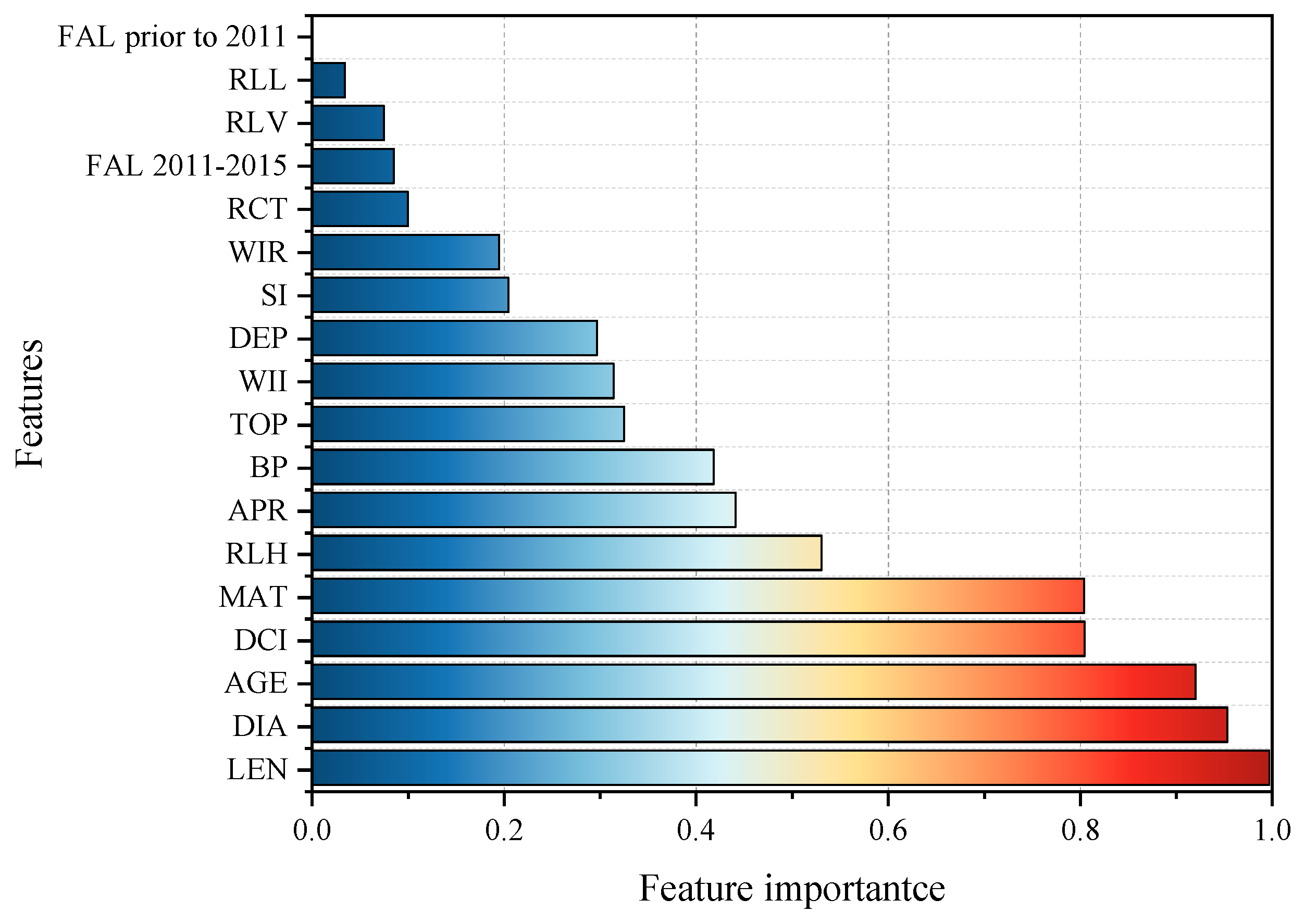
To further understand the key factors influencing pipeline failures and to refine our predictive model, we conducted a feature importance analysis using the permutation feature importance method. The results are presented in Figure 3, which ranks the most significant factors affecting pipeline failures.

The feature importance analysis underscores the critical role of intrinsic pipeline attributes—LEN, DIA, AGE, and MAT—consistent with prior research [13,34,35]. These attributes are widely recognized as fundamental determinants of pipeline deterioration, as longer pipes have more potential failure points, aging pipes degrade structurally over time, and smaller-diameter pipes are more vulnerable to internal pressure fluctuations and external mechanical stress.

Beyond these well-known characteristics, our analysis highlights the impact of road–infrastructure coupling factors and topological network features. Among them, DCI, MAT, and APR emerge as significant contributors to failure risk. The influence of DCI and APR suggests that traffic-related transverse and higher dynamic loads near intersections are critical external factors affecting pipeline integrity, aligning with previous studies [36]. The strong influences of DCI and APR suggest that conventional pipeline failure prediction models may underestimate the impact of road traffic conditions on failure risk. Traditional models primarily focus on pipe material, age, and diameter, but our findings indicate that road-induced mechanical stress significantly contributes to failure likelihood. These results suggest that future predictive frameworks should integrate coupled road–pipeline attributes to improve accuracy, an area that has received limited attention in prior research.

Both TOP and BP significantly contribute to model performance, emphasizing the importance of network structural dependencies in failure risk assessment. As introduced in Section 3.4.5, TOP quantifies the connectivity of the pipeline network, capturing how pipelines interact within the broader system, confirming that GNN-based models leverage topological information to enhance predictive accuracy. Similarly, BP represents the local network structure, capturing both pipeline junction complexity and the structural vulnerabilities of joints. Studies have shown that most pipeline damage occurs at joints under traffic-induced stress [37], supporting BP as an indicator of structural weakness. As a result, pipelines in high-BP regions should be prioritized for monitoring and maintenance, particularly in areas subject to heavy external loads. The strong influence of TOP and BP highlights the necessity of incorporating global and local network structure into failure prediction models, moving beyond traditional approaches that focus solely on isolated pipeline characteristics.

Furthermore, while historical failure rates (FAL) were initially expected to be a strong predictor, our analysis shows that they have relatively low importance. This may be due to variations in past repair strategies—some pipelines were fully replaced after failure, reducing their probability of subsequent failures, while others were only partially repaired, retaining their vulnerability. This finding underscores the importance of integrating maintenance history details into predictive models to refine failure risk assessments.

By incorporating both physical attributes and network structure dependencies, our results suggest that failure prediction models can be further improved by accounting for how pipelines interact with the broader network and external road conditions. These findings emphasize the necessity of moving beyond traditional material-based failure models to develop more resilient and data-driven risk assessment frameworks.

5. Conclusions

This study addressed the limitations of traditional machine learning models by integrating coupled road–pipeline network features into GNN-based failure prediction. The results demonstrate that GNN models, particularly GraphSAGE and DeeperGNN, effectively capture complex spatial dependencies, significantly improving predictive accuracy. Among these, GraphSAGE exhibited the highest performance, highlighting its potential for practical applications in infrastructure risk assessment. Major conclusions include the following:

• Innovative traffic-related indicators enhance predictive capabilities. By explicitly incorporating road infrastructure and traffic-related factors into failure prediction models, this study improves the accuracy and reliability of pipeline failure risk assessments. Key coupled features, such as intersection proximity and pipeline–road angles, were found to significantly influence failure risk.
• Comparative evaluation of GNN architectures provides insights into infrastructure resilience modeling. The performance of different GNN models was systematically assessed, demonstrating that GraphSAGE and DeeperGNN outperform traditional ML approaches by capturing spatial dependencies more effectively. This evaluation fills a gap in the literature by identifying the most suitable GNN architectures for urban pipeline failure prediction.
• Coupled network topological features play a crucial role in predictive models. The study validates the importance of incorporating spatial dependencies, showing that topological attributes significantly contribute to failure risk prediction. The integration of network topology features enhances the model’s ability to assess vulnerabilities in urban infrastructure systems.

Despite these contributions, several limitations remain. First, the model exhibits relatively low precision, leading to a higher false positive rate, which may reduce its practical applicability. Second, the dataset lacks post-failure intervention details, making it difficult to account for how repairs or replacements influence future failures. Finally, while this study captures spatial dependencies, it does not explicitly consider temporal dynamics, which could further refine failure predictions.

To address these limitations, future work should focus on improving model precision by optimizing classification thresholds and integrating uncertainty quantification techniques. Expanding datasets to include post-failure intervention records will enhance prediction reliability. Additionally, incorporating temporal and environmental factors—such as seasonal variations, soil conditions, and pressure fluctuations—can further improve model robustness. Finally, validation through real-world case studies and field experiments will be essential for assessing the practical implementation of these models in urban infrastructure management. By addressing these challenges, future research can contribute to more effective failure prediction frameworks, supporting proactive maintenance strategies and enhancing urban infrastructure resilience.

References

- Statistics, National Bureau of Statistics. National Bureau of Statistics of China. Available online: https://www.stats.gov.cn/ (accessed on 19 March 2025).
- Robert, D.J.; Chan, D.; Rajeev, P.; Kodikara, J. Effects of operational loads on buried water pipes using field tests. Tunn. Undergr. Space Technol. 2022, 124, 104463. [Google Scholar] [CrossRef]
- Li, B.; Guo, X.X.; Fang, H.Y.; Ren, J.L.; Yang, K.J.; Wang, F.; Tan, P.L. Prediction equation for maximum stress of concrete drainage pipelines subjected to various damages and complex service conditions. Constr. Build. Mater. 2020, 264, 120238. [Google Scholar] [CrossRef]
- Li, B.; Fang, H.; He, H.; Yang, K.; Chen, C.; Wang, F. Numerical simulation and full-scale test on dynamic response of corroded concrete pipelines under Multi-field coupling. Constr. Build. Mater. 2019, 200, 368–386. [Google Scholar] [CrossRef]
- Xi, Z.S.; Ying, W.; Wei, J.P. Reliability analysis of buried polyethylene pipeline subject to traffic loads. Adv. Mech. Eng. 2019, 11, 1687814019883785. [Google Scholar] [CrossRef]
- Underground Pipeline Committee of China Association of City Planning. Statistical Analysis Report of Underground Pipeline Accidents in China in 2021; CACP: Beijing, China, 2022.
- Rajani, B.; Kleiner, Y. Comprehensive review of structural deterioration of water mains: Physically based models. Urban Water 2001, 3, 151–164. [Google Scholar] [CrossRef]
- Kleiner, Y.; Rajani, B. Comprehensive review of structural deterioration of water mains: Statistical models. Urban Water 2001, 3, 131–150. [Google Scholar] [CrossRef]
- Chen, R.; Wang, Q.; Javanmardi, A. A Review of the Application of Machine Learning for Pipeline Integrity Predictive Analysis in Water Distribution Networks. Arch. Comput. Methods Eng. 2025, 32, 1–29. [Google Scholar] [CrossRef]
- Shirzad, A.; Tabesh, M.; Farmani, R. A comparison between performance of support vector regression and artificial neural network in prediction of pipe burst rate in water distribution networks. KSCE J. Civ. Eng. 2014, 18, 941–948. [Google Scholar] [CrossRef]
- Kakoudakis, K.; Farmani, R.; Butler, D. Pipeline failure prediction in water distribution networks using weather conditions as explanatory factors. J. Hydroinformatics 2018, 20, 1191–1200. [Google Scholar] [CrossRef]
- Robles-Velasco, A.; Ramos-Salgado, C.; Muñuzuri, J.; Cortés, P. Artificial Neural Networks to Forecast Failures in Water Supply Pipes. Sustainability 2021, 13, 8226. [Google Scholar] [CrossRef]
- Liu, W.; Xie, Z.; Song, Z. Predicting Water Pipe Failures Using Deep Learning Algorithms. J. Infrastruct. Syst. 2023, 29, 04023022. [Google Scholar] [CrossRef]
- Cen, H.; Huang, D.; Liu, Q.; Zong, Z.; Tang, A. Application Research on Risk Assessment of Municipal Pipeline Network Based on Random Forest Machine Learning Algorithm. Water 2023, 15, 1964. [Google Scholar] [CrossRef]
- Fan, X.; Wang, X.; Zhang, X.; Yu, X. Machine learning based water pipe failure prediction: The effects of engineering, geology, climate and socio-economic factors. Reliab. Eng. Syst. Saf. 2022, 219, 108185. [Google Scholar] [CrossRef]
- Elshaboury, N.; Abdelkader, E.M.; Al-Sakkaf, A.; Alfalah, G. Teaching-Learning-Based Optimization of Neural Networks for Water Supply Pipe Condition Prediction. Water 2021, 13, 3546. [Google Scholar] [CrossRef]
- Lopez, L.L.; van Zyl, J.E.; Harkness, B. Analysis and Modeling of Pressure Pipe Failures in Auckland, New Zealand. J. Water Resour. Plan. Manag. 2024, 150, 04024007. [Google Scholar] [CrossRef]
- Snider, B.; McBean, E.A. Improving urban water security through pipe-break prediction models: Machine learning or survival analysis. J. Environ. Eng. 2020, 146, 04019129. [Google Scholar] [CrossRef]
- Zhang, J.; Gu, X.; Zhou, Y.; Wang, Y.; Zhang, H.; Zhang, Y. Mechanical Properties of Buried Gas Pipeline under Traffic Loads. Processes 2023, 11, 3087. [Google Scholar] [CrossRef]
- Sun, M.-M.; Fang, H.-Y.; Wang, N.-N.; Du, X.-M.; Zhao, H.-S.; Zhai, K.-J. Limit state equation and failure pressure prediction model of pipeline with complex loading. Nat. Commun. 2024, 15, 4473. [Google Scholar] [CrossRef]
- Peng, R.; Wang, G.; Li, S.; Qiao, Q.; Wang, Y.; Xu, Z. Fatigue assessment of buried metal pipelines under traffic loads using video monitoring data. Struct. Health Monit. 2023, 22, 3385–3400. [Google Scholar] [CrossRef]
- Jin, G.; Liang, Y.; Fang, Y.; Shao, Z.; Huang, J.; Zhang, J.; Zheng, Y. Spatio-temporal graph neural networks for predictive learning in urban computing: A survey. IEEE Trans. Knowl. Data Eng. 2023, 36, 5388–5408. [Google Scholar] [CrossRef]
- Velickovic, P.; Cucurull, G.; Casanova, A.; Romero, A.; Lio’, P.; Bengio, Y. Graph Attention Networks. arXiv 2017, arXiv:1710.10903. [Google Scholar]
- Xu, Y.; He, Z. Pipe Failure Prediction in the Water Distribution System Using a Deep Graph Convolutional Network and Temporal Failure Series. ACS EST Eng. 2024, 4, 2252–2262. [Google Scholar] [CrossRef]
- CJJ37-2012; Code for Urban Road Engineering Design. Ministry of Housing and Urban-Rural Development of the People’s Republic of China: Beijing, China, 2016.
- Zhang, H.; Lu, G.; Zhan, M.; Zhang, B. Semi-Supervised Classification of Graph Convolutional Networks with Laplacian Rank Constraints. Neural Process. Lett. 2022, 54, 2645–2656. [Google Scholar] [CrossRef]
- Gorka, J.; Hsu, T.; Li, W.; Maximov, Y.; Roald, L. Cascading blackout severity prediction with statistically-augmented graph neural networks. Electr. Power Syst. Res. 2024, 234, 110738. [Google Scholar] [CrossRef]
- Li, G.; Xiong, C.; Thabet, A.; Ghanem, B. DeeperGCN: All You Need to Train Deeper GCNs. arXiv 2020, arXiv:2006.07739. [Google Scholar]
- Huang, K.; Chen, C. Subgraph generation applied in GraphSAGE deal with imbalanced node classification. Soft Comput. 2024, 28, 10727–10740. [Google Scholar] [CrossRef]
- Fernández, A.; Garcia, S.; Herrera, F.; Chawla, N.V. SMOTE for learning from imbalanced data: Progress and challenges, marking the 15-year anniversary. J. Artif. Intell. Res. 2018, 61, 863–905. [Google Scholar] [CrossRef]
- Lin, T.Y.; Goyal, P.; Girshick, R.; He, K.; Dollár, P. Focal Loss for Dense Object Detection. In Proceedings of the 2017 IEEE International Conference on Computer Vision (ICCV), Venice, Italy, 22–29 October 2017; pp. 2999–3007. [Google Scholar]
- Altmann, A.; Toloşi, L.; Sander, O.; Lengauer, T. Permutation importance: A corrected feature importance measure. Bioinformatics 2010, 26, 1340–1347. [Google Scholar] [CrossRef] [PubMed]
- Xu, H.; Sinha, S. Modeling Pipe Break Data Using Survival Analysis with Machine Learning Imputation Methods. J. Perform. Constr. Facil. 2021, 35, 04021071. [Google Scholar] [CrossRef]
- Liang, S.; Li, Z.; Liang, B.; Ding, Y.; Wang, Y.; Chen, F. Failure Prediction for Large-scale Water Pipe Networks Using GNN and Temporal Failure Series. In Proceedings of the 30th ACM International Conference on Information & Knowledge Management Virtual Event, Queensland, Australia, 1–5 November 2021; pp. 3955–3964. [Google Scholar]
- Liu, W.; Wang, B.H.; Song, Z.Y. Failure Prediction of Municipal Water Pipes Using Machine Learning Algorithms. Water Resour. Manag. 2022, 36, 1271–1285. [Google Scholar] [CrossRef]
- Wu, T.; Yu, H.; Jiang, N.; Zhou, C.; Luo, X. Theoretical analysis of the deformation for steel gas pipes taking into account shear effects under surface explosion loads. Sci. Rep. 2022, 12, 8658. [Google Scholar] [CrossRef] [PubMed]
- Xu, M. Article Centrifuge testing to simulate buried reinforced concrete pipe joints subjected to traffic loading. Can. Geotech. J. 2015, 52, 1762–1774. [Google Scholar] [CrossRef]
Disclaimer/Publisher’s Note: The statements, opinions and data contained in all publications are solely those of the individual author(s) and contributor(s) and not of MDPI and/or the editor(s). MDPI and/or the editor(s) disclaim responsibility for any injury to people or property resulting from any ideas, methods, instructions or products referred to in the content. |
© 2025 by the authors. Licensee MDPI, Basel, Switzerland. This article is an open access article distributed under the terms and conditions of the Creative Commons Attribution (CC BY) license (https://creativecommons.org/licenses/by/4.0/).