Abstract
This study explores the relationships between environmental factors and the distribution of epilithic diatoms in 161 estuaries of three coastal areas on the Korean peninsula. We investigated epilithic diatoms, water quality, and land use in the vicinities of the estuaries during the months of May 2012, 2013 and 2014, because Korea is relatively free from the influences of rainfall at that time of year. We recorded 327 diatom taxa from the study sites, and the assemblage was dominated by members of the Naviculaceae. Bacillariaceae accounted for the largest proportion of diatoms, and Nitzschia inconspicua (18%) and N. frustulum (9.6%) were the most dominant species. A cluster analysis based on epilithic diatom abundance suggested that the epilithic diatom communities of Korean estuaries can be classified into four large groups (G) according to geography, as follows: Ia—the East Sea watershed, Ib—the eastern watershed of the South Sea, IIa—the West Sea watershed, and IIb—the western watershed of the South Sea. The former two groups, Ia and Ib, showed higher proportions of forest land cover and use, higher species occurrence, lower salinity, lower turbidity, and lower concentrations of nutrients than the latter two groups, while the latter groups, IIa and IIb, had higher proportions of agricultural land cover and use, higher electrical conductivity, higher turbidity, higher concentrations of nutrients, and lower species occurrence. The environmental factors underlying the distribution of epilithic diatoms, representative of each region, are as follows: dissolved oxygen and forest land cover and use for Reimeria sinuate and Rhoicosphenia abbreviate of the East Sea (ES), salinity and turbidity for Tabularia fasciculate of the West Sea (WS), and biochemical oxygen demand (BOD) and nutrients for Cyclotella meneghiniana of the WS. On the other hand, the most influential environmental factors affecting the occurrence of indicator species showing the highest indicator values (>60%) of each group were electrical conductivity for Navicula saprophila and Reimeria sinuate of Ia, and turbidity for Encyonema minutum of IIa. Collectively, the distribution of epilithic diatom communities inhabiting Korean estuaries are determined by geographical factors and water quality, which are in turn influenced by land cover and use, and which differ from east to west.
1. Introduction
The Korean peninsula is surrounded by seas, and these seas can be divided into two parts (the West and South Seas and the East Sea). The West and South Seas (WS and SS) are characterized by indented coastlines, large tidal ranges, and well-developed tidal flats. The East Sea (ES) is marked by high mountain ranges, high water levels, simple coastlines, and higher water quality. Despite its limited land area, there are more than 500 estuaries of different sizes on the Korean peninsula. Generally, there are two types of estuaries, including enclosed estuaries, which shut off the influx of seawater with artificial structures, and open estuaries, which occur without such structures [1]. Recently, structures such as dams and irrigation reservoirs have been built in the West Sea and South Sea areas, leading to a gradual increase in the number of enclosed estuaries on the Korean peninsula [2].
According to geographical aspects and environmental management of the watershed regions, Korean estuaries can be divided into seven areas. The seven areas include the West Han River, the East Han River, the Geum River, the Yeongsan River, the Seomjin River, the Nakdong River, and Jeju Island [3]. The watershed regions of estuaries in Korea consist of forest (39.2%), agricultural land (28.8%), bodies of water (16.4%), and cities (5.8%). Among the seven areas of estuaries, the East Han River area, a region spanning the Han River to the East Sea, is largely dominated by forest area (78%) and agricultural land (11%). In contrast, the Geum River area and the Yeongsan River area have higher proportions of urban and agricultural land due to national reclamation and land development projects of the Korean government [3].
Estuaries are transition zones where freshwater joins seawater, and are dynamic systems where volatile physicochemical changes occur in water temperature, salinity, and nutrients [4,5]. Not only are estuaries valued from an ecological perspective as habitats in which a variety of organisms live, nurture, and spawn, but estuaries are also valued from a socio-economical perspective for agriculture, transportation, tourism, and leisure activities [6,7,8]. However, the growth of cities within estuary basins has resulted in a population boom in Korea. What is more, the development of estuaries and diverse industrial facilities is associated with the destruction of natural environments and ecosystems in estuaries, with subsequent influxes of domestic and industrial wastewater and sewage causing environmental problems [9,10]. Such problems are more marked in enclosed estuaries [1,11,12].
Together with bacteria, diatom communities are major biological factors producing biofilms on various underwater substrates [13]. Like phytoplankton and aquatic plants, diatoms are an important primary producer in aquatic food webs and energy flows, as well as a food source for large invertebrates and fish communities [14,15,16]. In addition, diatoms respond more quickly than other biota (macro-invertebrates and fish communities) to physicochemical changes in photo-intensity, water temperature, salinity, and nutrients, not only in freshwater but also in seawater [17,18]. That is why diatom communities can be used to explain the influences of seawater and water temperature on microalgae communities in both enclosed and open estuaries [19,20,21,22,23,24,25]. In particular, due to their low mobility, epilithic diatom communities have long been used to estimate the cumulative effects of pollutants over long periods of time, and to predict the occurrence and abundance of upstream regulators [26,27,28,29]. Streams have attracted attention as lotic water zones used by investigators to explore factors influencing the distribution of epilithic diatoms, such as landscape, weather, land use/cover, and hydrologic conditions [30,31,32,33].
There is much room for further research on the influence of water quality on epilithic diatom communities and the relationships between the distribution of diatom communities and the environment at both domestic and global scales. The water quality of Korean estuaries and their biological communities, including the phytoplankton, vegetation structures, fish communities, and macro-invertebrates, are frequently studied [34,35,36,37]. However, prior research efforts have focused on the nutrients flowing into streams or eutrophication and the red tides caused by fish farming businesses within estuary basins [38,39,40,41]. Consequently, there has not been adequate research on epilithic diatom communities in estuaries. In addition, considering that freshwater and seawater mix cyclically in estuaries, investigating the conditions of aquatic ecosystems based on highly mobile phytoplankton, macro-invertebrates, and fish communities is a very limited approach in terms of time and space [42,43]. Also observed in estuaries are lower degrees of complexity and sinuosity than in upper streams and rivers, and thus, simple microhabitats (river beds and canopy) allow more accurate interpretations of environments in which sessile organisms with limited mobility accumulate [44,45]. Therefore, to fully understand Korean estuaries with their large variation in geographical features and size, epilithic diatom communities and environmental factors must be studied.
This study aims to assess the relationships between epilithic diatom communities and environmental factors in 90 highly accessible streams (161 study sites) distributed among all the estuaries in the Korean peninsula during a period that is relatively insensitive to rainfall. Our goals were (i) to characterize the distributional patterns of epilithic diatom communities in estuaries in the Korean peninsula and ii) to evaluate the effects of environmental factors on the distribution and occurrence of epilithic diatom communities in Korean estuaries.
2. Materials and Methods
2.1. Ecological Data
This survey was conducted in five watershed regions (161 study sites among 90 estuaries), not including poorly accessible areas such as the West Han River and Jeju Island, during the months of May in 2012, 2013 and 2014 (May is a period that is less influenced by rainfall than the rest of the year). For convenience, the survey areas were analyzed in the following order: the East Sea watershed (45 sites), the South Sea watershed (81 sites), and the West Sea watershed (35 sites) (Figure 1). In accordance with the guidelines of a national survey for stream ecosystem health [46], we selected study sites that are under the influence of seawater on land-sea boundaries, excluding those shaded by waterfront vegetation. Fourteen environmental factors were measured at each site. Environmental factors were categorized into two groups, including physicochemical factors and land use/cover. Water temperature, dissolved oxygen (DO), pH, electrical conductivity (EC), salinity, and turbidity of sites were measured in situ by the Horiba U-50 (HORIBA Ltd., Kyoto, Japan), which is a multi-parameter water quality analyzer. Water samples (2L) were collected for water-quality analyses in sterile plastic bottles at each field site and transported to the laboratory on ice. Biochemical oxygen demand (BOD) was determined using the relationship BOD = DO1 − DO2. Dissolved oxygen values on day one (DO1) were determined on the first day, and the second set of dissolved oxygen values (DO2) were determined after incubation of the same sample at room temperature of 20 °C for five days in a ventilated culture vessel according to the Winkler-Azide method. Concentrations of total nitrogen (TN) and phosphorus (TP) were measured by colorimetric assay using spectrophotometer (Optizen POP, Mecasys Co., Ltd, Daejeon, Korea), after persulfate digestion and ascorbic acid reduction approach [47]. Land use/cover was recorded as a percentage of land type (e.g., forest, agriculture, urban) within a 1000 meter radius around each study site, according to the United States Environmental Protection Agency (US EPA) guidelines [48]. To quantify chlorophyll-a (Chl-a) and ash-free dry matter (AFDM), we chose more than three natural stones with flat surfaces submerged in water for at least one week at each study site. The surface areas (25 cm2) of the substrates were scrubbed with an iron brush and rinsed with field water on site. The rinse water was then collected in plastic specimen bottles and transported on ice to the laboratory. Both Chl-a and AFDM of each specimen were analyzed by standard methods after acetone extraction and membrane filtration, respectively [47].
To collect epilithic diatom specimens, we relied on the same method as the method used for the collection of Chl-a and AFDM. The specimens were immediately fixed with Lugol’s solution and transported to the laboratory for permanganic acid treatment [49]. The processed specimens were washed with distilled water at least three times and dried at room temperature. Then, a mounting medium was added to the specimens to make permanent preparations. Diatom counts and identifications were performed at 400×–1000× magnification using a light microscope (Nikon E600, Tokyo, Japan). To determine species abundance, we counted more than 500 diatom frustules using the S-R chamber under an inverted microscope, and then multiplied the proportion of each occurring species previously identified. Epilithic diatoms were identified based on the literature of Krammer and Lange-Bertalot [50,51], and the identified species were classified using the taxonomic system described by Simonsen [52].

Figure 1.
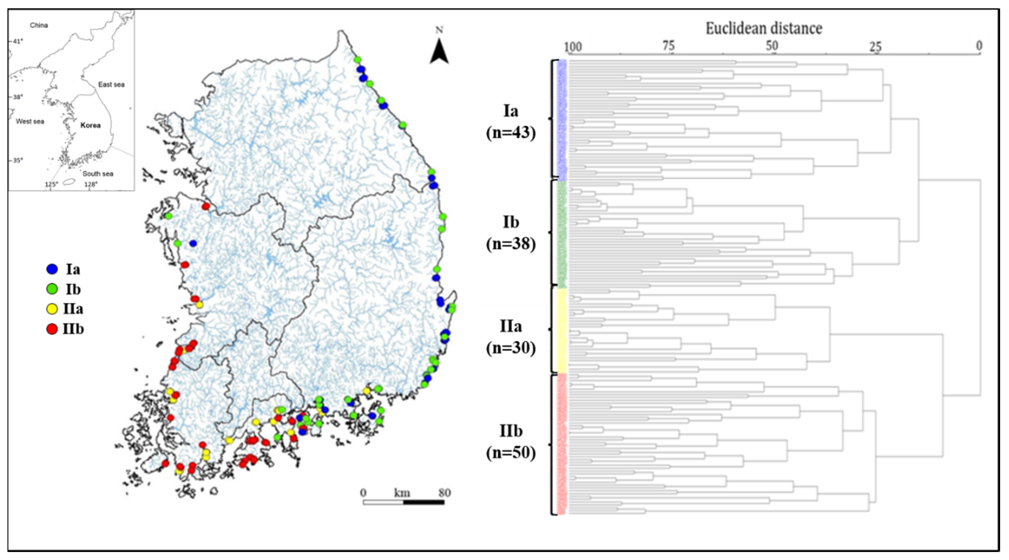
Map of 161 sampling sites for studies of water quality and epilithic diatoms in 90 Korean estuaries from 2012 to 2014; a: Dendrogram of site affinity based on diatom abundance, b: Colors in figures represent the same groups: Ia (blue), Ib (green), IIa (yellow), and IIb (red).
Figure 1.
Map of 161 sampling sites for studies of water quality and epilithic diatoms in 90 Korean estuaries from 2012 to 2014; a: Dendrogram of site affinity based on diatom abundance, b: Colors in figures represent the same groups: Ia (blue), Ib (green), IIa (yellow), and IIb (red).
2.2. Data Analysis
To understand the characteristics of diatom communities in the estuaries of the Korean peninsula, we conducted cluster analyses (CA) including all occurring species. We calculated the spatial patterns of diatom distribution and grouped samples according to similarities in the composition of diatom species using the Ward linkage method with Euclidean distance measures [53]. To observe the ecological characteristics of each community, the dominant index [54], diversity index [55], species richness index [56], and evenness index [57] were calculated per group. We also conducted an analysis of indicator species representative of each group using the indicator species analysis (ISA) method [58], which is a non-hierarchical statistical method. We calculated the indicator value (IndVal) using the relative richness and relative frequency of species occurring at each study site. In this study, a species in a group with an IndVal of more than 25 or with an IndVal greater than five times the IndVal of species in other groups was defined as a good indicator species for that group [59]. Among the diatom data used in CA and ISA, rare samples occurring at <5% of all total sites were excluded in the multivariate analysis. The remaining data were transformed by natural logarithms to reduce variation after adding one to all data to avoid the problem of an undefined logarithm zero. The analysis was performed using the PC-ORD software program (MjM Software, Gleneden Beach, OR, USA [60].
To understand the influences of environmental factors at each site on the distribution of diatoms, we conducted canonical correspondence analysis (CCA) [61]. CCA can be used to define composite environmental variables that correspond as closely as possible to the major patterns of species occurrence. CCA provides a direct gradient analysis of all species simultaneously in relation to the underlying gradients within the measured environmental variables [62,63]. Axes are derived that are linear combinations of environmental variables. Individual species are related directly to these axes under the assumption of a unimodal species response to the environmental variables. Canonical correspondence analysis is a means not only of directly investigating relationships between modern diatom assemblages and associated environmental variables but also indirectly of implementing weighted average calibration. The main advantages of weighted averaging ordinations include the simultaneous ordering of sites and species, rapid computation and very good performance when species have nonlinear and unimodal relationships to environmental gradients [64]. Meanwhile, a random forest (RF) model, a non-parametric method designed to predict and evaluate the relationship between potential predictor variables and dependent variables [65], was conducted to identify important environmental factors contributing to the occurrence of each diatom community. To compare the relative significance of each environmental factor, we used the minimum description length (MDL) [66]. To assess the predictability of the model, accuracy rates and the area under the curve (AUC) were calculated. The accuracy rates ranged from 0 to 1, and the AUC values ranged between 0.5 and 1 [67]. Canonical correspondence analysis was conducted using PC-ORD software [60], and the RF model was run using the CORElearn package in the R statistical program [68]. Analysis of variance (ANOVA) was carried out to compare the differences in environmental and biological characteristics among groups defined by correspondence analysis (CA). Tukey’s multiple comparison tests were used for post hoc comparisons. Pearson’s correlation analysis was performed to determine the relationship between the indicator species of each group and environmental factors. These analyses were conducted using SPSS software version 21 (IBM, New York, NY, USA).
3. Results
3.1. Characteristics of Epilithic Diatom Communities
A total of 327 diatom taxa with 10 families were recorded at 161 estuary sites in the Korean peninsula during the research period. Nitzschia inconspicua (17.1%) was the most abundant species in the estuaries of Korea, followed by Nitzschia frustulum (9.1%) and Nitzschia fonticola (7.3%). Among the five watershed areas, the Nakdong River area displayed the highest species richness with 207 species, whereas the East Han River area showed the lowest species richness with 140 species.
The diatom communities (except for rare species occurring in less than 5% of sites) in the 161 study sites were classified into two groups (I and II), with four subgroups based on their similarities by cluster analysis as follows: Ia (43 sites), Ib (38 sites), IIa (30 sites), and IIb (50 sites) (Figure 1). The site distribution in each group reflects the characteristics of the geographical locations of the sites. Most sites in Group I were situated in the East Sea and the eastern part of the South Sea, whereas the sites in Group II were located in the West Sea and the western part of the South Sea.
Community indices, except for biomass and the Shannon diversity index (H’), were significantly different among the four subgroups defined by cluster analysis (ANOVA, p < 0.05) (Table 1). The number of species and the richness index (R) showed higher values in Group I (Ia: 2.18 ± 0.09, Ib: 2.11 ± 0.16) (Tukey’s test, p < 0.05). Group IIb showed high values for the evenness index (E) (0.73 ± 0.02) but showed the lowest values for the dominance index (DI) (0.05 ± 0.02) (Tukey’s test, p < 0.05). Group IIa had the highest values for biomass (705.6 ± 178.1 × 10³ cells/cm2), although the biomass of Group IIa was not significantly different from the biomass of other clusters (Tukey’s test, p > 0.05).

Table 1.
Biological characteristics of Korean estuaries between 2012 and 2014. The estuaries were divided into four groups by cluster analysis based on diatom abundance. Small letters (a, b, and c) indicate Tukey’s test values. The P value is computed from the F ratio which is computed from the ANOVA table.
| Variables | Groups | F ratio | P value | |||
|---|---|---|---|---|---|---|
| Ia | Ib | IIa | IIb | |||
| Biomass (103 cells /cm2) | 566.4 ± 70.3 | 500.5 ± 67.2 | 705.6 ± 178.1 | 505.4 ± 69.7 | 0.878 | 0.454 |
| Number of species (No. /cm2) | 31.23 ± 1.36 b | 30.76 ± 2.20 b | 24.27 ± 1.40 a | 20.56 ± 0.87 a | 13.572 | <0.001 |
| Dominance index (DI) | 0.58 ± 0.21 ab | 0.57 ± 0.03 ab | 0.63 ± 0.03 b | 0.50 ± 0.02 a | 4.543 | 0.004 |
| Diversity index (H’) | 2.06 ± 0.08 | 2.07 ± 0.10 | 1.84 ± 0.09 | 2.11 ± 0.07 | 1.708 | 0.168 |
| Richness (R) | 2.18 ± 0.09 b | 2.11 ± 0.16 b | 1.45 ± 0.11 a | 1.37 ± 0.06 a | 16.966 | <0.001 |
| Evenness (E) | 0.61 ± 0.02 a | 0.63 ± 0.02 a | 0.64 ± 0.03 a | 0.73 ± 0.02 b | 7.460 | <0.001 |
Meanwhile, the family Naviculaceae had the highest occurrence (>40%) among the 10 diatom families, followed by the Bacillariaceae, Fragilariaceae, and Achnanthaceae families, all of which showed similar rates. Although such patterns did not vary by group, families Hemidiscaceae (Group Ia) and Entomoneidaceae (Group Ib) occurred in specific groups only (Table 2). Compared with the family Naviculaceae, which was the most diverse in terms of species, family Bacillariaceae (37.8%–61.7%) made up the majority of the diatom community, while families Naviculaceae, Fragilariaceae, Achnanthaceae, and Thalassiosiraceae accounted for relatively small proportions (Table 1). Such patterns varied by group. Families showing high abundance were Achnanthaceae (21.2%) in Group Ia, Naviculaceae (34.4%) in Group Ib, Bacillariaceae (61.7%) in Group IIa, and Thalassiosiraceae (6.2%) in Group IIb.
Table 2.
Species (N, %) and cell density (D, %) of epilithic diatom communities distributed in Korean estuaries between 2012 and 2014 at the family level. The estuaries were divided into four groups by cluster analysis based on diatom abundance.
| Family | Groups | |||||||
|---|---|---|---|---|---|---|---|---|
| Ia | Ib | IIa | IIb | |||||
| N | D | N | D | N | D | N | D | |
| Achnanthaceae | 12.26 | 21.22 | 11.70 | 2.97 | 12.50 | 3.34 | 10.49 | 10.69 |
| Bacillariaceae | 13.55 | 37.78 | 19.15 | 57.78 | 13.28 | 61.74 | 14.20 | 42.76 |
| Entomoneidaceae | 0.00 | 0.00 | 1.06 | 0.22 | 1.56 | 0.01 | 0.00 | 0.00 |
| Eunotiaceae | 1.29 | 0.04 | 1.06 | 0.01 | 0.78 | 0.00 | 1.23 | 0.14 |
| Fragilariaceae | 18.06 | 12.28 | 11.17 | 9.37 | 10.16 | 3.49 | 14.81 | 2.69 |
| Hemidiscaceae | 0.65 | 0.03 | 0.00 | 0.00 | 0.00 | 0.00 | 0.00 | 0.00 |
| Melosiraceae | 1.29 | 1.21 | 2.13 | 2.46 | 1.56 | 0.62 | 1.23 | 2.73 |
| Naviculaceae | 46.45 | 27.15 | 47.34 | 25.02 | 43.75 | 26.29 | 47.53 | 34.44 |
| Surirellaceae | 1.94 | 0.07 | 1.60 | 0.10 | 4.69 | 0.06 | 1.85 | 0.37 |
| Thalassiosiraceae | 4.52 | 0.22 | 4.79 | 2.08 | 11.72 | 4.45 | 8.64 | 6.18 |
| Real N&D | 155 | 2.4 × 10⁷ | 188 | 1.8 × 10⁷ | 128 | 2.1 × 10⁷ | 162 | 2.5 × 10⁷ |
3.2. Differences in Environmental Factors
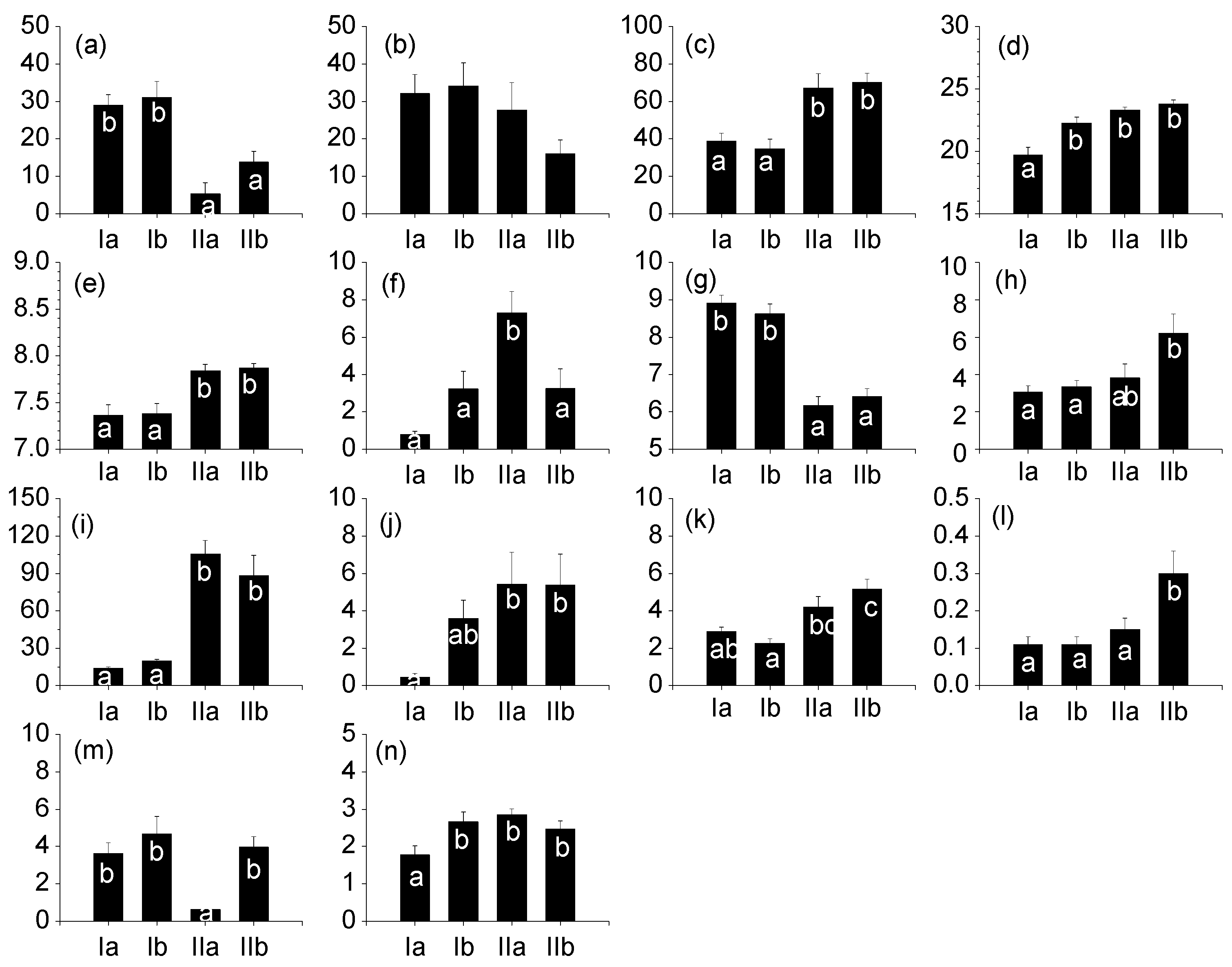
All environmental factors, except for urban area, were significantly different among groups (ANOVA, p < 0.05) (Figure 2). Group I (Ia and Ib) showed higher proportions of forest area than Group II (IIa and IIb) (Tukey’s test, p < 0.05), whereas the proportion of agricultural area was significantly higher in Group II (IIa and IIb) than in Group I (Ia and Ib) (Tukey’s test, p < 0.05). Water temperature was the lowest in Group Ia (19.70 ± 0.64 ° C) (Tukey’s test, p < 0.05). Dissolved oxygen (DO) values were found to be high in Groups Ia (8.91 ± 0.22 mg/L) and Ib (8.62 ± 0.27 mg/L), and the values of pH, BOD, electrical conductivity, TN, and TP were significantly higher in Group II (IIa and IIb) (Tukey’s test, p < 0.05) than in Group I. In particular, both turbidity (105.87 ± 10.54 NTU) and salinity (7.30 ± 1.15 ‰) were the highest in Group IIa (Tukey’s test, p < 0.05). Ash-free dry matter (AFDM) was the lowest in Group Ia (1.78 ± 0.23 mg/cm2), while chlorophyll-a (Chl-a) was the lowest in Group IIa (0.63 ± 0.05 μg/cm2) (Tukey’s test, p < 0.05).

Figure 2.
Environmental variables in four groups of Korean estuaries between 2012 and 2014. Small letters (a, b, and c) indicate Tukey’s post hoc test values. (a): forest area (%); (b): urban area (%); (c): argricultural area (%); (d): water temperature (°C); (e): pH; (f): salinity (permille); (g): DO (dissolved oxygen; mg/L); (h): BOD (biochemical oxygen demand; mg/L); (i): turbidity (NTU); (j): Electric conductivity (1000 μS/cm); (k): total nitrogen (mg/L); (l): total phosphorus (mg/L); (m): chlorophyll-a (mg/cm2); (n): AFDM(mg/cm2).
3.3. Correlations between Diatom Communities and Environment
To clarify the indicator species of each group, we carried out indicator species analysis on 136 taxa that occurred at more than 5% of all sites. Good indicator species with higher indicator values (IndVal) of 25% were identified in a total of 28 taxa, comprising Group Ia (11 species), Group Ib (4 species), Group IIa (10 species), and Group IIb (three species). The highest good indicator species (IndVal > 50%) were Navicula saprophila (67%) and Reimeria sinuata (51%) in Group Ia and Encyonema minutum (60%) in Group IIa. On the other hand, all the indicator species showed low IndVal (<40%) in Group Ib and Group IIb (Table 3). Overall, the indicator species showed high correlations with turbidity and electrical conductivity(EC). Negative correlations were observed in Groups Ia and Ib (with the exception of EC), but positive correlations were observed in Groups IIa and IIb (Table 3). The indicator species in Group Ia (Navicula saprophila, Reimeria sinuata, Gomphonema pseudoaugur, and Fragilaria capucina var. gracilis) showed positive correlations with the proportion of forest area and dissolved oxygen (DO), but negative correlations with water temperature, pH, salinity, turbidity, electrical conductivity (EC), and AFDM. Rhoicosphenia abbreviata, the indicator species in Group Ib, showed positive correlations with the proportion of forest area and values of dissolved oxygen (DO) and chlorophyll-a (chl-a), but negative correlations with turbidity and electrical conductivity (EC). The remaining indicator species showed strongly negative correlations with turbidity.
Table 3.
Correlation coefficients among indicator species and environmental variables in each group of Korean estuaries between 2012 and 2014.
| CODE | Forest | Urban | AGR | WT | pH | SAL | DO | BOD | TURB | EC | TN | TP | N/P | Chl-a | AFDM | Group |
|---|---|---|---|---|---|---|---|---|---|---|---|---|---|---|---|---|
| NASP | 0.27 ** | 0.18 * | −0.12 | −0.53 ** | −0.35 ** | −0.17 * | 0.44 ** | −0.11 | −0.45 ** | −0.35 ** | −0.11 | −0.15 | 0.15 | 0.06 | −0.34 ** | Ia |
| RESI | 0.33 ** | 0.07 | −0.06 | −0.34 ** | −0.19 * | −0.24 ** | 0.29 ** | −0.31 ** | −0.46 ** | −0.42 ** | −0.18 * | −0.25 ** | 0.20 * | 0.04 | −0.28 * | Ia |
| GOPS | 0.20 * | 0.21 ** | −0.16 * | −0.40 ** | −0.22 ** | −0.21 ** | 0.40 ** | −0.08 | −0.35 ** | −0.33 ** | −0.06 | −0.07 | 0.06 | 0.18 * | −0.22 ** | Ia |
| FRVG | 0.20 * | 0.18 * | −0.03 | −0.40 ** | −0.09 | −0.21 ** | 0.26 ** | −0.11 | −0.32 ** | −0.37 ** | −0.01 | −0.08 | 0.16 * | 0.12 | −0.28 ** | Ia |
| COVL | 0.18 * | 0.26 ** | −0.24 ** | −0.27 ** | −0.15 | −0.17 * | 0.19 * | −0.08 | −0.24 ** | −0.27 ** | 0.00 | −0.06 | 0.01 | 0.11 | −0.13 | Ia |
| NAMN | 0.14 | 0.17 * | −0.05 | −0.25 ** | −0.08 | −0.15 | 0.15 * | −0.16 * | −0.26 ** | −0.25 ** | 0.01 | −0.08 | 0.12 | 0.07 | −0.30 ** | Ia |
| NASU | 0.18 * | 0.19 * | −0.06 | −0.46 ** | −0.08 | −0.15 | 0.24 ** | −0.04 | −0.27 ** | −0.29 ** | 0.00 | −0.05 | 0.09 | 0.09 | −0.27 ** | Ia |
| FRRV | 0.13 | 0.24 ** | −0.21 ** | −0.40 ** | −0.13 | −0.13 | 0.27 ** | −0.14 | −0.27 ** | −0.27 ** | −0.09 | −0.13 | 0.11 | −0.01 | −0.32 ** | Ia |
| NASM | 0.14 | 0.18 * | −0.13 | −0.52 ** | 0.02 | −0.02 | 0.14 | −0.07 | −0.23 ** | −0.15 | 0.07 | −0.17 * | 0.26 ** | 0.02 | −0.35 ** | Ia |
| FRRU | 0.12 | 0.24 ** | −0.13 | −0.47 ** | −0.15 | −0.06 | 0.34 ** | −0.01 | −0.29 ** | −0.20 * | −0.08 | −0.18 * | 0.22 ** | −0.01 | −0.28 ** | Ia |
| ACSU | 0.14 | 0.03 | 0.00 | −0.29 ** | −0.12 | −0.12 | 0.23 ** | −0.03 | −0.26 ** | −0.26 ** | −0.03 | −0.13 | 0.14 | 0.07 | −0.25 ** | Ia |
| RHAB | 0.25 ** | 0.08 | −0.14 | −0.04 | −0.13 | −0.02 | 0.33 ** | 0.00 | −0.31 ** | −0.03 | −0.14 | −0.14 | −0.04 | 0.31 ** | 0.07 | Ib |
| FRFA | 0.14 | 0.20 * | −0.23 ** | −0.07 | −0.09 | 0.14 | 0.13 | 0.03 | −0.14 | 0.21 ** | −0.17 * | −0.15 | 0.02 | 0.06 | 0.07 | Ib |
| DESU | 0.05 | 0.13 | −0.23 ** | −0.04 | −0.12 | 0.19 * | 0.14 | −0.01 | −0.05 | 0.12 | −0.11 | −0.09 | −0.02 | 0.01 | −0.05 | Ib |
| NAIN | 0.10 | 0.15 | −0.19 * | 0.13 | −0.03 | 0.12 | 0.10 | −0.07 | −0.07 | 0.15 | −0.12 | −0.03 | −0.07 | 0.10 | 0.13 | Ib |
| ENMI | −0.32 ** | −0.04 | −0.01 | 0.12 | 0.16 * | 0.32 ** | −0.20 ** | −0.07 | 0.33 ** | 0.14 | 0.10 | −0.02 | 0.19 * | −0.31 ** | 0.16 * | IIa |
| RHCU | −0.15 | −0.09 | 0.09 | 0.10 | 0.11 | 0.23 ** | −0.20 * | −0.10 | 0.32 ** | 0.21 ** | 0.04 | −0.08 | 0.19 * | −0.30 ** | 0.17 * | IIa |
| TAFA | −0.30 ** | −0.02 | 0.00 | 0.09 | 0.14 | 0.25 ** | −0.30 ** | −0.01 | 0.31 ** | 0.11 | 0.00 | −0.01 | 0.02 | −0.25 ** | 0.10 | IIa |
| AMHO | −0.20 ** | −0.12 | 0.11 | 0.10 | −0.01 | 0.37 ** | −0.13 | −0.07 | 0.22 ** | 0.26 ** | 0.01 | −0.09 | 0.12 | −0.31 ** | 0.01 | IIa |
| ACLO | −0.23 ** | −0.02 | 0.07 | 0.09 | 0.09 | 0.31 ** | −0.20 * | 0.00 | 0.26 ** | 0.21 ** | 0.04 | −0.03 | 0.06 | −0.26 ** | 0.07 | IIa |
| NACN | −0.24 ** | −0.07 | 0.09 | 0.14 | 0.12 | 0.27 ** | −0.18 * | −0.05 | 0.28 ** | 0.12 | 0.05 | 0.00 | 0.05 | −0.24 ** | 0.07 | IIa |
| NACP | −0.16 * | −0.09 | 0.15 | 0.14 | 0.13 | 0.30 ** | −0.29 ** | −0.02 | 0.37 ** | 0.24 ** | 0.12 | 0.15 | −0.07 | −0.13 | 0.05 | IIa |
| ACEX | −0.16 * | −0.06 | 0.14 | 0.14 | 0.13 | 0.02 | −0.21 ** | 0.22 ** | 0.29 ** | 0.11 | 0.10 | 0.10 | −0.03 | −0.05 | 0.01 | IIa |
| NAHI | −0.18 * | −0.06 | 0.06 | 0.11 | 0.15 | 0.28 ** | −0.16 * | −0.09 | 0.19 * | 0.10 | 0.14 | −0.01 | 0.17 * | −0.21 ** | 0.10 | IIa |
| CYAT | −0.22 ** | −0.05 | −0.02 | 0.15 | 0.11 | 0.31 ** | −0.09 | −0.17 * | 0.22 ** | 0.17 * | −0.11 | −0.11 | 0.07 | −0.20 * | 0.07 | IIa |
| CYME | −0.16 * | −0.10 | 0.13 | 0.14 | 0.17 * | −0.19 * | −0.13 | 0.26 ** | 0.24 ** | 0.01 | 0.12 | 0.15 | −0.09 | 0.12 | −0.03 | IIb |
| NASA | −0.18 * | −0.02 | 0.06 | 0.21 ** | 0.18 * | 0.09 | −0.12 | 0.30 ** | 0.30 ** | 0.25 ** | 0.25 ** | 0.23 ** | −0.14 | 0.13 | 0.06 | IIb |
| FRBI | −0.11 | −0.07 | 0.19 * | 0.01 | 0.17 * | −0.12 | −0.13 | 0.00 | 0.00 | 0.00 | 0.09 | −0.01 | 0.02 | 0.03 | −0.07 | IIb |
NASP: Navicula saprophila, RESI: Reimeria sinuata, GOPS: Gomphonema pseudoaugur, FRVG: Fragilaria capucina var. gracilis, COVL: Cocconeis placentula var. lineata, NAMN: Navicula minuscula, NASU: Navicula subatomoides, FRRV: Fragilaria rumpens var. fragilarioides, NASM: Navicula seminulum, FRRU: Fragilaria rumpens, ACSU: Achnanthes subhudsonis, RHAB: Rhoicosphenia abbreviata, FRFA: Fragilaria fasiculata, DESU: Denticula subtilis, NAIN: Navicula incerata, ENMI: Encyonema minutum, RHCU: Rhoicosphenia curvata, TAFA: Tabularia fasciculata, AMHO: Amphora holsatica, ACLO: Achnanthes longipes, NACN: Navicula canalis, NACP: Navicula capitatoradiata, ACEX: Achnanthes exigua, NAHI: Navicula hintzii, CYAT: Cyclotella atomus, CYME: Cyclotella meneghiniana, NASA: Navicula salinarum, FRBI: Fragilaria bidens. * p < 0.05, ** p < 0.01.
3.4. Environmental Effects on the Spatial Distribution of Diatoms
We performed CCA to determine the effects of environmental factors on the distribution of epilithic diatoms. The distribution of diatom communities is explained by the two ordination axes in CCA (eigenvalues: 0.308 in Axis-1 and 0.160 in Axis-2). Group Ia is located on the right side of Axis-1, and Group Ib is closer to the origin than Group Ia. Group IIa is positioned on the left side of Axis-1, and Group IIb is located on the bottom of Axis-2. The effects of environmental factors were identified by correlation coefficients (Pearson correlation coefficient, p < 0.05) between environmental factors and each axis. Correlation coefficients are shown as arrows on the CCA ordination (Figure 3c), where the arrow length indicates the magnitude of the correlation value and the arrow direction implies a correlation with each axis. Axis-1 was most highly correlated with turbidity (r = −0.816), followed by dissolved oxygen (r = 0.631), salinity (r = −0.579), proportion of forest area (r = 0.561), and electrical conductivity (r = −0.559). Axis-2 showed a high correlation with BOD (r = −0.535), chlorophyll-a (r = 0.382), salinity (r = 0.380), and total phosphorus (r = −0.364) (Figure 3d).
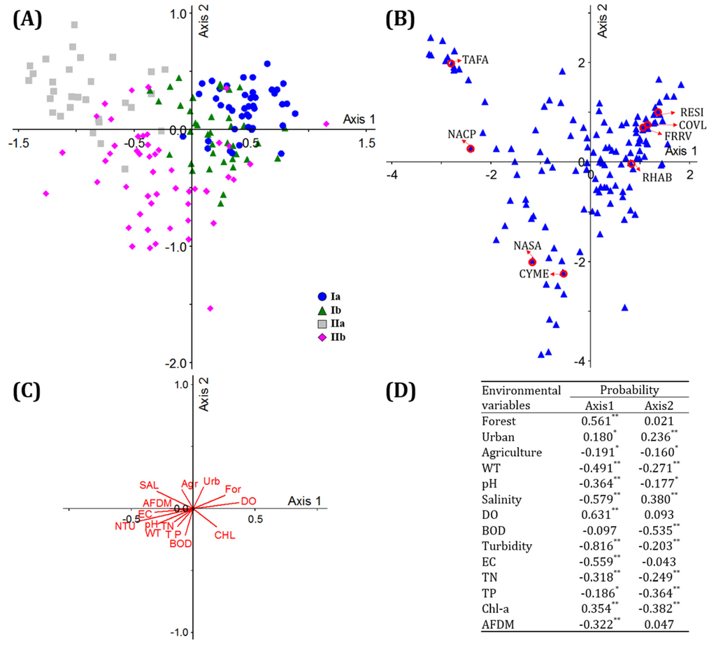
Figure 3.
(A) CCA ordination showing the distribution of four diatom groups in Korean estuaries between 2012 and 2014; (B) Distributions of epilithic diatoms, including indicator species; (C) Environmental variables affecting epilithic diatom distribution; (D) Correlation coefficients between environmental variables and CCA Axes-1 and 2. * p < 0.05, ** p < 0.01 For: forest, Urbe: urban, Agr: agriculture, WT: water temperature, SAL: salinity, DO: dissolved oxygen, BOD: biochemical oxygen demand, NTU: turbidity, EC: electric conductivity, TN: total nitrogen, TP: total phosphorus, chl-a: chlorophyll-a, AFDM: ash-free-dry-matter, NS: no. species, RESI: Reimeria sinuata, COVL: Cocconeis placentula var. lineata, FRRV: Fragilaria rumpens var. fragilarioides, RHAB: Rhoicosphenia abbreviata, TAFA: Tabularia fasciculata, NACP: Navicula capitatoradiata, CYME: Cyclotella meneghiniana, NASA: Navicula salinarum.

3.5. Predictions of the Appearance of Diatom Species
Appearances of species in diatom communities were predicted according to environmental factors using a random forest model. The performance measures were different depending on species, ranging from 0.76 to 0.95 in accuracy and from 0.94 and 1.00 in AUC (Table 4). Among the 136 taxa, four species (Amphora fontinalis, Cocconeis sp., Eunotia minor, Navicula bacillum) exhibited a relatively high predictive power (accuracy: 0.95, AUC: 1.00), whereas Navicula cryptotenella and Achnanthes brevipes showed relatively low accuracy regarding prediction (0.76 and 0.79, respectively). To evaluate the contribution of environmental factors in predicting the occurrence of each diatom species, sensitivity analysis was conducted using the minimum description length (MDL) in RF. The most important factors impacting the occurrence of epilithic diatoms were turbidity (35 species, 26%), electrical conductivity (28 species, 21%), and salinity (14 species, 10%). These factors explained the appearance of 57% of total species in all the diatom communities of each site. Concentrations of TN (12 species, 9%) and TP (11 species, 8%) were also shown to be of relatively high importance for species appearance in diatom communities (Table 4). Other important factors were electrical conductivity for Navicula saprophila and Reimeria sinuata, which are the indicator species of Group Ia with high indicator values (>60%), and turbidity for Encyonema minutum, which is the indicator species of Group IIa (Table 4).
Table 4.
List of epilithic diatoms with the first and second most important variables predicting species appearance by a random forest model in Korean estuaries between 2012 and 2014. Ar: accuracy rate, AUC: area under the curve, GI: group indicator.
| Species | Ar | AUC | Important Variables | GI | |
|---|---|---|---|---|---|
| 1st | 2nd | ||||
| Achnanthes alteragracillima Lange-Bertalot | 0.93 | 0.99 | pH | TURB | – |
| Achnanthes brevipes Agardh | 0.79 | 0.98 | EC | SAL | – |
| Achnanthes convergens Kobayasi, Nagumo & Mayama | 0.87 | 0.95 | TURB | EC | – |
| Achnanthes delicatula (Kützing) Grunow | 0.81 | 0.98 | Forest | TURB | – |
| Achnanthes exigua Grunow | 0.84 | 0.95 | TURB | BOD | IIa |
| Achnanthes lanceolata (Brébisson) Grunow | 0.87 | 0.94 | Forest | TURB | – |
| Achnanthes laterostrata Hustedt | 0.90 | 0.98 | TP | TURB | – |
| Achnanthes longipes Agardh | 0.94 | 1.00 | Urban | SAL | IIa |
| Achnanthes minutissima Kützing | 0.93 | 0.98 | EC | TP | – |
| Achnanthes subhudsonis Hustedt | 0.91 | 0.99 | pH | SAL | Ia |
| Amphora coffeaeformis (Agardh)Kützing | 0.91 | 0.99 | SAL | pH | – |
| Amphora copulate (Kützing) Schoeman and Archibald | 0.90 | 1.00 | TP | EC | – |
| Amphora fontinalis Hustedt | 0.95 | 1.00 | AGR | Urban | – |
| Amphora holsatica Hustedt | 0.93 | 0.97 | SAL | AGR | IIa |
| Amphora pediculus (Kützing) Grunow in Van Heurck | 0.91 | 0.99 | TN | SAL | – |
| Amphora sp. | 0.91 | 0.98 | SAL | DO | – |
| Amphora veneta Kützing | 0.93 | 1.00 | EC | Forest | – |
| Aulacoseira alpigena (Grunow) Krammer | 0.92 | 0.98 | Forest | SAL | – |
| Aulacoseira ambigua (Grunow) Simonsen | 0.91 | 0.99 | TP | Urban | – |
| Aulacoseira granulata (Ehrenberg) Simonsen | 0.93 | 0.99 | DO | SAL | – |
| Bacillaria paradoxa Gmelin | 0.88 | 1.00 | EC | SAL | – |
| Cocconeis placentula Ehrenberg | 0.85 | 0.96 | TURB | TP | – |
| Cocconeis placentula var. euglypta (Ehrenberg) Grunow | 0.92 | 0.99 | EC | TN | – |
| Cocconeis placentula var. lineata (Ehrenberg) Van Heurck | 0.87 | 0.98 | EC | SAL | Ia |
| Cocconeis sp. | 0.95 | 1.00 | TURB | SAL | – |
| Cyclotella atomus Hustedt | 0.91 | 0.98 | TURB | BOD | IIa |
| Cyclotella meneghiniana Kützing | 0.86 | 0.96 | SAL | EC | IIb |
| Cyclotella pseudostelligera Hustedt | 0.86 | 0.99 | EC | DO | – |
| Cyclotella stelligera Cleve & Grunow | 0.95 | 0.99 | TURB | SAL | – |
| Cymbella affinis Kützing | 0.83 | 0.99 | TURB | BOD | – |
| Cymbella minuta Hilse in Rabenhorst | 0.80 | 0.95 | EC | SAL | – |
| Cymbella silesiaca Bleisch in Rabenhorst | 0.94 | 0.98 | TURB | DO | – |
| Denticula subtilis Grunow | 0.93 | 0.99 | SAL | DO | Ib |
| Diatoma vulgaris Bory | 0.93 | 1.00 | TURB | EC | – |
| Diploneis oblongella (Nägeli) Cleve-Euler | 0.94 | 1.00 | EC | TURB | – |
| Diploneis subovalis Cleve | 0.90 | 0.98 | TURB | EC | – |
| Encyonema minutum (Hilse) Mann | 0.91 | 0.99 | TURB | TP | IIa |
| Entomoneis alata (Ehrenberg) Ehrenberg | 0.95 | 0.99 | EC | SAL | – |
| Eunotia minor (Kützing) Grunow | 0.95 | 1.00 | BOD | TP | – |
| Fragilaria bidens Heiberg | 0.92 | 1.00 | TURB | BOD | IIb |
| Fragilaria capitellata (Grunow) J.B.Petersen | 0.89 | 0.97 | AGR | TP | – |
| Fragilaria capucina Desmazières | 0.83 | 0.97 | TP | EC | – |
| Fragilaria capucina var. gracilis (Østrup) Hustedt | 0.91 | 0.95 | EC | Urban | Ia |
| Fragilaria capucina var. radians (Kützing) Lange-Bertalot | 0.94 | 0.99 | TP | AGR | – |
| Fragilaria construens f. venter (Ehrenberg) Hustedt | 0.95 | 0.99 | TURB | pH | – |
| Fragilaria delicatissima (W. Smith) Lange-Bertalot | 0.94 | 0.97 | DO | AGR | – |
| Fragilaria elliptica Schumann | 0.84 | 0.96 | TURB | TN | – |
| Fragilaria fasiculata (Agardh) Lange-Bertalot | 0.89 | 0.98 | TURB | EC | Ib |
| Fragilaria pinnata Ehrenberg | 0.87 | 0.98 | pH | BOD | – |
| Fragilaria rumpens (Kützing) G.W.F. Carlson | 0.90 | 0.98 | AGR | EC | Ia |
| Fragilaria rumpens var. familiaris (Kützing) Cleve-Euler | 0.88 | 0.97 | pH | Urban | – |
| Fragilaria rumpens var. fragilarioides (Grunow) Cleve-Euler | 0.89 | 0.97 | EC | Urban | Ia |
| Fragilaria sp. | 0.94 | 0.99 | TURB | SAL | – |
| Fragilaria vaucheriae (Kützing) Petersen | 0.92 | 0.98 | EC | BOD | – |
| Gomphonema angustatum (Kützing) Rabenhorst | 0.93 | 0.98 | TN | SAL | – |
| Gomphonema angustum Agardh | 0.95 | 0.99 | EC | Urban | – |
| Gomphonema clevei Fricke in Schmidt | 0.88 | 0.97 | TN | TURB | – |
| Gomphonema lagenula Kützing | 0.81 | 0.96 | SAL | BOD | – |
| Gomphonema minutum (Agardh) Agardh | 0.90 | 1.00 | Urban | AGR | – |
| Gomphonema parvulum (Kützing) Kützing | 0.83 | 1.00 | TURB | TN | – |
| Gomphonema pseudoaugur Lange-Bertalot | 0.92 | 0.97 | TURB | DO | Ia |
| Gomphonema quadripunctatum (Østrup) Wislouch | 0.94 | 0.99 | AGR | Forest | – |
| Gomphonema sp. | 0.91 | 0.98 | EC | pH | – |
| Gyrosigma acuminatum (Kützing) Rabenhorst | 0.91 | 1.00 | TURB | AGR | – |
| Melosira nummuloides Agardh | 0.94 | 1.00 | TN | TURB | – |
| Melosira varians Agardh | 0.90 | 0.98 | BOD | TURB | – |
| Meridion circulare var. constrictum (Ralfs) Van Heurck | 0.93 | 0.98 | TURB | AGR | – |
| Navicula accomoda Hustedt | 0.89 | 0.99 | Forest | SAL | – |
| Navicula atomus (Kützing) Grunow | 0.93 | 1.00 | TN | BOD | – |
| Navicula bacillum Ehrenberg | 0.95 | 1.00 | TP | EC | – |
| Navicula canalis Patrick | 0.94 | 0.99 | SAL | EC | IIa |
| Navicula capitata Ehrenberg | 0.90 | 0.98 | TURB | pH | – |
| Navicula capitatoradiata Germain | 0.93 | 0.99 | TURB | SAL | IIa |
| Navicula cari Ehrengerg | 0.93 | 0.99 | TURB | pH | – |
| Navicula cincta (Ehrengerg) Ralfs in Pritchard | 0.86 | 0.99 | TURB | BOD | – |
| Navicula cryptocephala Kützing | 0.86 | 0.98 | EC | DO | – |
| Navicula cryptotenella Lange-Bertalot | 0.76 | 0.98 | AGR | EC | – |
| Navicula decussis Østrup | 0.89 | 0.97 | TN | AGR | – |
| Navicula goeppertiana (Bleisch in Rabenhorst) H. L. Smith | 0.93 | 0.99 | Urban | Forest | – |
| Navicula gregaria Donkin | 0.90 | 0.98 | pH | TURB | – |
| Navicula hintzii Lange-Bertalot | 0.95 | 0.99 | EC | TP | IIa |
| Navicula incerta Grunow in Van Heurck | 0.93 | 1.00 | EC | SAL | Ib |
| Navicula menisculus Schumann | 0.94 | 1.00 | TURB | BOD | – |
| Navicula minima Grunow in Van Heurck | 0.90 | 0.97 | Urban | EC | – |
| Navicula minuscula Grunow in Van Heurck | 0.87 | 0.96 | EC | TP | Ia |
| Navicula mutica Kützing | 0.94 | 0.99 | SAL | EC | – |
| Navicula mutica var. ventricosa (Kützing) Cleve & Grunow | 0.94 | 0.99 | TURB | DO | – |
| Navicula perminuta (Kützing) Cleve & Grunow | 0.89 | 0.96 | DO | TURB | – |
| Navicula pupula Kützing | 0.84 | 0.97 | TN | TP | – |
| Navicula radiosa Kützing | 0.91 | 1.00 | BOD | TP | – |
| Navicula recens (Lange-Bertalot) Lange-Bertalot | 0.88 | 0.96 | TURB | TP | – |
| Navicula rhynchocephala Kützing | 0.88 | 0.98 | DO | Urban | – |
| Navicula salinarum Grunow in Cleve & Grunow | 0.89 | 0.97 | EC | TN | IIb |
| Navicula saprophila Lange-Bertalot & Bonik | 0.93 | 0.98 | EC | pH | Ia |
| Navicula schroeteri Meister | 0.88 | 0.99 | TURB | SAL | – |
| Navicula seminuloides Hustedt | 0.94 | 0.99 | TP | pH | – |
| Navicula seminulum Grunow | 0.89 | 0.96 | EC | TN | Ia |
| Navicula sp. | 0.94 | 0.99 | SAL | TURB | – |
| Navicula stroemii Hustedt | 0.93 | 0.98 | TP | pH | – |
| Navicula subatomoides Hustedt | 0.91 | 0.99 | TN | EC | Ia |
| Navicula subminuscula Manguin | 0.86 | 0.95 | DO | EC | – |
| Navicula tripunctata (O.F. Müller) Bory | 0.84 | 0.95 | SAL | EC | – |
| Navicula trivialis Lange-Bertalot | 0.88 | 0.96 | DO | SAL | – |
| Navicula veneta Kützing | 0.83 | 0.99 | DO | EC | – |
| Navicula viridula (Kützing) Ehrenberg | 0.93 | 0.99 | TP | DO | – |
| Navicula viridula var. rostellata (Kützing) Cleve | 0.86 | 0.98 | EC | TURB | – |
| Nitzschia amphibian Grunow | 0.89 | 0.96 | DO | BOD | – |
| Nitzschia calida Grunow in Cleve & Grunow | 0.93 | 0.99 | DO | SAL | – |
| Nitzschia capitellata Hustedt | 0.91 | 0.99 | pH | Urban | – |
| Nitzschia communis Rabenhorst | 0.93 | 0.99 | DO | pH | – |
| Nitzschia constricta (Kützing) Ralfs | 0.92 | 0.99 | SAL | TN | – |
| Nitzschia dissipata (Kützing) Grunow | 0.84 | 0.99 | AGR | EC | – |
| Nitzschia filiformis (W. Smith) Hustedt | 0.89 | 0.97 | AGR | TP | – |
| Nitzschia fonticola Grunow in Cleve & Möller | 0.88 | 0.97 | TURB | DO | – |
| Nitzschia frustulum (Kützing) Grunow in Cleve & Grunow | 0.93 | 0.98 | SAL | pH | – |
| Nitzschia gracilis Hantzsch | 0.85 | 0.96 | TN | BOD | – |
| Nitzschia inconspicua Grunow | 0.83 | 0.97 | EC | SAL | – |
| Nitzschia littoralis Grunow in Cleve & Grunow | 0.94 | 0.99 | SAL | BOD | – |
| Nitzschia palea (Kützing) W. Smith | 0.87 | 0.97 | AGR | EC | – |
| Nitzschia paleacea (Grunow) Grunow in Van Heurck | 0.92 | 0.99 | DO | TP | – |
| Nitzschia pellucida Grunow | 0.95 | 0.99 | TN | TURB | – |
| Nitzschia perminuta (Grunow) M. Peragallo | 0.93 | 0.99 | TURB | DO | – |
| Nitzschia recta Hantzsch in Rabenhorst | 0.94 | 1.00 | pH | TURB | – |
| Nitzschia sp. | 0.93 | 1.00 | TURB | SAL | – |
| Nitzschia subacicularis Hustedt in A. Schmidt et al. | 0.95 | 0.99 | EC | SAL | – |
| Nitzschia tryblionella Hantzsch in Rabenhorst | 0.93 | 1.00 | TP | TN | – |
| Reimeria sinuata (Gregory) Kociolek & Stoermer | 0.93 | 0.97 | EC | TURB | Ia |
| Rhoicosphenia abbreviata (Agardh) Lange-Bertalot | 0.91 | 0.98 | TURB | DO | Ib |
| Rhoicosphenia curvata (Kützing) Grunow | 0.91 | 0.99 | TURB | SAL | IIa |
| Surirella angusta Kützing | 0.93 | 0.98 | SAL | TURB | – |
| Surirella minuta Brébisson in Kützing | 0.87 | 0.98 | pH | Forest | – |
| Surirella ovalis Brébisson | 0.94 | 1.00 | TN | EC | – |
| Synedra acus Kützing | 0.93 | 0.99 | TN | TURB | – |
| Synedra pulchella (Ralfs in Kützing) Kützing | 0.94 | 0.99 | TURB | pH | – |
| Synedra ulna (Nitzsch) Ehrenberg | 0.81 | 0.98 | TP | TURB | – |
| Tabularia fasciculata (Agardh) Williams & Round | 0.91 | 0.99 | TURB | EC | IIa |
4. Discussion
The present study analyzes the distribution and abundance of diatom communities in estuaries of the Korean peninsula in relation to environmental conditions. A total of 327 diatom taxa were recorded at 161 sites in estuaries in the Korean peninsula during the research period. In comparison to previous studies identifying 284 taxa in 58 sites in 2012 [69] and 171 taxa in 38 sites in 2013 [2], our sample is more diverse, likely because the present study includes more sites than previous studies. With regard to the occurrence of diatom species in each group, Group Ib includes the largest number of diatom taxa (188 species), while Group IIa includes the smallest number of diatom taxa (128 species). In contrast, the abundance of diatoms was highest in Group IIb (2.5 × 10⁷ cells/cm2) and was lowest in Group Ib (1.8 × 10⁷ cells/cm2). However, there were no significant differences among groups (ANOVA, p > 0.05).
The overall sample of diatom communities in the estuaries of the Korean peninsula was classified into four subgroups through cluster analysis based on similarities in community composition. These four subgroups were reclassified into two groups, groups I and II, reflecting the characteristics of the geographical locations of the sites. The diatom communities comprising Group I were located near the East Sea and the eastern part of the South Sea, including the East Han River watershed and the Nakdong River watershed. The East Sea maintains high water quality due to its composition of land use/cover, which includes forest (more than 60%) and agricultural land use/cover (less than 20%) [3]. Group II is comprised of diatom communities from the West Sea and the western part of the South Sea, including the Geum River and Yeongsan River watersheds. The proportion of agricultural land use/cover is far higher (more than 35%) in Group II than the average proportion of agricultural land use/cover in the rest of South Korea (28.8%). In addition, large-scale reclamation projects and land development work have resulted in severe water pollution of the streams in the region [3]. In comparison to Group II, the regions of Group I have fewer nutrients with lower salinity and turbidity (ANOVA, p < 0.05; Figure 2). This finding coincides with the findings of previous studies, which assert that forest land cover has a negative correlation with nutrients [70,71]. In addition, streams in the east coastal area of Korea are characterized by a series of ridges with decreasing altitudes from the Taebaek Mountains to the East Sea. Thus, small streams flowing into the East Sea have steep bed slopes and short river channels [72]. The tidal effects are usually weak on the east coast of Korea due to this small tidal range [73]. Meanwhile, Group II has a relatively higher proportion of agricultural land use/cover, more nutrients, higher electrical conductivity, and higher turbidity (Figure 2). In general, high proportions of agricultural land use/cover lead to higher concentrations of zinc, lead, cadmium, and manganese, as well as higher concentrations of nutrients (total nitrogen and total phosphorus), which aggravates water pollution [71,74,75,76]. Furthermore, the west coastal area of Korea has always had high turbidity levels due to its relatively large tidal range [77].
Indicator species in each group were determined through IndVal analysis, and the impact of environmental conditions on the indicator species was indicated. Among them, Reimeria sinuata, Cocconeis placentula var. lineata and Fragilaria rumpens var. fragilarioides in Group Ia and Rhoicosphenia abbreviata in Group Ib were positively correlated with dissolved oxygen (DO) and the proportion of forest land use/cover (Table 3, Figure 3). These saproxenous taxa are generally found in oligotrophic-mesotrophic waters [78,79] with high levels of dissolved oxygen (DO), and all of them occur in oceans, brackish water, or freshwater zones with high electrical conductivity [80]. In addition, saprophilous taxa, such as Cyclotella meneghiniana and Navicula salinarum in Group IIb, have positive correlations with BOD, but a negative correlation with the proportion of forest land use/cover (Table 3). These taxa usually occur in polluted streams [81,82,83,84,85]. Tabularia fasciculata and Navicula capitatoradiata of Group IIa are positively correlated with salinity (Table 3). Previous studies [80,86] indicate that these are cosmopolitan species that favor saline brackish water zones or waters of high electrical conductivity.
A random forest model is a non-parametric method for predicting and assessing the relationships between a large number of potential predictor variables and repose variables [87]. Through demonstration of their high capability for modeling ecological problems involving non-linear relationships between data, random forest models are known to have learning and predicative power, as well as explanatory capacity [88]. In this study, we predict the occurrence of epilithic diatom communities using a random forest model based on differences in environmental factors. The importance of environmental factors used in the RF model was evaluated using the minimum description length (MDL), which measures the quality of attributes according to their ability to compress the data [66]. According to our evaluation of the relative importance of environmental factors for the prediction of epilithic diatom communities, the factors that exhibited relatively higher importance in their contributions were physicochemical factors (over other factors such as land use/cover) based on the MDL in the RF model (Table 4). The most important factors affecting the occurrence of epilithic diatoms were turbidity (35 species, 26%), electrical conductivity (28 species, 21%), and salinity (14 species, 10%). These factors explained the appearance of 57% of total species in all the diatom communities of each site. The concentrations of TN (12 species, 9%) and TP (11 species, 8%) also showed relatively high importance (Table 4). Turbidity refers to reduced amounts of DO through the blocking of light, which is required in the short run for photosynthesis. In the long run, turbidity induces the growth of algae in water by gradually dissolving particulate nutrients that flow in with silt [89,90]. In addition, electrical conductivity plays an important role in driving the structure and composition of diatom communities in the estuaries of the Korean peninsula [91,92].
Acknowledgments
This study was supported by the Ministry of Environment and the National Institute of Environmental Research (Korea). The authors would like to thank all of the survey members involved in the project for their help in sampling and analyses. The authors also thank the reviewers for their help in improving the scientific quality of the manuscript.
Author Contributions
Ha-Kyung Kim, Yong-Jae Kim, and Baik-Ho Kim collected the diatom samples. Baik-Ho Kim contributed to the writing of the manuscript and participated in discussions regarding the appropriate groups for analysis, and Yong-Su Kwon helped in manuscript revision. All the authors approved the final manuscript.
Conflicts of Interest
The authors declare no conflict of interest.
References
- Harrison, J.D.; Cooper, J.A.G.; Ramm, A.E.L. State of South African Estuaries: Geomorphology Ichthyofauna, Water Quality and Aesthetics; Department of Environmental Affairs and Tourism: Pretoria, South Africa, 2000.
- Kim, H.K.; Lee, M.H.; Kim, Y.J.; Won, D.H.; Hwang, S.J.; Hwang, S.O.; Kim, S.H.; Kim, B.H. Water Quality and Epilithic Diatom Community in the Lower Stream near the South Harbor System of Korean Peninsula. Korean J. Ecol. Environ. 2013, 46, 551–560. [Google Scholar]
- Rho, P.H.; Lee, C.H. Spatial Distribution and Temporal Variation of Estuarine Wetlands by Estuary Type. J. Korean Geograph. Soc. 2014, 49, 321–338. [Google Scholar]
- Morris, A.W.; Allen, J.I.; Howland, R.J.M.; Wood, R.G. The estuary plume zone: Source or sink for land-derived nutrient discharges? Estuar. Coast. Shelf Sci. 1995, 40, 387–402. [Google Scholar] [CrossRef]
- Khan, M.B.; Masiol, M.; Hofer, A.; Pavoni, B. Harmful Elements in Estuarine and Coastal Systems. In PHEs, Environment and Human Health; Springer Netherlands: Dordrecht, The Netherlands, 2014; pp. 37–83. [Google Scholar]
- Flemer, D.A.; Champ, M.A. What is the future fate of estuaries given nutrient over-enrichment, freshwater diversion and low flows? Mar. Poll. Bull. 2006, 52, 247–258. [Google Scholar] [CrossRef] [PubMed]
- Silva, M.A.M.; Eça, G.F.; Felix, D.F.; Santos, D.F.; Guimarães, A.G.; Lima, M.C.; de Souza, M.F.L. Dissolved inorganic nutrients and chlorophyll a in an estuary receiving sewage treatment plant effluents: Cachoeira River estuary (NE Brazil). Environ. Monitor. Assess. 2013, 185, 5387–5399. [Google Scholar] [CrossRef] [PubMed]
- Westen, C.J.; Scheele, R.J. Characteristics of Estuaries. In Planning Estuaries; Springer US: New York, NY, USA, 1996. [Google Scholar]
- TSM, T.W. Environmental fate and chemistry of organic pollutants in the sediment of Xiamen and Victoria Harbors. Mar. Poll. Bull. 1995, 31, 229–236. [Google Scholar]
- Lam, M.H.W.; Tjia, A.Y.W.; Chan, C.C.; Chan, W.P.; Lee, W.S. Speciation study of chromium, copper and nickel in coastal estuarine sediments polluted by domestic and industrial effluents. Mar. Poll. Bull. 1997, 34, 949–959. [Google Scholar] [CrossRef]
- Bate, G.C.; Whitfield, A.K.; Adams, J.B.; Huizinga, P.; Wooldridge, T.H. The importance of the river-estuary interface (REI) zone in estuaries. Water SA 2002, 28, 271–280. [Google Scholar] [CrossRef]
- Bate, G.C.; Smailes, P.A.; Adams, J.B. Benthic Diatoms in the Rivers and Estuaries of South Africa; Water Research Commission: Gezina, South Africa, 2004. [Google Scholar]
- Meleder, V.; Rincé, Y.; Barillé, L.; Gaudin, P.; Rosa, P. Spatiotemporal changes in microphytobenthos assemblages in a macrotidal flat (Bourgneuf Bay, France) 1. J. Phycol. 2007, 43, 1177–1190. [Google Scholar] [CrossRef]
- Biggs, B.J.; Goring, D.G.; Nikora, V.I. Subsidy and stress responses of stream periphyton to gradients in water velocity as a function of community growth form. J. Phycol. 1998, 34, 598–607. [Google Scholar] [CrossRef]
- Evelyn, G. Periphyton as an indicator of restoration in the Florida Everglades. J. Ecol. Indic. 2009, 9, 37–45. [Google Scholar]
- Ewe, S.M.L.; Gaiser, E.E.; Childers, D.L.; Rivera-Monroy, V.H.; Iwaniec, D.; Fourquerean, J.; Twilley, R.R. Spatial and temporal patterns of aboveground net primary productivity (ANPP) in the Florida Coastal Everglades LTER (2001–2004). Hydrobiologia 2006, 569, 459–474. [Google Scholar] [CrossRef]
- Lamberti, G.A. Grazing experiments in artificial streams. J. N. Am. Benthol. Soc. 1993, 12, 337–343. [Google Scholar]
- Leland, H.V.; Porter, S.D. Distribution of benthic algae in the upper Illinois River basin in relation to geology and land use. Freshwat. Biol. 2000, 44, 279–301. [Google Scholar] [CrossRef]
- Gell, P.A. The development of a diatom database for inferring lake salinity, western Victoria, Australia: Towards a quantitative approach for reconstructing past climates. Aust. J. Bot. 1997, 45, 389–423. [Google Scholar] [CrossRef]
- Kotsedi, D.; Adams, J.B.; Snow, G.C. The response of microalgal biomass and community composition to environmental factors in the Sundays Estuary. Water SA 2012, 38, 177–190. [Google Scholar] [CrossRef]
- Potter, A.T.; Palmer, M.W.; Henley, W.J. Diatom genus diversity and assemblage structure in relation to salinity at the Salt Plains National Wildlife Refuge, Alfalfa County, Oklahoma. Am. Midl. Nat. 2006, 156, 65–74. [Google Scholar] [CrossRef]
- Round, F.E.; Crawford, R.M.; Mann, D.G. The Diatoms: Biology & Morphology of the Genera; Cambridge University Press: Cambridge, UK, 1990. [Google Scholar]
- Sims, P.A. An Atlas of British Diatoms; Biopress Ltd.: Bristol, UK, 1996. [Google Scholar]
- Snow, G.C. Structure and Dynamics of Estuarine Microalgae in the Gamtoos Estuary. Master’s Thesis, University of Port Elizabeth, Eastern Cape, South Africa, 2000. [Google Scholar]
- Snow, G.C.; Adams, J.B.; Bate, G.C. Effect of river flow on estuarine microalgal biomass and distribution. Estuar. Coast. Shelf Sci. 2000, 51, 255–266. [Google Scholar] [CrossRef]
- Kim, N.; Thomas, I.; Murphy, P. Assessment of Eutrophication and Phytoplankton Community Impairment in the Buffalo River Area of Concern. J. Great Lakes Res. 2009, 35, 83–93. [Google Scholar]
- Maarten, D.J.; Vijverb, B.V.; Blusta, R.; Bervoets, L. Responses of aquatic organisms to metal pollution in a lowland river in Flanders: A comparison of diatoms and macroinvertebrates. J. Sci. Total Environ. 2008, 407, 615–629. [Google Scholar]
- Maria, J.F.; Almeida, S.F.P.; Craveiro, S.C.; Calado, A.J. A comparison between biotic indices and predictive models in stream water quality assessment based on benthic diatom communities. J. Ecol. Indic. 2009, 9, 497–507. [Google Scholar]
- McCormick, P.V.; Stevenson, R.J. Periphyton as a tool for ecological assessment and management in the Florida everglades. J. Phycol. 1998, 34, 726–733. [Google Scholar] [CrossRef]
- Fore, L.S.; Grafe, C. Using diatoms to assess the biological condition of large rivers in Idaho (USA). Freshwat. Biol. 2002, 47, 2015–2037. [Google Scholar] [CrossRef]
- Gomez, N.; Licurisi, M. The Pampean Diatom Index (IDP) for assessment of rivers and streams in Argentina. Aquat. Ecol. 2001, 35, 173–181. [Google Scholar] [CrossRef]
- Hwang, S.J.; Kim, N.Y.; Yoon, S.A.; Kim, B.H.; Park, M.H.; You, K.A.; Lee, H.Y.; Kim, H.S.; Kim, Y.J.; Lee, J.; et al. Distribution of benthic diatoms in Korean rivers and streams in relation to environmental variables. Ann. Limnol. Int. J. Limnol. 2011, 47, S15–S33. [Google Scholar] [CrossRef]
- Newall, P.; Walsh, C.J. Response of epilithic diatom assemblages to urbanization influences. Hydrobiologia 2005, 532, 53–67. [Google Scholar] [CrossRef]
- Hong, J.S.; Seo, I.S.; Yoon, K.T.; Hwang, I.S.; Kim, C.S. Notes on the Benthic macrofauna during September 1997 Namdaecheon estuary, Gangneung, Korea. Kor. J. Environ. Biol. 2004, 22, 341–350. [Google Scholar]
- Park, E.O.; Suh, H.L.; Soh, H.Y. Seasonal variation in the abundance of the Demersal Copepod Pseudodiaptomus sp. (Calanoida, Pseudodiaptomidae) in the Seomjin River estuary, South Korea. Korean J. Environ. Biol. 2005, 23, 367–373. [Google Scholar]
- Kim, G.Y.; Lee, C.W.; Yoon, H.S.; Joo, G.J. Changes of distribution of vascular hydrophytes in the Nakdong River estuary and growth dynamics of Schenoplectus triqueter, waterfowl food plant. Korean J. Ecol. 2005, 28, 335–345. [Google Scholar]
- Kim, C.J.; Kim, C.H.; Sako, Y. Population Analysis of Korean and Japanese Toxic Alexandrium catenella Using PCR Targeting the Area Downstream of the Chloroplast PsbA Gene. Fish. Aquat. Sci. 2004, 7, 130–135. [Google Scholar] [CrossRef]
- Kim, C.H.; Kang, E.J.; Yang, H.; Kim, K.S.; Chol, W.S. Characteristics of Fish Fauna Collected from Near Estuary of Seomjin River and Population Ecology. Korean J. Environ. Biol. 2012, 30, 319–327. [Google Scholar] [CrossRef]
- Lee, Y.K.; Ahn, K.H. Actual Vegetation and Vegetation Structure at the Coastal Sand Bars in the Nakdong Estuary, South Korea. Korean J. Environ. Biol. 2012, 26, 911–922. [Google Scholar]
- Shin, Y.K. A Ecological Study of Phytoplankton Community in the Geum River Estuary. Korean J. Ecol. Environ. 2013, 46, 524–540. [Google Scholar]
- Yoon, K.T.; Park, H.S.; Chang, M. Implication to Ecosystem Assessment from Distribution Pattern of Subtidal Macrobenthic Communities in Nakdong River Estuary. J. Korean Soc. Oceanogr. 2011, 16, 246–253. [Google Scholar] [CrossRef]
- Sullivan, M.J. Applied diatom studies in estuaries and shallow coastal environments. In The Diatoms: Applications for the Environmental and Earth Sciences; Stoermer, E., Smol, P., Eds.; Cambridge University Press: Cambridge, UK, 1999. [Google Scholar]
- Santos, P.J.P.; Castel, J.; Souza-Santos, L.P. Seasonal variability of meiofaunal abundance in the oligo-mesohaline area of the Gironde Estuary, France. Estuar. Coast. Shelf Sci. 1996, 43, 549–563. [Google Scholar] [CrossRef]
- Min, H.N.; Kim, N.Y.; Kim, M.K.; Lee, S.W.; Hwang, K.S.; Hwang, S.J. Relation of Stream Shape Complexity to Land Use, Water Quality and Benthic Diatoms in the Seom River Watershed. Korean J. Limnol. 2012, 45, 110–122. [Google Scholar]
- Jones, P.D. Water quality and fisheries in the Mersey estuary, England: A historical perspective. Mar. Pollut. Bull. 2006, 53, 144–154. [Google Scholar] [CrossRef] [PubMed]
- MOE/NIER. Survey and Evaluation of Aquatic Ecosystem Health in Korea; The Ministry of Environment/National Institute of Environmental Research: Incheon, Korea, 2008. (In Korean) [Google Scholar]
- APHA. Standard Methods for the Examination of Water and Waste Water; American Public Health Association: New York, NY, USA, 2001. [Google Scholar]
- Barbour, M.Y.; Gerritsen, J.; Snyder, B.D.; Stribling, J.B. Rapid Bioassessment Protocols for Use in Streams and Wadeable Rivers: Periphyton, Benthic Macroinvertebrates, and Fish, 2nd ed.U.S. Environmental Protection Agency, Office of Water: Washington, DC, USA, 1999.
- Hendey, N.I. The permanganate method for cleaning freshly gathered diatoms. Microscopy 1974, 32, 423–426. [Google Scholar]
- Krammer, K.; Lange-Bertalot, H. Süsβwasserflora von Mitteleuropa, Band 2/1: Bacillariophyceae 1. Teil: Naviculaceae; Ettl, H., Gerloff, J., Heying, H., Mollenhauer, D., Eds.; Elsevier Book Co.: Munich, Germany, 2007. [Google Scholar]
- Krammer, K.; Lange-Bertalot, H. Süsβwasserflora von Mitteleuropa, Band 2/1: Bacillariophyceae 1. Teil: Basillariaceae, Epithemiaceae, Surirellaceae; Ettl, H., Gerloff, J., Heying, H., Mollenhauer, D., Eds.; Elsevier Book Co.: Munich, Germany, 2007. [Google Scholar]
- Simonsen, R. The diatom system: Ideas on phylogeny. Bacillaria 1979, 2, 9–71. [Google Scholar]
- McCune, B.; Grace, J.B. Analysis of Ecological Communities; MjM Software Design: Gleneden Beach, OR, USA, 2002. [Google Scholar]
- McNaughton, S.J. Relationships among functional properties of Californian grassland. Nature 1967, 216, 168–169. [Google Scholar] [CrossRef]
- Shannon, C.E.; Weaver, W. The Mathematical Theory of Communication; University of Illinois Press: Urbana, IL, USA, 1959. [Google Scholar]
- Margalef, R. Information Theory in Ecology. Gen. Syst. 1958, 3, 36–71. [Google Scholar]
- Pielou, E.C. Ecological Diversity; Wiley: New York, NY, USA, 1975. [Google Scholar]
- Dufrene, M.; Legendre, P. Species assemblages and indicator species: The need for flexible asymmetrical approach. Ecol. Monogr. 1997, 67, 345–366. [Google Scholar] [CrossRef]
- Keister, J.E.; Peterson, W.T. Zonal and seasonal variations in zooplankton community structure off the central Oregon coast, 1998–2000. Prog. Oceanogr. 2003, 57, 341–361. [Google Scholar] [CrossRef]
- McCune, B.; Mefford, M.J. PCORD. Multivariate Analysis of Ecological Data; MjM Software: Gleneden Beach, OR, USA, 1999. [Google Scholar]
- Ter Braak, C.J.F. Ordination. In Data Analysis in Community and Landscape Ecology; Jongnam, R.H.G., Ter Braak, C.J.F., van Tongeren, O.F.R., Eds.; Pudoc: Wageningen, The Netherlands, 1987. [Google Scholar]
- Ter Braak, C.J.F. Canonical correspondence analysis: A new eigenvector technique for multivariate direct gradient analysis. Ecology 1986, 67, 1167–1179. [Google Scholar] [CrossRef]
- Stevenson, A.C.; Birks, H.J.B.; Flower, R.J.; Richard, W. Diatom-based pH reconstruction of lake acidification using canonical correspondence analysis. Ambio 1989, 18, 228–233. [Google Scholar]
- Palmer, M.W. Putting things in even better order: The advantages of canonical correspondence analysis. Ecology 1993, 74, 2215–2230. [Google Scholar] [CrossRef]
- Breiman, L. Random forests. Mach. Learn. 2001, 45, 5–32. [Google Scholar] [CrossRef]
- Robnik-Šikonja, M. Improving random forests. In Machine Learning: ECML 2004; Springer: Berlin, Germany, 2004. [Google Scholar]
- Engler, R.; Guisan, A.; Rechsteiner, L. An improved approach for predicting the distribution of rare and endangered species from occurrence and pseudo-absence data. J. Appl. Ecol. 2004, 41, 263–274. [Google Scholar] [CrossRef]
- Robnik-Sikonja, M.; Savicky, P. CORElearn—Classification, Regression, Feature Evaluation and Ordinal Evaluation. The R Project for Statistical Computing. Available online: http://www.r-project.org (accessed on 8 September 2012).
- Kim, H.K.; Kim, Y.J.; Won, D.H.; Hwang, S.J.; Hwang, S.O.; Kim, B.H. Spatial and Temporal Distribution of Epilithic Diatom Communities in Major Estuaries of Korean Peninsula. J. Korean Soc. Water Environ. 2013, 29, 598–609. [Google Scholar]
- Lee, S.W.; Hwang, S.J. Investigation on the Relationship between Land Use and Water Quality with Spatial Dimension, Reservoir Type and Shape Complexity. J. Korean Landsc. Archit. 2007, 34, 1–9. [Google Scholar]
- Tong, S.T.; Chen, W. Modeling the relationship between land use and surface water quality. J. Environ. Manag. 2002, 66, 377–393. [Google Scholar] [CrossRef]
- Hwang, S.I.; Yoon, S.O. Geomorphic Characteristics of Coastal Lagoons and River Basins, and Sedimentary Environment at River Mouths along the Middle East Coast in the Korean Peninsular. J. Korean Geomorphol. Assoc. 2008, 15, 17–33. [Google Scholar]
- Ha, K.H. Geomorphological Characteristics and Salinity Distribution of Natural estuaries in The East Sea (Yeongokcheon Stream, Gangneung-si and Namdea Stream, Yangyang-gun); Seoul National University: Seoul, Korea, 2009. [Google Scholar]
- Walter, K.D. Freshwater Ecology Concepts and Environmental Applications; Academic Press: Waltham, MA, USA, 2002. [Google Scholar]
- Azim, M.E.; Milstein, A.; Wahab, M.A.; Verdegam, M.C.J. Periphyton–water quality relationships in fertilized fishponds with artificial substrates. Aquaculture 2003, 228, 169–187. [Google Scholar] [CrossRef]
- Park, C.G.; Kang, M.A. Impact Assessment of Turbidity Water caused Clays on Algae Growth. J. Eng. Geol. 2006, 16, 403–409. [Google Scholar]
- Jeong, H.S. Comparison of Geotectonical Characteristic between the West and South Shore Areas; Korea University: Seoul, Korea, 2013. [Google Scholar]
- Krammer, K.; Lange-Bertalot, H. Bacillariophyceae 4. Teil: Achnanthaceae, Kritische Erganzungen zu Navicula (Lineolate) und Gomphonema Gesammliteraturverzeichnis; Gustav Fischer Verlag: Jena, Germany, 1991. [Google Scholar]
- Patrick, R.; Reimer, C.W. The Diatoms of the United States: Exclusive of Alaska and Hawaii; Academy of Natural Sciences of Philadelphia: Philadelphia, PA, USA, 1975. [Google Scholar]
- Taylor, J.C.; Harding, W.R.; Archibald, C.G.M. An Illustrated Guide to Some Common Diatom Species from South Africa; Water Research Commission: Pretoria, South Africa, 2007. [Google Scholar]
- Hutchinson, G.E. A Treatise on Limnology. Vol. II. Introduction to Lake Biology and the Limnoplankton; John Wiley & Sons: New York, NY, USA, 1967. [Google Scholar]
- Hynes, H.B.N. The Ecology of Running Waters; Liverpool University Press: Liverpool, UK, 1970. [Google Scholar]
- Reynolds, C.S. The Ecology of Freshwater Phytoplankton; Cambridge University Press: Cambridge, UK, 1984. [Google Scholar]
- Reynolds, C.S. Potamoplankton: Paradigms, Paradoxes and Prognoses. Algae and the Aquatic Environment; Biopress: Bristol, UK, 1988; pp. 285–311. [Google Scholar]
- Wetzel, R.G. Limnology, 2nd ed.; Sounders Coll. Publ.: New York, NY, USA, 1983. [Google Scholar]
- Lange-Bertalot, H. Navicula sensu stricto 10 genera separated from Navicula sensu lato Frustulia. In Diatoms of Europe: Diatoms of the European Inland Waters and Comparable Habitats; ARG Gantner Verlag: Ruggell, Fürstentum Liechtenstein, 2001. [Google Scholar]
- Breiman, L.; Friedman, J.; Stone, C.J.; Olshen, R.A. Classification and Regression Trees; CRC Press: Boca Raton, FL, USA, 1984. [Google Scholar]
- Cutler, D.R.; Edwards, T.C., Jr.; Beard, K.H.; Cutler, A.; Hess, K.T.; Gibson, J.; Lawler, J.J. Random forests for classification in ecology. Ecology 2007, 88, 2783–2792. [Google Scholar] [CrossRef] [PubMed]
- Kirk, J.T.O. Light and Photosynthesis in Aquatic Ecosystems; Cambridge University Press: Cambridge, UK, 1994. [Google Scholar]
- Wetzel, R.G. Limnology: Lake and River Ecosystems; Academic Press: San Diego, CA, USA, 2001. [Google Scholar]
- Potapova, M.; Charles, D.F. Distribution of benthic diatoms in US rivers in relation to conductivity and ionic composition. Freshwat. Biol. 2003, 48, 1311–1328. [Google Scholar] [CrossRef]
- Soininen, J.; Paavola, R.; Muotka, T. Benthic diatom communities in boreal streams: Community structure in relation to environmental and spatial gradients. Ecography 2004, 27, 330–342. [Google Scholar] [CrossRef]
© 2015 by the authors; licensee MDPI, Basel, Switzerland. This article is an open access article distributed under the terms and conditions of the Creative Commons by Attribution (CC-BY) license (http://creativecommons.org/licenses/by/4.0/).