Performance Evaluation for a Contamination Detection Method Using Multiple Water Quality Sensors in an Early Warning System

Abstract

In this approach, a method utilizing data series from multivariate parameters to detect contaminant events is discussed and evaluated. Eight water quality sensors (pH, turbidity, conductivity, temperature, oxidation reduction potential, UV-254, nitrate and phosphate) are used in this study and the most commonly used herbicide, glyphosate, is selected as the test contaminant. Variations of all parameters are recorded in real time at different concentrations. The results from the experiment and analysis show that the proposed method with suitable optimization can detect a glyphosate contamination less than 5 min after the introduction of the contaminant using responses from online water quality sensors. The average true positive rate is 95.5%. The study also discusses the impact of the number of sensors on detection performance. The results show that if the number of sensors is reduced from 8 to 5, the true positive rate performance is still good. This indicates that the method is flexible and can be applied using a smaller number of sensors to reduce monitoring costs.

1. Introduction

Water systems are vulnerable to contamination accidents and bioterrorism attacks because they are relatively unprotected, accessible, and often isolated [1]. The past decades have witnessed a mounting number of contaminant incidents in China. Unlike conventional pollution, contaminant accident emergency has involves uncertainty, urgency and the need for rapid response. Therefore, how to detect a potential contamination incident and identify a specific contaminant in a water source has raised concerns all over the world, especially after the events of 11 September 2001 in US.

One approach for avoiding or mitigating the impact of contamination is to establish an Early Warning System (EWS). EWS should provide a fast and accurate means of distinguishing between normal variations and contamination events [2]. Ideally, it should be inexpensive, low maintenance, easy to integrate into network operations and reliable, with few false positives and negatives [3].

A key part of an EWS is the detection module, which utilizes online sensors to evaluate water quality and detect the presence of contamination. Generally, there are two types of online water quality sensors. The first type refers to non-compound specific or conventional water quality sensors, which are normally used for routine water quality parameters, including pH, chlorine, total organic carbon (TOC), oxidation reduction potential (ORP), conductivity and temperature. The second type refers to compound specific water quality sensors or advanced sensors, which are capable of confirmative detection at low concentrations for a specific component [4,5,6,7,8,9].

Although compound specific sensors are capable of confirmative detection for contaminants at low concentration, the long analysis time and the high cost may represent disadvantages during a contaminant accident. In recent years, conventional quality sensors have played a growing role.

As summarized by McKenna et al. [10], two types of approaches to developing and testing event detection using water quality signals have been examined. First, laboratory and test-loop evaluation of sensors and associated event detection algorithms provides direct measurement of chemical changes in background water quality caused by specific contaminants [11,12,13,14]. For example, Hall et al. [11] reported a sensor response experiment for nine types of contaminants and realized that more than one sensor responded to each tested contaminant. After noticing this phenomenon, researchers have attempted to develop contaminant detection methods using responses from multiple sensors. Yang et al. [12] explored a real-time event adaptive detection, identification and warning (READiw) methodology in a drinking water pipe. The suggested adaptive transformation of sensory measurements reduced background noise and enhanced contaminant signals. In the method employed by Yang et al., the relative value of concentrations of free and total chlorine, pH and ORP are used for contaminant classification. This allowed for contaminant detection and further classification based on chlorine kinetics. Kroll [13] reported the Hach Homeland Security Technologies (HST) approach using multiple sensors for event detection and contaminant identification. In the Hach HST approach, signals from five separate orthogonal measurements of water quality (pH, conductivity, turbidity, chlorine residual, TOC) are processed from a five-paramater measure into a single scalar trigger signal. The deviation signal is then compared to a preset threshold level. If the signal exceeds the threshold, the trigger is activated [13]. In Kroll’s method, although responses from multiple sensors are utilized, their internal relationship is not explored.

The second approach to event detection is based on signal processing and data driven techniques [10,15,16,17,18,19,20]. For example, Hart et al. [15] reported a linear prediction filter (LPF). The LPF method predicts the water quality at a future time step and evaluates the residual between predicted and observed water quality values. Klise and McKenna [16] developed an algorithm to classify the current measurement as normal or anomalous by calculating multivariate Euclidean distance (MED). The MED approach provides a measure of the distance between the sampled water quality and the previously measured samples contained in the history window. Allgeier et al. [17] and Raciti et al. [18] utilized artificial neural networks (ANN) and support vector machines (SVM) to classify water quality data into normal and anomalous classes after supervised learning training. Perelman et al. [19] and Arad et al. [20] reported a general framework that integrates a data-driven estimation model with sequential probability updating to detect quality faults in water distribution systems using multivariate water quality time series. A common feature of the methods mentioned above is that they are merely relying on data process. The physical characteristics of signals responding to contaminants are not considered in these methods. For online water quality sensors, fluctuations can be caused by equipment noise or presence of contaminant.

Liu et al. [21] proposed a method for real-time contamination detection using multiple conventional water quality sensors for source water. Eight sensors were used in the case study. In this paper, we aim to extend this research by determining how the number of sensors influences the detection performance and identifying the optimal combination of sensor deployment. The tested data are from contaminant dosing experiments in a laboratory.

2. Materials and Methods

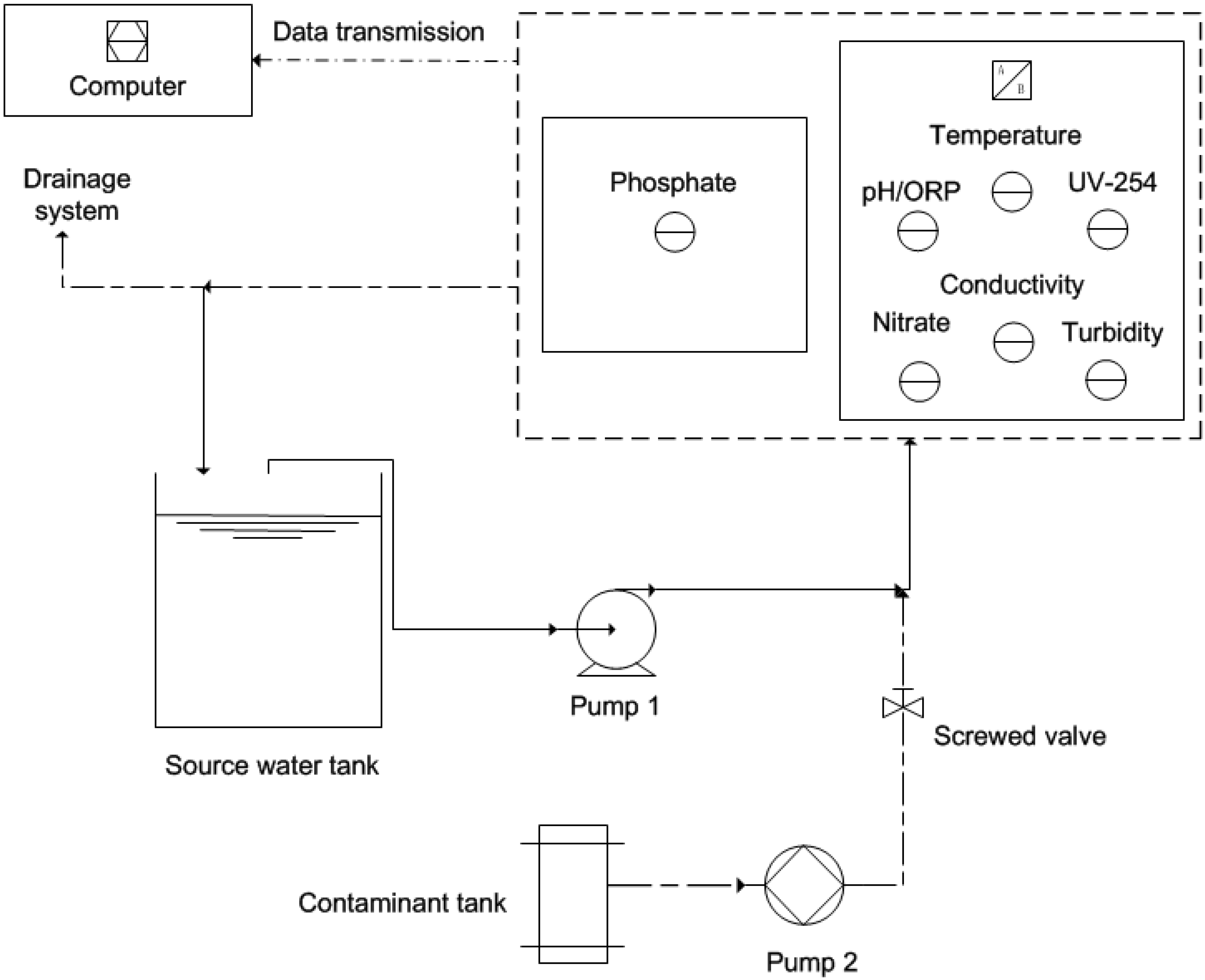
2.1. Pilot-Scale Contaminant Injection and Monitoring System

The pilot-scale system used in this study is a recirculating system simulator in the School of Environment Laboratory at Tsinghua University, Beijing, China. A process flow schematic of the pilot-scale system used for baseline establishment and single-pass contaminant tests is shown in Figure 1. The water tank is approximately 85 cm high with a diameter of 70 cm, and has a total capacity of 300 L. The tank is linked with the Guardian Blue early warning system [13] via a peristaltic pump at 0.5 L/min. The Guardian Blue early warning system, including Guardian Blue event monitor, agent library, water panel, TOC analyzer, and automatic sampler, is a system developed by Hach that detects, classifies, and alerts of a wide variety of threat contaminants. In this study, the system was only utilized as an online monitoring system. The system was operated in recirculation mode for baseline establishment. In this mode, 300 L source water flows through the eight sensors and back to the tank. The entire volume of water in the loop is replaced every 72 h if no contaminant test is conducted. Generally, the process of establishing baseline takes 4–6 h before any contaminant experiments can be carried out. When operating in single-pass contaminant mode, the target contaminant is injected into the pipe connecting the tank and sensors via another peristaltic pump. It is injected at a rate of 2–20 mL per minute depending on the concentration requirement. The water combined with contaminant flows through the sensors directly into a specific waste liquid bucket, avoiding pollution of the water in the tank.

Figure 1. A process flow schematic of the pilot-scale system.

Figure 1. A process flow schematic of the pilot-scale system.

2.2. Sensors Investigated

An online water quality monitoring system developed by Hach was utilized in this study. The system can measure the following eight parameters simultaneously and continuously: temperature, pH, turbidity, conductivity, oxidation reduction potential (ORP), UV-254, nitrate and phosphate. Table 1 shows a list of the parameters and the detailed information of their associated sensors.

Table 1. Detailed information of the parameters and sensors.

Parameter	Sensor Name	Measuring Range	Sensitivity	Measuring Interval
Temperature	DPD1R1-WDMP	−10–50 °C	±0.01 °C	1 min
pH	DPD1R1-WDMP	−2.00–14.00	±0.01	1 min
Turbidity	LXV423.99.10100	0.001–4,000 NTU	±0.001 NTU	1 min
Conductivity	D3725E2T-WDMP	0–2,000,000 us/cm	±1 us/cm	1 min
ORP	DRD1R5-WDMP	−1,500–1,500 mV	±0.5 mV	1 min
UV-254	LXG418.99.20000	0.01–60 1/m	±0.01 1/m	1 min
Nitrate	LXG.717.99.50000	0.1–100.0 mg/L	±0.1 mg/L	1 min
Phosphate	LXV422.99.20102	0.05–15 mg/L	±0.05 mg/L	5 min

Table 1. Detailed information of the parameters and sensors.

Parameter	Sensor Name	Measuring Range	Sensitivity	Measuring Interval
Temperature	DPD1R1-WDMP	−10–50 °C	±0.01 °C	1 min
pH	DPD1R1-WDMP	−2.00–14.00	±0.01	1 min
Turbidity	LXV423.99.10100	0.001–4,000 NTU	±0.001 NTU	1 min
Conductivity	D3725E2T-WDMP	0–2,000,000 us/cm	±1 us/cm	1 min
ORP	DRD1R5-WDMP	−1,500–1,500 mV	±0.5 mV	1 min
UV-254	LXG418.99.20000	0.01–60 1/m	±0.01 1/m	1 min
Nitrate	LXG.717.99.50000	0.1–100.0 mg/L	±0.1 mg/L	1 min
Phosphate	LXV422.99.20102	0.05–15 mg/L	±0.05 mg/L	5 min

2.3. Contaminants Investigated

The contaminant was determined according to statistical reports on water pollution incidents in urban water supply systems in China over the past 20 years. Glyphosate is known as a broad-spectrum systemic herbicide that is used to kill weeds, especially annual broadleaf weeds and grasses, and was selected as the target contaminant in this study. Specific quantities of the contaminant were injected into the system simulator.

2.4. Experimental Procedure

Sensors were calibrated in accordance with the manufacturer’s recommendations and were verified with a calibration check standard. Before the introduction of contaminants, the experimental system was kept running to establish a baseline. Sensor data were collected continuously and archived electronically to establish stable baseline conditions and to record sensor responses to injected contaminants. Data from the ORP, nitrate, temperature, pH, conductivity, turbidity and UV sensors were monitored and recorded every 1 min during the test period, while the phosphate sensor was recorded every 5 min. After the baseline was established, a specific concentration of contaminant was injected. Each contaminant injection took over 20–40 min to reach a stabilized reading. The sensors were then supplied with uncontaminated raw water and the responses returned to the baseline. The same contaminant, at a different concentration, was injected after sensor responses had returned to the baseline following the previous test [22].

2.5. Detection Method

In this study, it is assumed that multiple water quality sensors can respond to a contaminant simultaneously. The method detects contamination by exploring the correlative relationship between responses from multiple water quality sensors [21]. This relationship is evaluated using the correlation coefficient r, which is calculated by:

$$r_{xy}=\frac{{{\displaystyle \sum }}_{i=1}^n(x_i-\overline{x})(y_i-\overline{y})}{\sqrt{{{\displaystyle \sum }}_{i=1}^n{(x_i-\overline{x})}^2}\sqrt{{{\displaystyle \sum }}_{i=1}^n{(y_i-\overline{y})}^2}}$$

(1)

in which x and y refer to two separate water quality sensors, x, y ∈ (pH, ORP, UV, …); $\overline{x}$ and $\overline{y}$ stand for mathematical expectation; i goes from 1 to n and represents the index for window size. x_i and y_i stand for absolute values for corresponding sensors at time i. The number of data or window size is given by n. The window size is the number of past observations used to calculate the correlation coefficient. For each sensor, a new observation enters the sliding window at every time step t and the oldest observation exits (i.e., first in first out).

The value of r_xy is between −1 and 1. In this study, a correlation indicator C_xy is calculated using

$$C_{xy}=0,if\left|r_{xy}\right|<threshol{d}_{indicator},\text{or},r_{xy}=1$$

(2)

$$C_{xy}=1,ifthreshol{d}_{indicator}\le \left|r_{xy}\right|<1$$

(3)

A contamination alarm will be trigged if

$${\displaystyle \sum }_x^{\forall }{\displaystyle \sum }_y^{\forall }{\displaystyle \sum }{C}_{xy}\ge threshol{d}_{alarm}x\ne y,x,y\in \left\{pH,ORP,UV,\mathrm{...}\right\}$$

(4)

The value of threshold_indicator and threshold_alarm can be determined based on optimization analysis using data from experiments and real events.

The performance of the detection method is measured through detection time (DT), true positive rate (TPR), false positive rate (FPR) and false negative rate (FNR). DT is defined as the time difference between a contamination event taking place and when it is detected, and is evaluated by:

$$DT=T_1-T_0$$

(5)

where T₀ is the time when the contamination event occurs and T₁ is the time when the contamination event is detected. A smaller DT means the detection method is more effective and can detect contamination within a shorter time frame.

TPR, FPR and FNR can be calculated by [20]:

$$TP{R}_T=\frac{TP}{TP+FN}$$

(6)

$$FPR=\frac{FP}{FP+TN}$$

(7)

$$FNR=\frac{FN}{TP+FN}$$

(8)

where TP (true positive) is the detection of an actual event (alarm on); FP (false positive) refers to a routine operation being incorrectly classified as a contamination event (alarm on); TN (true negative) refers to a routine operation correctly being classified as such (alarm off); FN (false negative) means that an actual event is not detected (alarm off). TPR_T denotes the true positive rate after time T. A greater TPR means the method is more capable of detecting a real event, while a small FPR implies the method is less likely to classify a routine operation as an event.

In this study, the calculation is based on a 1 min step. A contaminant injection with period of t is assumed to be t contamination events. Within the period of contamination, if the method can detect the event, then TPR is used to evaluate the performance. The TPR_T is expressed as the true positive rate within the period from T to the end of injection. TPR₁ will be used as an evaluation indicator in this study unless otherwise indicated.

2.6. Parameter Optimization and Validation

Liu et al. [21] showed that this method was able to detect a contaminant event in a short time period and that the parameters had a significant impact on the detection performance. Likewise, in our study, an event can be detected if three parameters are given optimal values. Therefore, an optimization method can be used to obtain the best combination of threshold_indicator, threshold_alarm and window size. Non-Dominated Sorting Genetic Algorithm-II (NSGA-II) is a multi-objective optimization algorithm [23] used in recent studies [24,25,26]. It is computationally fast and has been shown to provide better coverage and maintain a better spread of solutions than other multi-objective algorithms.

The procedure of NSGA-II is summarized by the following steps: (1) generate the initial population randomly; (2) evaluate the performance of each chromosome and perform a fast non-domination sort; (3) produce the offspring through binary tournament selection, crossover and mutation; (4) form intermediate populations and perform a fast non-domination sort; (5) keep reproducing the new population until pre-set criteria is met. In this study, the minimum of “FNR” and the minimum of “FPR” were used as two fitness functions to evaluate the population of each generation. Values for NSGA-II operators were determined based on the literature [27] and listed in Table 2.

Table 2. Values of GA operators adopted.

Parameter Name	Value
Population	250
Generation number	200
Crossover rate	0.85
Mutation rate	0.05

Table 2. Values of GA operators adopted.

Parameter Name	Value
Population	250
Generation number	200
Crossover rate	0.85
Mutation rate	0.05

3. Results and Discussion

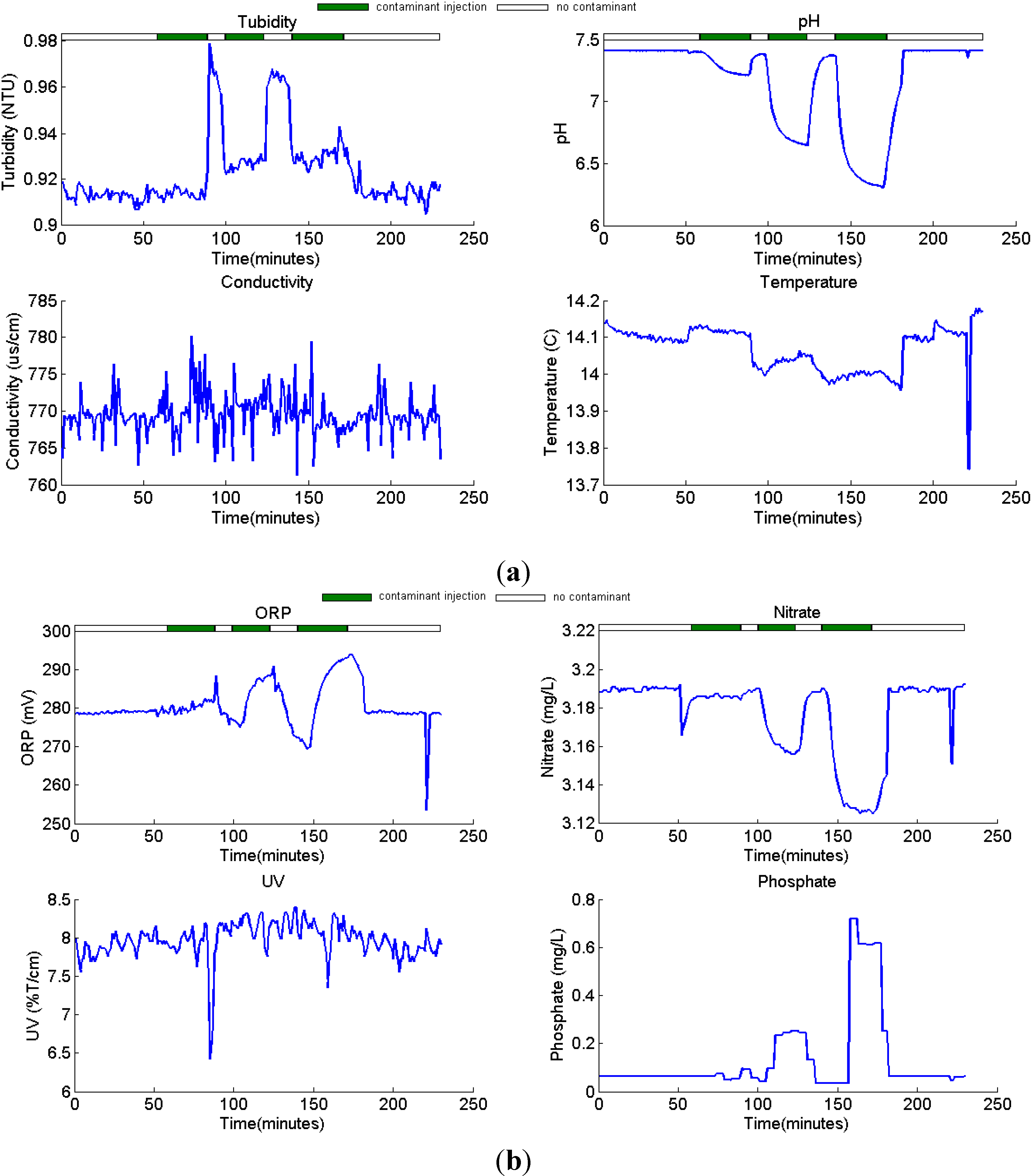
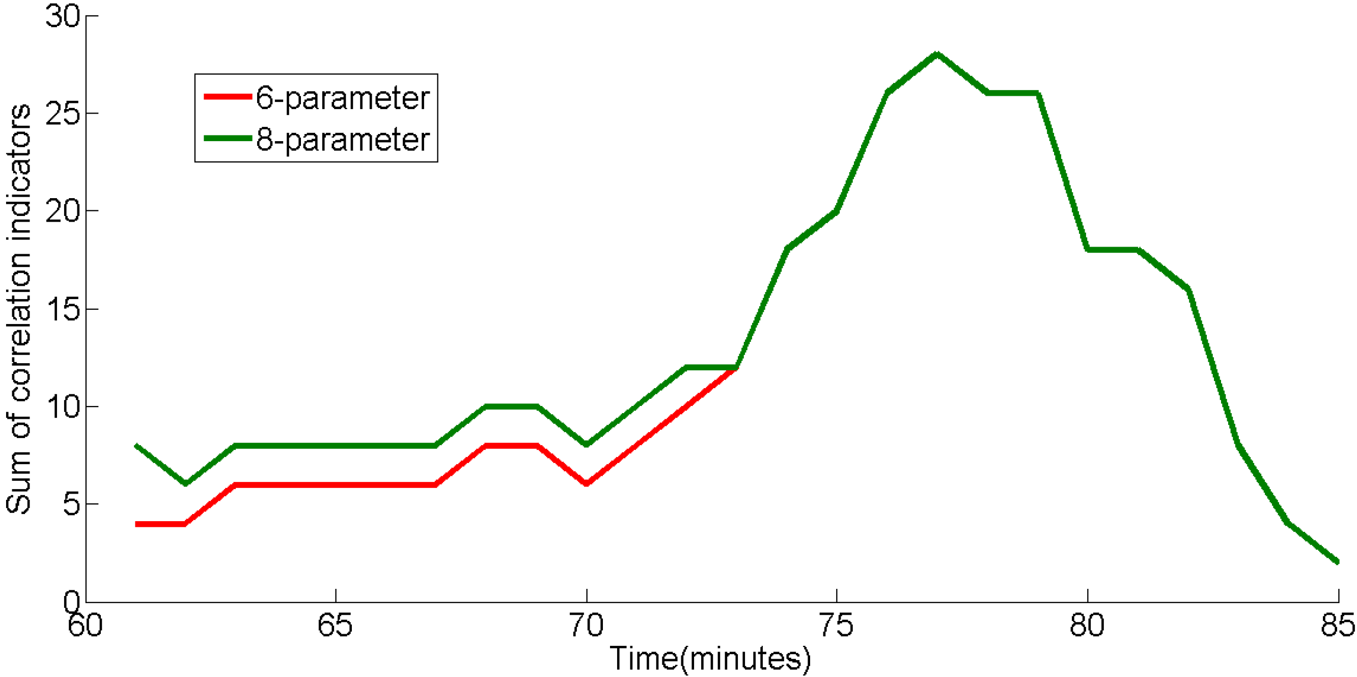
3.1. Correlative Responses

In this study, sensor response experiments for glyphosate with different concentrations were conducted. The results from the experiment involving glyphosate are shown in Figure 2a,b. In the experiment, glyphosate solutions with concentrations of 0.8 mg/L, 2.0 mg/L, and 4.0 mg/L were twice added in sequence. The data series obtained from the first and second time were recorded as series “glyphosate-A” and “glyphosate-B”. The “glyphosate-A” series is illustrated using solid green bars at the top of Figure 2. As shown in Figure 2, ORP and phosphate increase, while pH and nitrate decrease. The responses are mainly due to the introduction of glyphosate solution, as it is slightly acidic and has some oxidizing ability. The solution diluted the source water so nitrate shows a weak decrease. Conductivity and UV-254 sensors may have shown some response, but, if this is the case, the responses are hidden by the fluctuations from source water. Temperature has a clear increasing trend when the axes are enlarged, as shown in Figure 2a. Turbidity showed increases after both injections, which may appear to be a delayed reaction to the contaminant. However, these peaks in turbidity were not caused by the contaminant, but rather were an immediate result of a change in pump speed. Uncontaminated raw water is supplied to clean the pipe and system and the pump speed is increased in order to quickly return to baseline. The turbidity sensor is very sensitive to changes in water velocity, so it fluctuated as shown in the Figure 2a. Unexpected spikes are shown after the third injection in some sensor responses, mainly due to the sudden malfunction of the system.

For different contaminant concentrations, sensor responses show correlative relationships, especially for pH, nitrate, ORP and phosphate. This suggests the correlative response is caused by the introduction of contaminant and implies that this type of phenomenon can be utilized for detection of the presence of contamination. The magnitudes of the sensors’ responses were related to contaminant concentrations.

Figure 2. (a) Sensor responses (Turbidity, pH, Conductivity and Temperature) for glyphosate (concentrations: 0.8, 2.0, 4.0 mg/L); (b) Sensor responses (ORP, Nitrate, UV-254 and Phosphate) for glyphosate (concentrations: 0.8, 2.0, 4.0 mg/L).

Figure 2. (a) Sensor responses (Turbidity, pH, Conductivity and Temperature) for glyphosate (concentrations: 0.8, 2.0, 4.0 mg/L); (b) Sensor responses (ORP, Nitrate, UV-254 and Phosphate) for glyphosate (concentrations: 0.8, 2.0, 4.0 mg/L).

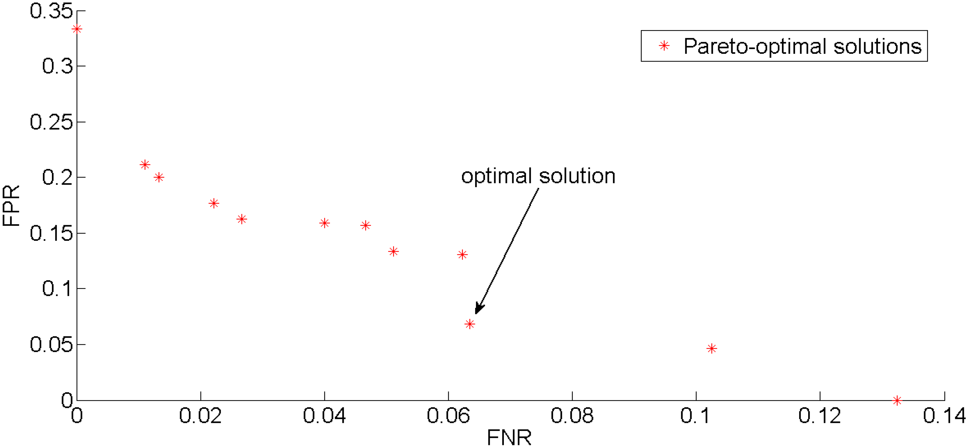
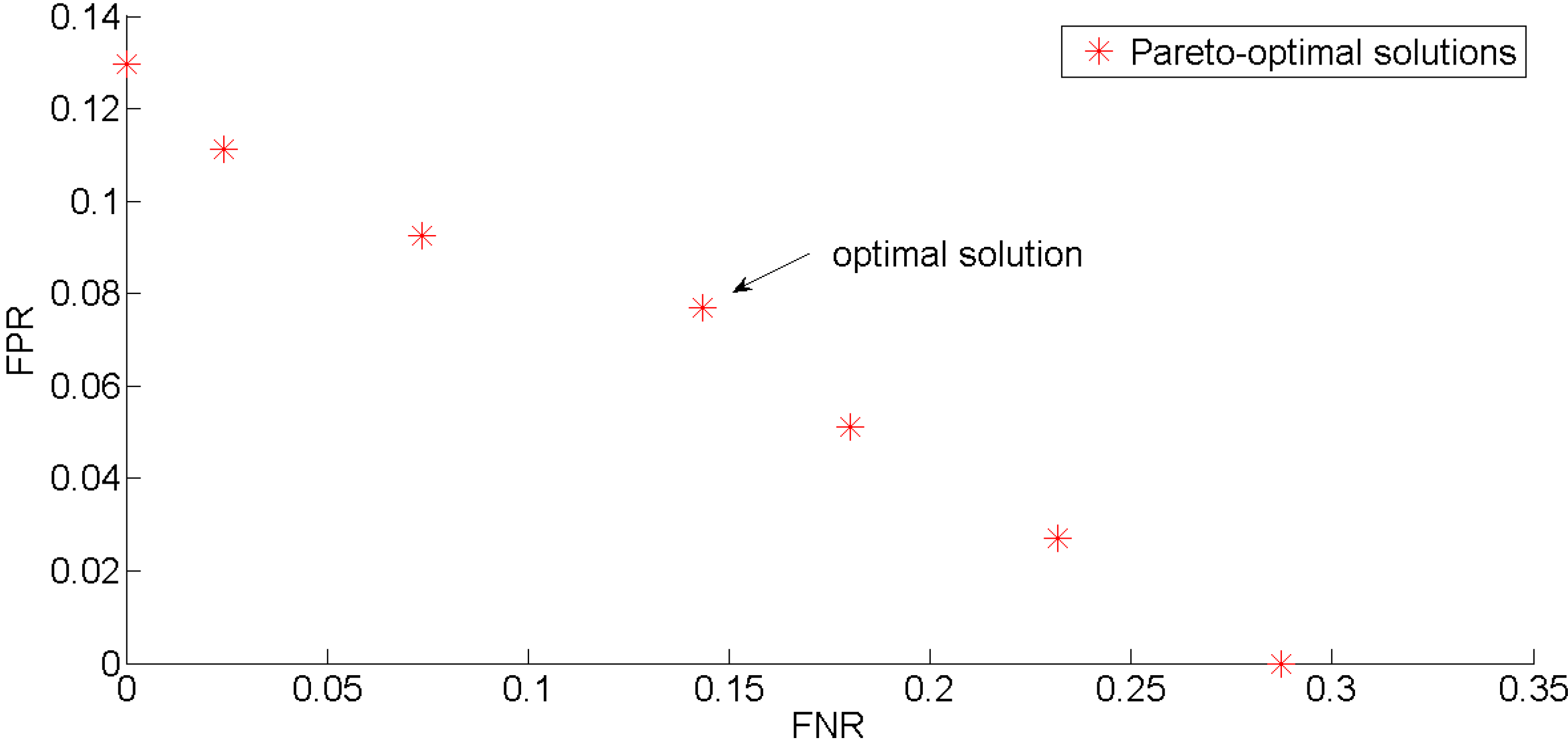
3.2. Parameter Optimization and Validation

The original data series for both glyphosate-A and glyphosate-B were each separated and regrouped into three individual new series, leaving a total of six new data series. Each new series contained 80–100 values. The first 60 values of the series were data for the no-contamination scenario, and the rest of the data were for the contamination scenario with different concentrations. The three new data series (A1, A2, A3) created from glyphosate-A were used as the calibration datasets and the other three new data series (B1, B2, B3) created from glyphosate-B were used as the validation datasets. The optimization results are shown in Figure 3.

Figure 3. The optimization results for glyphosate-A series with eight sensors.

Figure 3. The optimization results for glyphosate-A series with eight sensors.

As shown in Figure 3, although there were several solutions in the last generation, only one solution had the best performance, as pointed out with an arrow. The values of threshold_indicator, threshold_alarm and window size were 0.6912, 7, and 16, respectively. The TPR and FPR were 93.7% and 6.8%, respectively, which indicates that the proposed method has the ability to detect contamination events caused by glyphosate solution and that the accuracy is quite high.

The datasets used for validation were obtained from glyphosate-B data series, which contained three experiment data series with the same concentrations as glyphosate-A. For the parameters, the optimal values obtained from the calibration were used. Table 3 shows the results of validation. As shown in Table 3, the TPRs for the concentrations 0.8 mg/L, 2.0 mg/L and 4.0 mg/L were 95.5%, 100% and 100%, respectively. The FPR for all concentrations were 0%, which revealed excellent detection performance for glyphosate solution. The TPR of 100% indicated that the event could be detected one minute after the contamination occurred, which is very important in real events.

Table 3. The TPR and FPR performances of glyphosate-A and glyphosate-B series.

8-Sensor	Glyphosate-A			Glyphosate-B
Concentration	0.8 mg/L	2.0 mg/L	4.0 mg/L	0.8 mg/L	2.0 mg/L	4.0 mg/L
TPR	88.0%	96.3%	96.7%	95.5%	100.0%	100.0%
FPR	6.8%	6.8%	6.8%	0.0%	0.0%	0.0%

Table 3. The TPR and FPR performances of glyphosate-A and glyphosate-B series.

8-Sensor	Glyphosate-A			Glyphosate-B
Concentration	0.8 mg/L	2.0 mg/L	4.0 mg/L	0.8 mg/L	2.0 mg/L	4.0 mg/L
TPR	88.0%	96.3%	96.7%	95.5%	100.0%	100.0%
FPR	6.8%	6.8%	6.8%	0.0%	0.0%	0.0%

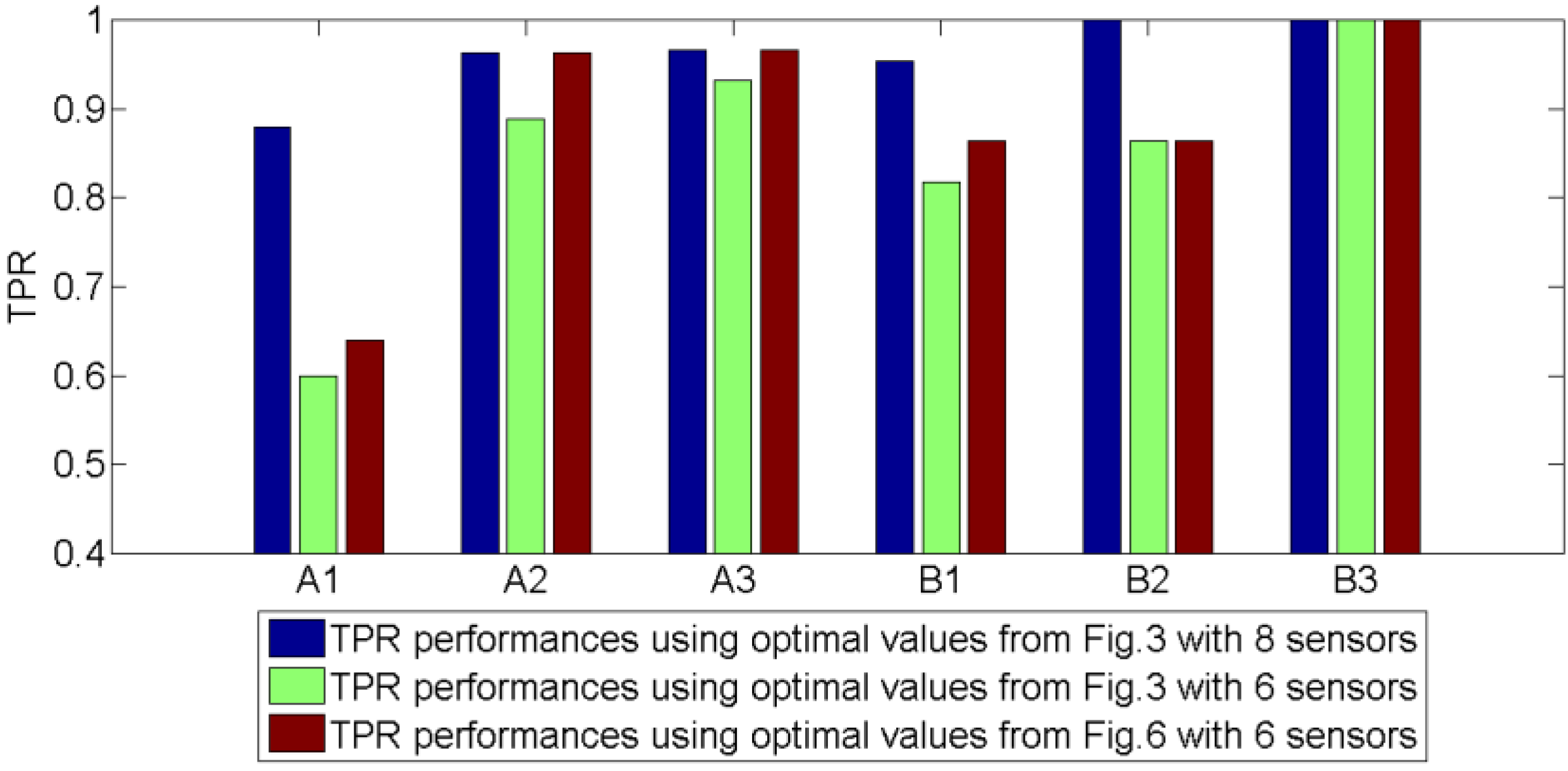
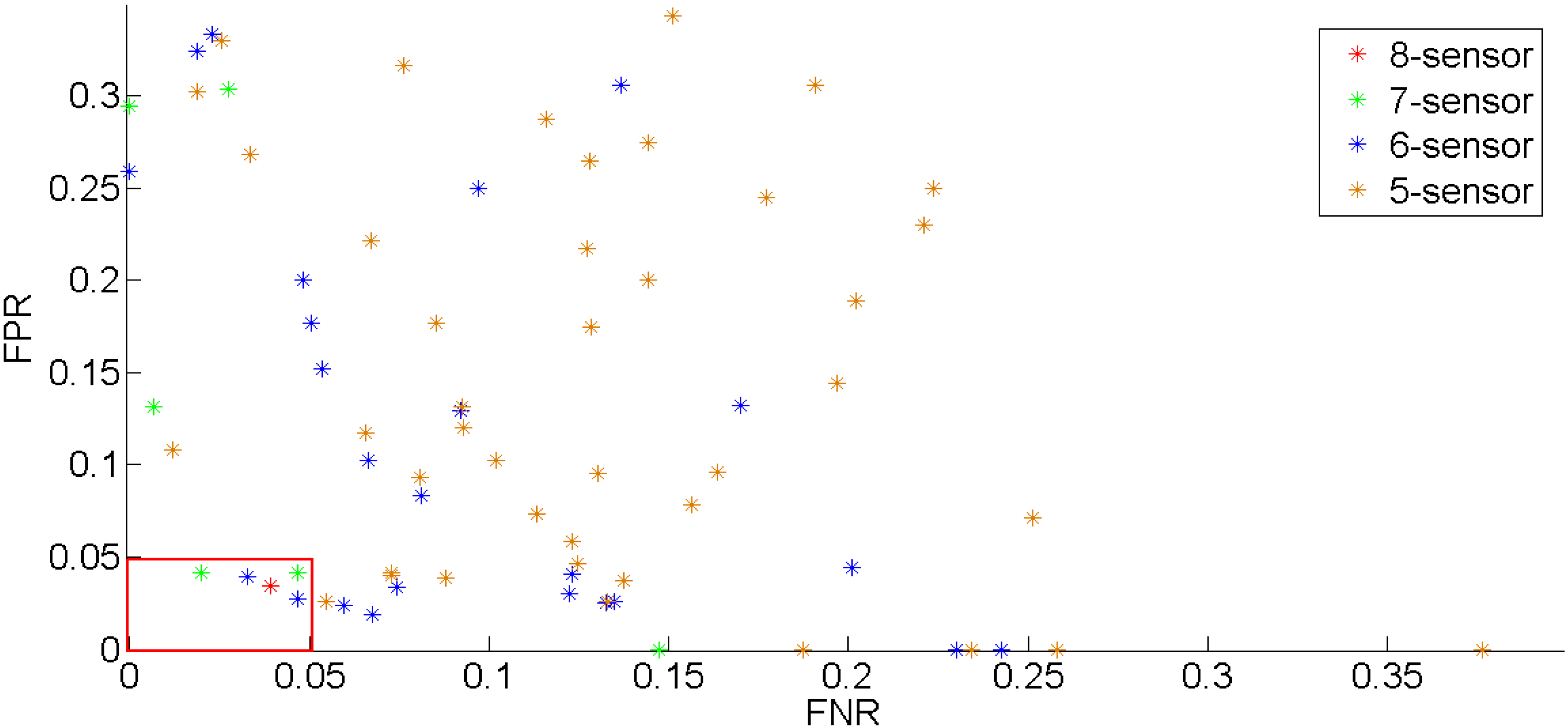
3.3. Sensors Selection

As can be seen from Figure 2, not all the sensors had obvious responses when contaminant was added. For example, the results from A-1 dataset show that turbidity and conductivity sensors both had weak responses. This leads to an interesting question: would the performance be affected if some sensors were removed? The correlation coefficients for each couple of sensors for the “contamination” scenario at the 85th minute were calculated and listed in Table 4.

Table 4. Correlation coefficients (contamination).

Sensor Name	Turbidity	pH	Conductivity	Temperature	ORP	Nitrate	UV	Phosphate
Turbidity	1.000	−0.447	−0.024	0.383	0.618	−0.424	−0.068	0.313
pH	−0.447	1.000	−0.093	−0.704	−0.947	0.832	−0.302	−0.625
Conductivity	−0.024	−0.093	1.000	0.167	−0.015	0.094	−0.091	0.021
Temperature	0.383	−0.704	0.167	1.000	0.688	−0.718	0.164	0.443
ORP	0.618	−0.947	−0.015	0.688	1.000	−0.781	0.216	0.544
Nitrate	−0.424	0.832	0.094	−0.718	−0.781	1.000	−0.399	−0.732
UV	−0.068	−0.302	−0.091	0.164	0.216	−0.399	1.000	0.274
Phosphate	0.313	−0.625	0.021	0.443	0.544	−0.732	0.274	1.000

Table 4. Correlation coefficients (contamination).

Sensor Name	Turbidity	pH	Conductivity	Temperature	ORP	Nitrate	UV	Phosphate
Turbidity	1.000	−0.447	−0.024	0.383	0.618	−0.424	−0.068	0.313
pH	−0.447	1.000	−0.093	−0.704	−0.947	0.832	−0.302	−0.625
Conductivity	−0.024	−0.093	1.000	0.167	−0.015	0.094	−0.091	0.021
Temperature	0.383	−0.704	0.167	1.000	0.688	−0.718	0.164	0.443
ORP	0.618	−0.947	−0.015	0.688	1.000	−0.781	0.216	0.544
Nitrate	−0.424	0.832	0.094	−0.718	−0.781	1.000	−0.399	−0.732
UV	−0.068	−0.302	−0.091	0.164	0.216	−0.399	1.000	0.274
Phosphate	0.313	−0.625	0.021	0.443	0.544	−0.732	0.274	1.000

From the results, it can be seen that the coefficients of turbidity and other sensor indicators at the 85th minute were smaller than the preset threshold. This suggests that the removal of turbidity would not affect the TPR performance at this time. Confirmation required further testing, so the turbidity and conductivity sensors were removed. The parameters obtained from the calibration were used and the TPR performances were shown in Figure 4. The results showed that the FPR for glyphosate-A and glyphosate-B were 4.6% and 0%, respectively, which indicated that the performance did not change much, and was even improved. However, the TPR was greatly impacted, especially for the lowest concentrations.

Figure 4. Comparison of TPR performances.

Figure 4. Comparison of TPR performances.

Figure 5 shows the sum of correlation indicators at each time step that contaminant was added (from the 61st to 85th minutes in A-1 dataset). It revealed two situations in which eight sensors and six sensors were used. The sum of correlation indicators for eight sensors was higher than that for six sensors for the first ten minutes. This indicates that the turbidity and conductivity sensors responded to the injection of glyphosate, although this was not clear from the change of the original data series in Figure 2. Figure 5 also reveals that the turbidity and conductivity sensors made little contribution to event detection after the concentration stabilized.

Figure 5. The sum of correlation indicators at each time step in two situations.

Figure 5. The sum of correlation indicators at each time step in two situations.

Another optimization was conducted in order to find the optimal parameters when using six sensors. The three new data series created from glyphosate-A were again used as the calibration datasets and the other three new data series created from glyphosate-B were used as the validation datasets. The optimal values of threshold_indicator, threshold_alarm and window size were 0.6111, 7, and 21, respectively. The TPR and FPR results are shown in Figure 4, Figure 6 and Table 5. It can be seen that the average TPR and FPR for the six data series were 88.3% and 3.8%, respectively. This was lower than, but close to, the performance with eight sensors. The detection method appeared to adapt well as the number of monitoring sensors changed. To confirm this, 93 (1 + 8 + 28 + 56) sensor combinations were created and optimized. The number of sensors ranged from five to eight. For each combination, there were several optimal solutions with different FNR and FPR. Here the distance from each solution point to the base point was used as a calculation method to choose the best solution. The best solution points for each combination are shown in Figure 7.

Figure 6. The optimization results for glyphosate-A series with six sensors.

Figure 6. The optimization results for glyphosate-A series with six sensors.

Table 5. The TPR and FPR performances of glyphosate-A and glyphosate-B series.

6-Sensor	Glyphosate-A			Glyphosate-B
Concentration	0.8 mg/L	2.0 mg/L	4.0 mg/L	0.8 mg/L	2.0 mg/L	4.0 mg/L
TPR	64.0%	96.3%	96.7%	86.4%	86.4%	100.0%
FPR	7.6%	7.6%	7.6%	0.0%	0.0%	0.0%

Table 5. The TPR and FPR performances of glyphosate-A and glyphosate-B series.

6-Sensor	Glyphosate-A			Glyphosate-B
Concentration	0.8 mg/L	2.0 mg/L	4.0 mg/L	0.8 mg/L	2.0 mg/L	4.0 mg/L
TPR	64.0%	96.3%	96.7%	86.4%	86.4%	100.0%
FPR	7.6%	7.6%	7.6%	0.0%	0.0%	0.0%

Figure 7. The result for different sensor deployment.

Figure 7. The result for different sensor deployment.

Each point in Figure 7 represents the result of one sensor combination. The red one corresponds to the eight-sensor combination, while the green, blue and yellow ones correspond to seven-sensor, six-sensor and five-sensor combinations, respectively. The points in the red rectangle represent the optimal combinations when FNR and FPR were less than 5%. One point is the eight-sensor combination, two points are seven-sensor combinations and two points are six-sensor combinations. Although there is no five-sensor combination point inside the rectangle, the closest five-sensor point also showed a reasonable performance with an FNR of 5.4% and FPR of 2.6%. It is worth noting that the detection method was able to adapt well as the number of monitoring sensors decreased from eight to five, as expected. Table 6 listed the sensors (parameters) used in different optimal solutions.

Table 6. Sensors used in each optimal solution.

Number of Sensors	Sensor Names
7	Turbidity, pH, conductivity, temperature, ORP, nitrate, UV-254
7	Turbidity, pH, Conductivity, ORP, Nitrate, UV-254, Phosphate
6	Turbidity, pH, Conductivity, ORP, Nitrate, Phosphate
6	Turbidity, pH, Temperature, ORP, Nitrate, Phosphate
5	Turbidity, pH, ORP, Nitrate, Phosphate

Table 6. Sensors used in each optimal solution.

Number of Sensors	Sensor Names
7	Turbidity, pH, conductivity, temperature, ORP, nitrate, UV-254
7	Turbidity, pH, Conductivity, ORP, Nitrate, UV-254, Phosphate
6	Turbidity, pH, Conductivity, ORP, Nitrate, Phosphate
6	Turbidity, pH, Temperature, ORP, Nitrate, Phosphate
5	Turbidity, pH, ORP, Nitrate, Phosphate

From the results of Table 6, it can also be seen that the removed sensors were mainly UV-254, conductivity, or temperature. Figure 2 shows that these sensors did not change visibly in response to contamination events, whereas responses of the pH, ORP, nitrate and phosphate sensors were very strong. It can also be seen from Figure 7 that the points representing fiv-sensor combinations where generally further from the origin of the graph (i.e., optimal point) than the points representing six-sensor combinations. This was also true for six-sensor points when compared with seven-sensor points. More sensors help to improve the detection performance but also increase costs. However, as mentioned previously, appropriate selection of the sensors results in good performance when five, six, seven, or eight sensors are used. In another words, utilizing fewer sensors in areas where reducing costs is important would also lead to excellent detection performance.

4. Conclusions

In this study, a method utilizing the correlative relationship between multiple sensors was optimized. The results from the experiment and analysis showed that the method with suitable optimization could detect a glyphosate contamination in less than 5 min after the introduction of contaminant using responses from online water quality sensors. The average TPR₁ was 95.5%.

The study discussed the impact of the number of sensors on detection performance. The results showed that if the number of sensors was reduced from eight to five, the TPR performance was still good. This indicates that the method is flexible and can be applied using a smaller number of sensors to reduce monitoring costs.

References

1. Gullick, R.W.; Grayman, W.M.; Deininger, R.; Males, R.M. Design of early warning monitoring systems for source waters. J. Am. Water Work. Assoc. 2003, 95, 58–72. [Google Scholar]
2. Storey, M.V.; van der Gaag, B.; Burns, B.P. Advances in on-line drinking water quality monitoring and early warning systems. Water Res. 2011, 45, 741–747. [Google Scholar] [CrossRef] [PubMed]
3. Hasan, J.; States, S.; Deininger, R. Safeguarding the security of public water supplies using early warning systems: A brief review. J. Contemp. Water Res. Educ. 2004, 129, 27–33. [Google Scholar] [CrossRef]
4. Hawkins, P.R.; Novic, S.; Cox, P.; Neilan, B.A.; Burns, B.P.; Shaw, G.; Wickramasinghe, W.; Peerapornpisal, Y.; Ruangyuttikarn, W.; Itayama, T.; et al. A review of analytical methods for assessing the public health risk from microcystin in the aquatic environment. J. Water Supply Res. Technol. 2005, 54, 509–518. [Google Scholar]
5. Henderson, R.K.; Baker, A.; Murphy, K.R.; Hamblya, A.; Stuetz, R.M.; Khan, S.J. Fluorescence as a potential monitoring tool for recycled water systems: A review. Water Res. 2009, 43, 863–881. [Google Scholar] [CrossRef] [PubMed]
6. Marshall, C.P.; Leuko, S.; Coyle, C.M.; Walter, M.R.; Burns, B.P.; Neilan, B.A. Carotenoid analysis of halophilic archaea by resonance raman spectroscopy. Astrobiology 2007, 7, 631–643. [Google Scholar] [CrossRef] [PubMed]
7. Pomati, F.; Burns, B.P.; Neilan, B.A. Identification of an Na+-dependent transporter associated with saxitoxin-producing strains of the cyanobacterium anabaena circinalis. Appl. Environ. Microbiol. 2004, 70, 4711–4719. [Google Scholar] [CrossRef] [PubMed]
8. De Hoogh, C.J.; Wagenvoort, A.J.; Jonker, F.; van Leerdam, J.A.; Hogenboom, A.C. Hplc-Dad and Q-TOF MS techniques identify cause of Daphnia biomonitor alarms in the River Meuse. Environ. Sci. Technol. 2006, 40, 2678–2685. [Google Scholar] [CrossRef] [PubMed]
9. Jeon, J.; Kim, J.H.; Lee, B.C.; Kim, S.D. Development of a new biomonitoring method to detect the abnormal activity of Daphnia magna using automated Grid Counter device. Sci. Total Environ. 2008, 389, 545–556. [Google Scholar] [CrossRef] [PubMed]
10. McKenna, S.A.; Wilson, M.; Klise, K.A. Detecting changes in water quality data. J. Am. Water Work. Assoc. 2008, 100, 74–85. [Google Scholar]
11. Hall, J.; Zaffiro, A.D.; Marx, R.B.; Kefauver, P.C.; Krishnan, E.R.; Herrmann, J.G. On-Line water quality parameters as indicators of distribution system contamination. J. Am. Water Work. Assoc. 2007, 99, 66–77. [Google Scholar]
12. Yang, Y.J.; Haught, R.C.; Goodrich, J.A. Real-Time contaminant detection and classification in a drinking water pipe using conventional water quality sensors: Techniques and experimental results. J. Environ. Manag. 2009, 90, 2494–2506. [Google Scholar] [CrossRef]
13. Kroll, D.; King, K. The utilization on-line of common parameter monitoring as a surveillance tool for enhancing water security. Spec. Publ. R. Soc. Chem. 2006, 302, 89–98. [Google Scholar]
14. Liu, S.; Che, H.; Smith, K.; Chang, T. A real time method of contaminant classification using conventional water quality sensors. J. Environ. Manag. 2015, 154, 13–21. [Google Scholar] [CrossRef]
15. Hart, D.; McKenna, S.A.; Klise, K.; Cruz, V.; Wilson, M. CANARY: A water quality event detection algorithm development tool. In Proceedings of the World Environmental and Water Resources Congress, Tampa, FL, USA, 15–19 May 2007; pp. 1–9.
16. Klise, K.A.; McKenna, S.A. Water quality change detection: Multivariate algorithms. In Proceedings of the Defense and Security Symposium, International Society for Optics and Photonics, Kissimmee, FL, USA, 17 April 2006.
17. Allgeier, S.; Murray, R.; Mckenna, S.; Shalvi, D. Overview of Event Detection Systems for WaterSentinel; United States Environmental Protection Agency: Washington, DC, USA, 12 December 2005. [Google Scholar]
18. Raciti, M.; Cucurull, J.; Nadjm-Tehrani, S. Anomaly detection in water management systems. In Critical Infrastructure Protection; Springer: Berlin/Heidelberg, Germany, 2012; pp. 98–119. [Google Scholar]
19. Perelman, L.; Arad, J.; Housh, M.; Ostfeld, A. Event detection in water distribution systems from multivariate water quality time series. Environ. Sci. Technol. 2012, 46, 8212–8219. [Google Scholar] [CrossRef] [PubMed]
20. Arad, J.; Housh, M.; Perelman, L.; Ostfeld, A. A dynamic thresholds scheme for contaminant event detection in water distribution systems. Water Res. 2013, 47, 1899–1908. [Google Scholar] [CrossRef] [PubMed]
21. Liu, S.; Che, H.; Smith, K.; Chen, L. Contamination event detection using multiple types of conventional water quality sensors in source water. Environ. Sci. Process. Impacts 2014, 16, 2028–2038. [Google Scholar] [CrossRef] [PubMed]
22. Che, H.; Liu, S. Contaminant detection using multiple conventional water quality sensors in an early warning system. Procedia Eng. 2014, 89, 479–487. [Google Scholar] [CrossRef]
23. Deb, K.; Pratap, A.; Agarwal, S.; Meyarivan, T. A fast and elitist multiobjective genetic algorithm: NSGA-II. IEEE Trans. Evol. Comput. 2002, 6, 182–197. [Google Scholar] [CrossRef]
24. Sweetapple, C.; Fu, G.T.; Butler, D. Multi-Objective optimisation of wastewater treatment plant control to reduce greenhouse gas emissions. Water Res. 2014, 55, 52–62. [Google Scholar] [CrossRef] [PubMed] [Green Version]
25. Zhang, C.; Zhu, X.P.; Fu, G.T.; Zhou, H.C.; Wang, H. The impacts of climate change on water diversion strategies for a water deficit reservoir. J. Hydroinform. 2014, 16, 872–889. [Google Scholar] [CrossRef]
26. Berardi, L.; Giustolisi, O.; Savic, D.A.; Kapelan, Z. An effective multi-objective approach to prioritisation of sewer pipe inspection. Water Sci. Technol. 2009, 60, 841–850. [Google Scholar] [CrossRef] [PubMed]
27. Liu, S.M.; Butler, D.; Brazier, R.; Heathwaite, L.; Khu, S.T. Using genetic algorithms to calibrate a water quality model. Sci. Total. Environ. 2007, 374, 260–272. [Google Scholar] [CrossRef] [PubMed]