Impacts of Climate Change on Mean Annual Water Balance for Watersheds in Michigan, USA

Abstract

Evaluation of water balance at the watershed scale is a fundamental step for estimating streamflow in watersheds. Mean annual water balance of 17 watersheds across Michigan were evaluated by comparing observed streamflow with simulated streamflow estimated using Fu’s Equation, which is based on the Budyko Hypothesis. The Budyko Hypothesis describes mean annual water balance as a function of available water and energy. Impact of long-term climatic controls (e.g., precipitation, potential evapotranspiration (ET_P)) on mean annual water balance was also investigated with Fu’s Equation. Results indicated that observed streamflow ranged from 237 to 529 mm per year, with an average of 363 mm per year in the study watersheds during 1967–2011. On average, 40% of long-term precipitation in the study watersheds was converted into surface runoff. The performance of Fu’s Equation in estimating mean annual streamflow resulted in Root Mean Square Error (RMSE) value of 64.1 mm/year. Mean annual streamflow was sensitive to changes in mean annual precipitation, and less sensitive to changes in mean annual ET_p in the watersheds. With the increase of baseflow index (BFI), mean annual streamflow was less sensitive to climate change. Overall, different contributions of baseflow to streamflow modified the impact of climate controls on mean annual water balance in the baseflow-dominated watersheds.

1. Introduction

Water balance refers to the quantitative description of the hydrologic cycle. It is often expressed with water balance equations (i.e., the relationship between input and output of water through an area during a given time period). A water balance model is generally selected based on specific project requirements, available data, and the application scope of the model. Empirical data of catchment all over the world indicate that the long-term water balance is primarily controlled by water supply (i.e., precipitation) and energy demand (i.e., potential evapotranspiration), these relatively simple models have been developed [1,2,3,4]. The Budyko Hypothesis, the relationship between actual evapotranspiration ratio (i.e., the ratio of actual evapotranspiration to precipitation) and climate aridity index (i.e., the ratio of potential evapotranspiration to precipitation), is a useful tool to examine watershed water balance and to investigate the effects of climate change and watershed characteristics on the hydrologic cycle [5,6,7,8,9].

Although a variety of equations satisfying the Budyko Hypothesis can be found in previous studies [4,10,11,12,13,14,15], Budyko-type equations with optimizable parameters are particularly useful for modeling mean annual and annual water balance in individual watersheds [16,17]. Fu’s Equation, an analytical solution of the Budyko Hypothesis, is a one-parameter conceptual model derived from dimensional analysis and mathematical reasoning (rather than a simple empirical fit to hydrologic data) [12]. Fu’s Equation can provide reasonable results for estimating mean annual and annual water balances in most individual watersheds [15,18]. Based on its simplicity, Fu’s Equation was utilized in this study to evaluate long-term water balance at catchment scales.

Long-term water balance is affected by climatic controls (i.e., precipitation (P) and potential evapotranspiration (ET_p)) according to the Budyko Hypothesis. The Budyko water balance approach for estimating the climatic sensitivity has been widely applied in previous studies [8,19,20,21,22]. However, studies relating groundwater (e.g., baseflow) to Budyko Hypothesis were relatively rare. Wang et al. [23] explored the effects of soil texture and groundwater (e.g., baseflow) on mean annual and annual water balances of watersheds in the Nebraska Sand Hills, based on the Budyko Hypothesis. Results suggested that soil texture may greatly modify the influence of climate on regional water balance; and a water storage term needed to be included in the Budyko Hypothesis on annual time scales when baseflow contribution was significant.

This study is a continuous work based on [24], in which 17 watersheds have been used to develop regression equations for estimating baseflow and baseflow index. On average, baseflow accounted for 70% of the total streamflow in those 17 watersheds [24]. The specific objective of this study were to (1) test the applicability of Fu’s Equation in estimating mean annual water balances for 17 watersheds in Michigan; and (2) investigate the relationship between baseflow and climatic sensitivity in Michigan watersheds using Fu’s Equation. The evaluation of watershed water balance in this study was intended to provide quantitative insight into water balance response to climatic factors in various watersheds, especially in baseflow-dominated watersheds.

2. Materials and Methods

2.1. Data Used

Watershed characteristics and meteorological variables used for water balance calculations in this study include: Watershed location (latitude of the gaging stations), annual precipitation (P), annual streamflow (Q), maximum daily temperature (averaged over all days in the month) (T_max) and minimum daily temperature (averaged over all days in the month) (T_min), and solar radiation (R_a). Annual precipitation and monthly average maximum and minimum daily temperature for the study watersheds were derived from Parameter-elevation Regressions on Independent Slopes Model (PRISM) climate analysis system [25]. All datasets mentioned above were compiled using ArcGIS 10 [26] for a period of 1967 to 2011. Streamflow data were obtained from USGS (United States Geological Survey) gaging stations [27]. The Eckhardt filter method [28] in Web-based Hydrograph Analysis Tool program was used to partition daily streamflow records into direct runoff and baseflow for the study period of 1967 to 2011 [29]. The default recess constant and BFI_max values of 0.98 and 0.8 were employed, respectively. The specific principle of the recursive partitioning algorithm was shown in detail in the study by Zhang et al. [24]. Then, baseflow index (BFI) was calculated by dividing mean annual baseflow by mean annual streamflow to quantify groundwater contributions to streamflow in the 17 study watersheds.

2.2. Potential Evapotranspiration Calculation

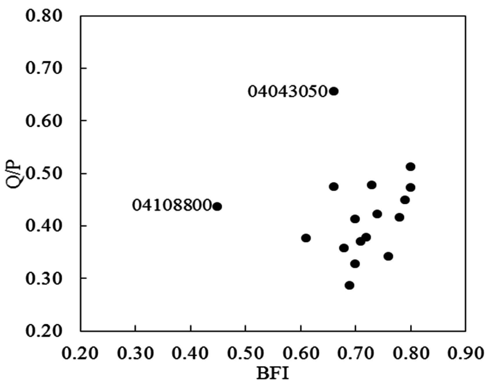
The Hargreaves method [30] is based on time series of average maximum and minimum temperature data and solar radiation. It has been widely used to estimate ET_P in previous studies [31,32,33]. The equation can be expressed as [30]:

$${\text{ET}}_{\text{p}}\text{ = 0}{\text{.0023R}}_{\text{a}}\left(\frac{{\text{T}}_{\text{max}}{\text{+T}}_{\text{min}}}{\text{2}}\text{+17.8}\right)\sqrt{\left({\text{T}}_{\text{max}}{\text{-T}}_{\text{min}}\right)}$$

(1)

where ET_p is the potential evapotranspiration, mm/d; T_max and T_min are the maximum monthly temperature and minimum monthly temperature, respectively, °C; R_a is the extraterrestrial solar radiation, mm/d.

Daily solar radiation of individual gaging stations was calculated based on the latitude values (shown in Table 1) using the calculator of extraterrestrial solar radiation tool [34].Monthly time series of average maximum and minimum temperature data along with the computed solar radiation were used to calculate monthly ET_p in mm/d using Equation (1). Annual ET_p in the study watersheds was derived from summing monthly ET_p of each year.

Table 1. Gaging stations and water balance components of seventeen watersheds in Michigan.

Gaging Station ID	Station Name and Location	Latitude	Delineated Area (km2)	P (mm/yr)	ETP (mm/yr)	Q (mm/yr)	ETa (mm/yr)	$\frac{{\text{ET}}_{\text{p}}}{\text{P}}$	Q/P	$\frac{{\text{ET}}_{\text{a}}}{\text{P}}$	BFI
04040500	Sturgeon River near Sidnaw	46.584	429.8	878	832	416	462	0.95	0.47	0.53	0.66
04043050	Trap Rock River near Lake Linden	47.229	77.1	807	757	529	278	0.94	0.66	0.34	0.66
04045500	Tahquamenon River near Paradise	46.575	1960.6	828	832	395	432	1.00	0.48	0.52	0.73
04057510	Sturgeon River near Nahma Junction	45.943	475.4	826	866	348	478	1.05	0.42	0.58	0.74
04059500	Ford River near Hyde	45.755	1156.8	776	843	278	499	1.09	0.36	0.64	0.68
04096405	Sturgeon River at Wolverine	45.274	454.7	850	906	402	449	1.07	0.47	0.53	0.80
04105000	Manistee River near Sherman	44.436	2241.9	835	912	428	407	1.09	0.51	0.49	0.80
04105700	Pere Marquette River at Scottville	43.945	1787.7	883	963	396	487	1.09	0.45	0.55	0.79
04108600	Macatawa River at State Road near Zeeland	42.779	172.9	930	951	406	525	1.02	0.44	0.56	0.45
04108800	Rabbit River near Hopkins	42.642	174.9	938	934	307	631	1.00	0.33	0.67	0.70
04117500	Thornapple River near Hastings	42.616	1063.4	886	972	328	558	1.10	0.37	0.63	0.71
04122500	Augusta Creek Near Augusta	42.353	95.2	949	1003	394	555	1.06	0.42	0.58	0.78
04124000	Battle Creek at Battle Creek	42.331	710	888	970	335	552	1.09	0.38	0.62	0.72
04127997	St. Joseph River at Burlington	42.103	530.7	932	957	319	613	1.03	0.34	0.66	0.76
04161580	Stony Creek near Romeo	42.801	61.7	826	925	237	589	1.12	0.29	0.71	0.69
04164000	Clinton River near Fraser	42.578	1188.3	823	943	340	483	1.15	0.41	0.59	0.70
04166100	River Rouge at Southfield	42.448	225.3	815	954	307	509	1.17	0.38	0.62	0.61

Table 1. Gaging stations and water balance components of seventeen watersheds in Michigan.

Gaging Station ID	Station Name and Location	Latitude	Delineated Area (km2)	P (mm/yr)	ETP (mm/yr)	Q (mm/yr)	ETa (mm/yr)	$\frac{{\text{ET}}_{\text{p}}}{\text{P}}$	Q/P	$\frac{{\text{ET}}_{\text{a}}}{\text{P}}$	BFI
04040500	Sturgeon River near Sidnaw	46.584	429.8	878	832	416	462	0.95	0.47	0.53	0.66
04043050	Trap Rock River near Lake Linden	47.229	77.1	807	757	529	278	0.94	0.66	0.34	0.66
04045500	Tahquamenon River near Paradise	46.575	1960.6	828	832	395	432	1.00	0.48	0.52	0.73
04057510	Sturgeon River near Nahma Junction	45.943	475.4	826	866	348	478	1.05	0.42	0.58	0.74
04059500	Ford River near Hyde	45.755	1156.8	776	843	278	499	1.09	0.36	0.64	0.68
04096405	Sturgeon River at Wolverine	45.274	454.7	850	906	402	449	1.07	0.47	0.53	0.80
04105000	Manistee River near Sherman	44.436	2241.9	835	912	428	407	1.09	0.51	0.49	0.80
04105700	Pere Marquette River at Scottville	43.945	1787.7	883	963	396	487	1.09	0.45	0.55	0.79
04108600	Macatawa River at State Road near Zeeland	42.779	172.9	930	951	406	525	1.02	0.44	0.56	0.45
04108800	Rabbit River near Hopkins	42.642	174.9	938	934	307	631	1.00	0.33	0.67	0.70
04117500	Thornapple River near Hastings	42.616	1063.4	886	972	328	558	1.10	0.37	0.63	0.71
04122500	Augusta Creek Near Augusta	42.353	95.2	949	1003	394	555	1.06	0.42	0.58	0.78
04124000	Battle Creek at Battle Creek	42.331	710	888	970	335	552	1.09	0.38	0.62	0.72
04127997	St. Joseph River at Burlington	42.103	530.7	932	957	319	613	1.03	0.34	0.66	0.76
04161580	Stony Creek near Romeo	42.801	61.7	826	925	237	589	1.12	0.29	0.71	0.69
04164000	Clinton River near Fraser	42.578	1188.3	823	943	340	483	1.15	0.41	0.59	0.70
04166100	River Rouge at Southfield	42.448	225.3	815	954	307	509	1.17	0.38	0.62	0.61

2.3. Water Balance Modeling Based on Budyko Hypothesis

Budyko [3,4] reported that mean annual ET_a is primarily controlled by available water and energy. Budyko Hypothesis is a model that represents ET_a/P ratio as a function of climatic aridity index. It can be expressed as:

$$\frac{{\text{ET}}_{\text{a}}}{\text{P}}\text{ = F}\left(\frac{{\text{ET}}_{\text{p}}}{\text{P}}\right)$$

(2)

where ET_a/P is the ET_a ratio; ET_p/P is the climate aridity index; F is an empirical function.

The relationship presented in Equation (2) assumes that average annual P and ET_p are the dominant factors controlling mean annual ET_a. Budyko’s Equation can be represented as [4]:

$$\frac{{\text{ET}}_{\text{a}}}{\text{P}}\text{ = }{\left\{\frac{{\text{ET}}_{\text{P}}}{\text{P}}\text{tanh}\left(\frac{\text{P}}{{\text{ET}}_{\text{P}}}\right)\left[\text{1}-\text{cosh}\left(\frac{{\text{ET}}_{\text{P}}}{\text{P}}\right)\text{+sinh}\left(\frac{{\text{ET}}_{\text{P}}}{\text{P}}\right)\right]\right\}}^{\text{0.5}}$$

(3)

To incorporate the effects of factors such as vegetation, soil water storage, and rainfall seasonality, among others, on water balance, Budyko-type equations with adjustable parameters have been developed for various applications [5,12,13,14,23]. Fu’s Equation contains a parameter (w, w > 1) that represents the combined effects of climatic conditions (e.g., rainfall seasonality) and catchment characteristics (e.g., vegetation cover, soil properties and catchment topography) on the water balance [15,35]. Fu’s Equation can be expressed as:

$$\frac{{\text{ET}}_{\text{a}}}{\text{P}}\text{ = 1+}\frac{{\text{ET}}_{\text{P}}}{\text{P}}-{\left[\text{1+}{\left(\frac{{\text{ET}}_{\text{p}}}{\text{P}}\right)}^{\text{w}}\right]}^{\frac{\text{1}}{\text{w}}}$$

(4)

In this study, ET_a was derived from water balance equation (i.e., ET_a = P − Q) and w was fitted using SOLVER in Microsoft Excel 2010. The average fitted w (w = 1.95) was utilized for calculating mean annual Q using the following equation:

$$\text{Q = P}{\left[\text{1+}{\left(\frac{{\text{ET}}_{\text{p}}}{\text{P}}\right)}^{\text{w}}\right]}^{\frac{\text{1}}{\text{w}}}-{\text{ET}}_{\text{p}}$$

(5)

RMSE (Root Mean Square Error) was used to evaluate the performance of Fu’s Equation (w = 1.95) in the estimation of mean annual streamflow of 17 watersheds in Michigan. The corresponding equation was expressed as:

$$\text{RSME = }\sqrt{\frac{{\displaystyle \sum _{\text{i=1}}^{\text{n}}{\left({\text{Q}}_{\text{obs,i}}-{\text{Q}}_{\text{pred,i}}\right)}^{\text{2}}}}{\text{n}}}$$

(6)

where Q_obs,i is the observed mean annual streamflow (mm/year); Q_pred,i is the predicted mean annual streamflow (mm/year); n is the total number of the study watersheds (n = 17).

2.4. Climate Sensitivity of Streamflow Based on the Budyko Hypothesis

The sensitivity of mean annual Q to variations in mean annual P and ET_p in individual watersheds was evaluated using an analytical framework proposed by Roderick and Farquhar [8]. The framework described that changes in Q in a watershed is a function of changes in climate variables (i.e., P and ET_p) and watershed properties (w) (i.e., changes to climate variability, topography, soil type and vegetation, etc.). Following Roderick and Farquhar [8] and neglecting variation in watershed properties, the influence of mean annual P and ET_p on variation in mean annual Q can be expressed as [8,36]:

$$\text{dQ}=\frac{\partial \text{Q}}{\partial \text{P}}\text{dP}+\frac{\partial \text{Q}}{\partial {\text{ET}}_{\text{p}}}{\text{dET}}_{\text{p}}$$

(7)

where partial derivatives (i.e., ∂Q/∂P and ∂Q/∂ ET_P) represent Q sensitivity to a 1-unit variation in mean annual P and ET_p. Larger ∂Q/∂P and ∂Q/∂ET_P values represent greater influence of variation in mean annual P and ET_p on Q.

In the Equation (7), ∂Q/∂P and ∂Q/∂ET_p were computed from Fu’s Equation (Equation (5)). The mathematical expressions for computing ∂Q/∂P and ∂Q/∂ ET_P can be expressed as [8]:

$$\frac{\partial \text{Q}}{\partial \text{P}}={\left[\text{1+}{\left(\frac{{\text{ET}}_{\text{p}}}{\text{P}}\right)}^{\text{w}}\right]}^{\frac{\text{1}}{\text{w}}}-{\left(\frac{{\text{ET}}_{\text{p}}}{\text{P}}\right)}^{\text{w}}{\left[\text{1+}{\left(\frac{{\text{ET}}_{\text{p}}}{\text{P}}\right)}^{\text{w}}\right]}^{\frac{\text{1}}{\text{w}}-\text{1}}$$

(8)

$$\frac{\partial \text{Q}}{\partial {\text{ET}}_{\text{p}}}={\left(\frac{{\text{ET}}_{\text{p}}}{\text{P}}\right)}^{\text{w-1}}{\left[\text{1+}{\left(\frac{{\text{ET}}_{\text{p}}}{\text{P}}\right)}^{\text{w}}\right]}^{\frac{\text{1}}{\text{w}}\text{-1}}-1$$

(9)

Rearranging Equation (7) by dividing by mean annual Q, the percent change in mean annual Q response to percent change in mean annual P and ET_P was computed as [8]:

$$\frac{\text{dQ}}{\text{Q}}=\left(\frac{\text{P}}{\text{Q}}\frac{\partial \text{Q}}{\partial \text{P}}\right)\frac{\text{dP}}{\text{P}}+\left(\frac{{\text{ET}}_{\text{p}}}{\text{Q}}\frac{\partial \text{Q}}{\partial {\text{ET}}_{\text{p}}}\right)\frac{\mathrm{d}\mathrm{E}{\mathrm{T}}_{\mathrm{p}}}{\mathrm{E}{\mathrm{T}}_{\mathrm{p}}}$$

(10)

where the functional expressions in brackets are the sensitivity coefficients of Q responses to P and ET_P changes, respectively.

Sensitivity coefficients in Equation (10) refer to the proportional change in Q relative to a 1% change in P and ET_P. For example, sensitivity coefficients of Q responses to P and ET_P changes in Equation (10) were 0.5 and −0.5, respectively, indicating a 10% increase in P increased Q by 5% while a 10% increase in ET_P decreased Q by 5%.

3. Results and Discussion

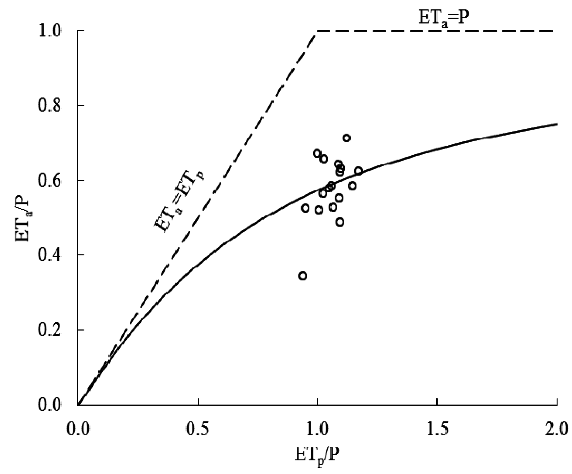
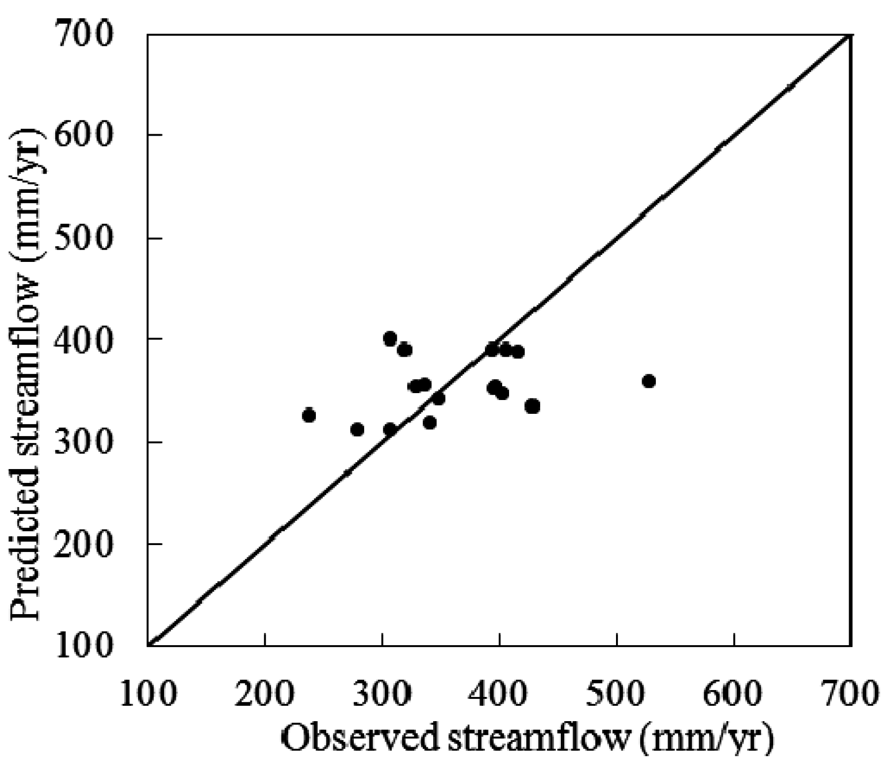
3.1. Mean Annual Water Balance in the Study Watersheds

The spatial variation in ET_p/P in the study watersheds was ranged from 0.94 to 1.17 (Table 1). This indicates that all the study watersheds are in a sub-humid climatic zone according to a study by Ponce et al. [37], in which the authors reported that climatic spectrum could be divided into eight types depending on ET_p/P ranges. Xu et al. [38] also reported similar ET_p/P ratios, which vary from 0.87 to 1.33 in 55 watersheds across the Midwest United States. Mean annual ET_a/P ratio and runoff coefficient (Q/P) in the study watersheds varied from 0.34 to 0.71 and from 0.29 to 0.66, respectively (Table 1). Low ET_a/P ratio under similar P was likely attributed to snowiness as Q in the Trap Rock River watershed mainly originated from snow fall and spring snowmelt [24]. Berghuijs et al. [39] also reported that snowy catchments have a high runoff ratio in context of the Budyko hypothesis. On average, 40% of long-term P in the study watersheds was converted into surface runoff. Mean annual Q/P ratios were large for watersheds with high BFI values, while the corresponding ET_a/P ratios were low. As shown in Figure 1, the relationship between mean annual ET_a/P and ET_p/P ratios in the study watersheds satisfied Fu’s curve with w = 1.95. Results indicated that estimated mean annual Q using Fu’s Equation (Equation (5)) agreed relatively well with observed mean annual Q with RMSE value of 64.1 mm/year (Figure 2).

Figure 1. Comparison of observed and calculated (using Fu’s Equation) ET_a/P in the study watersheds.

Figure 1. Comparison of observed and calculated (using Fu’s Equation) ET_a/P in the study watersheds.

Figure 2. Predicted vs. observed mean annual streamflow in the study watersheds.

Figure 2. Predicted vs. observed mean annual streamflow in the study watersheds.

3.2. Impact of Climatic Controls on Mean Annual Water Balance

Q sensitivity analysis indicated that mean annual Q increased from 12.6% in the Trap Rock River watershed to 20.6% in the Stony Creek watershed with an average value of 16.7% when mean annual P increased by 10% (Table 2). A 10% increase in ET_p decreased Q from 2.7% in the Trap Rock River watershed to 10.9% in the Stony Creek watershed with an average value of 6.9% (Table 2). Results also showed that streamflow sensitivity to changes in P and ET_p had a decreasing trend from north to south. Overall, mean annual Q was sensitive to variations in mean annual P and less sensitive to variations in mean annual ET_p for the period of 1967–2011 in all 17 watersheds. Similar results were found in a study conducted by Donohue et al. [40], in which the authors reported that Q increased by 7 mm/year with a 10 mm/year increase in P, and decreased by 4 mm/year for the same increase in ET_p in Australia for the period of 1981–2006. Roderick and Farquhar [8] applied this method in the semi-arid Murray Darling Basin in Australia and indicated that a 10% change in long-term average P yielded approximately 26% change in average Q. Herein, streamflow deviation ratio (SDR) (i.e., the ratio of the standard deviation of annual Q to that of annual P) proposed by Koster and Suarez [41] was used in this study to demonstrate the sensitivity of the variability in inter-annual Q to the variation in inter-annual P. Results indicated that SDR ranged from 0.35 in the Manistee River watershed to 1.05 in the Macatawa River watershed, suggesting that the majority of inter-annual P variability became inter-annual Q variability for the Macatawa River watershed, while inter-annual Q variability was largely less sensitive to variability in inter-annual P for the Manistee River watershed. SDR was low for watersheds with high BFI values, indicating that inter-annual Q variability was largely less sensitive to variability in inter-annual P for watersheds with high BFI values. It seemed that different contributions of baseflow to streamflow modified the impact of climate controls on water balance in the baseflow-dominated watersheds. That is to say, mean annual Q was less sensitive to climate change with the increase of BFI. Zeng and Cai [42] attributed ET variance to both the mean and variance of climatic variables by extending the framework of Koster and Suarez [41]. Results showed that catchment storage change played a significant role to buffer the inter- and intra-annual variance of ET in the Murray-Darling Basin.

Table 2. Sensitivity of mean annual Q to variations in mean annual P and ET_p in the study watersheds in Michigan.

Gaging Station ID	∂Q/∂P	∂Q/∂ETp	(P/Q) × (∂Q/∂P)	(ETp/Q) × (∂Q/∂ETp)
04040500	0.74	−0.29	1.57	−0.58
04043050	0.83	−0.19	1.26	−0.27
04045500	0.73	−0.26	1.53	−0.54
04057510	0.69	−0.26	1.64	−0.66
04059500	0.65	−0.27	1.80	−0.83
04096405	0.66	−0.31	1.92	−0.93
04105000	0.66	−0.26	1.75	−0.76
04105700	0.69	−0.26	1.66	−0.67
04108600	0.65	−0.33	2.00	−1.02
04108800	0.71	−0.27	1.62	−0.63
04117500	0.66	−0.26	1.77	−0.78
04122500	0.70	−0.24	1.56	−0.58
04124000	0.74	−0.21	1.44	−0.45
04127997	0.72	−0.24	1.52	−0.54
04161580	0.59	−0.28	2.06	−1.09
04164000	0.67	−0.23	1.62	−0.64
04166100	0.64	−0.23	1.70	−0.72

Table 2. Sensitivity of mean annual Q to variations in mean annual P and ET_p in the study watersheds in Michigan.

Gaging Station ID	∂Q/∂P	∂Q/∂ETp	(P/Q) × (∂Q/∂P)	(ETp/Q) × (∂Q/∂ETp)
04040500	0.74	−0.29	1.57	−0.58
04043050	0.83	−0.19	1.26	−0.27
04045500	0.73	−0.26	1.53	−0.54
04057510	0.69	−0.26	1.64	−0.66
04059500	0.65	−0.27	1.80	−0.83
04096405	0.66	−0.31	1.92	−0.93
04105000	0.66	−0.26	1.75	−0.76
04105700	0.69	−0.26	1.66	−0.67
04108600	0.65	−0.33	2.00	−1.02
04108800	0.71	−0.27	1.62	−0.63
04117500	0.66	−0.26	1.77	−0.78
04122500	0.70	−0.24	1.56	−0.58
04124000	0.74	−0.21	1.44	−0.45
04127997	0.72	−0.24	1.52	−0.54
04161580	0.59	−0.28	2.06	−1.09
04164000	0.67	−0.23	1.62	−0.64
04166100	0.64	−0.23	1.70	−0.72

4. Discussions

4.1. Compared with Other Similar Studies

All 17 study watersheds were located in a sub-humid climatic zone and thus climatic conditions of these watersheds were similar. However, ET_a/P ratios varied across the study watersheds. Previous studies suggested that differences in ET_a/P ratios under the same climatic aridity index were explained by land cover and/or soil texture [13,14,23]. Watersheds, such as Stony Creek watershed and Clinton River watershed had similar climate conditions (P and ET_p/P), with ET_a/P ratios of 0.71 and 0.59, respectively (Table 1). This may be due to the different percentages of soil types and land cover [43,44], with hydrologic soil group B comprising 73% and 57% of Stony Creek watershed and Clinton River watershed, respectively. Stony Creek watershed was mainly covered by forest (37%) while developed land cover constituted 65% of the Clinton River watershed. Overall, the varying ET_a/P ratios in the study watersheds could be the result of combinatory effects of land cover and soil properties. The average Q/P value of 0.42 during the 1967–2011 study period suggested that about 40% of long-term P in the study watersheds was converted into surface runoff. Similar results were found by Tekleab et al. [17], where Q/P ratios varied from 0.21 to 0.70 for 20 watersheds in the Upper Blue Nile basin. By contrast, Q/P ratios of 34 subbasins in the Nebraska Sand Hills reported by Wang et al. [23] were very low, ranging between 0.01 and 0.18, which can be explained by the high infiltration capacity of sandy soils in the Nebraska Sand Hills.

On average, 70% streamflow was contributed by baseflow in the studied watersheds [24]. As shown in Figure 3, the correlation coefficient between Q/P and BFI in the remaining 15 watersheds (Trap Rock River and Macatawa River watersheds were excluded) approaches to 0.5. It is suggested that Q/P ratios increased with the increase of BFIs. Similar results were reported by [23], which indicated that higher BFI values and Q/P ratio could be explained by higher groundwater recharge. Watersheds with similar BFI values would have similar ET_a/P ratios (e.g., Thornapple River and Battle Creek) (Table 1). Inversely, if BFI values were different, ET_a/P ratios would be different. Although average annual water balance was principally controlled by available water and energy (i.e., P and ET_p), factors such as rainfall seasonality, root zone storage capacity and snowiness have also been shown to be major controls on long-term water balance behavior [13,45]. Since Q/P ratio for the Trap Rock River and Macatawa River watersheds seemed unusual compared to the other study watersheds; they were not used for the analysis. As mentioned in Section 3.1., large Q in the Trap Rock River watershed could be the influence of heavy snow and large amounts of spring snowmelt. Low BFI values in the Macatawa River watershed could be explained by large proportions of agricultural and urban land uses as well as soil texture (dominated by hydrologic soil group C) that would reduce the rate of water transmission of the underlying aquifer and groundwater discharge into the streams [24]. Similar findings were reported in previous studies [8,23]. Wang et al. [23] indicated that soil texture altered the influence of climate on regional water balances to large extent and water storage should be included in the Budyko Hypothesis for baseflow-dominated watersheds.

Figure 3. Relationship between runoff coefficient (Q/P) and baseflow index (BFI).

Figure 3. Relationship between runoff coefficient (Q/P) and baseflow index (BFI).

4.2. Limitations

ET_p is an important variable for estimating ET_a and climate aridity index in hydrological modeling. Limited to the data availability, the Hargreaves method [30] was selected to calculate ET_p in this study. Since the Hargreaves equation was originally calibrated using data from California, the transferability of this equation to other regions is quite limited. The reliability of ET_p estimates can be improved by adding more relevant input variables [46,47]. Thus, the impact of ET_p calculated by Hargreaves method on mean annual water balance at watershed scales need to be further explored. Although Fu’s Equation was employed to estimate the role of climate changes on changing water balance conditions in this study, comparison of other empirical equations based on Budyko Hypothesis is necessary to be conducted in the future studies. In addition, watershed characteristics such as vegetation cover, soil properties and watershed topography were integrated in parameter w in Fu’s equation [15]; however, values of w in individual watersheds in this study were simply fitted between the observed ET_a/P and ET_p/P ratios. This may result in limitations in using Fu’s Equation for mean annual water balance estimation. Some studies have focused on the development of w estimation to improve the predictive ability of Fu’s Equation [45,48,49,50]. In addition, watershed boundaries were not considered in this study. This may result in water exchange within the adjacent watersheds, thereby limiting the accuracy of Fu’s Equation in estimating mean annual water balance in the study watersheds.

5. Conclusions

Mean annual water balances in 17 watersheds across Michigan were estimated using Fu’s equation, which is based on the Budyko Hypothesis. The role of climate controls (e.g., P and ET_p) on mean annual water balance was investigated with Fu’s Equation. Results indicated that estimated mean annual Q using Fu’s Equation agreed relatively well with observed mean annual Q with RMSE value of 64.1 mm/year. On average, 40% of long-term P in the study watersheds was converted into surface runoff. Mean annual Q/P ratios were large for watersheds with high BFI values, while the corresponding ET_a/P ratios were low, suggesting that Q was closely related to regional groundwater discharge. Climate sensitivity of mean annual Q showed that a 10% increase in mean annual P increased mean annual Q by 16.7%, while a 10% increase in mean annual ET_p decreased Q by 6.9% on average. This suggested that mean annual Q was sensitive to changes in mean annual P and less sensitive to changes in mean annual ET_p in all 17 watersheds. It seemed that different contributions of baseflow to streamflow modified the impact of climate controls on annual water balance in the baseflow-dominated watersheds.

References

1. Schreiber, P. Ueber die beziehungen zwischen dem niederschlag und der wasseruhrung der flusse in Mitteleuropa. Meteorol. Z. 1904, 21, 441–452. [Google Scholar]
2. Ol’dekop, E.M. On evaporation from the surface of river basins. Trans. Meteorol. Observ. 1911, 4, 200. [Google Scholar]
3. Budyko, M.I. The Heat Balance of the Earth’s Surface; US Department of Commerce: Washington, DC, USA, 1958. [Google Scholar]
4. Budyko, M.I. Climate and Life; Academic Press: San Diego, CA, USA, 1974; p. 508. [Google Scholar]
5. Choudhury, B.J. Evaluation of an empirical equation for annual evaporation using field observations and results from a biophysical model. J. Hydrol. 1999, 216, 99–110. [Google Scholar] [CrossRef]
6. Sankarasubramanian, A.; Vogel, R.M. Annual hydroclimatology of the United States. Water. Resour. Res. 2002, 38. [Google Scholar] [CrossRef]
7. Donohue, R.J.; Roderick, M.L.; McVicar, T.R. On the importance of including vegetation dynamics in Budyko’s hydrological model. Hydrol. Earth. Syst. Sci. 2007, 11, 983–995. [Google Scholar] [CrossRef]
8. Roderick, M.L.; Farquhar, G.D. A simple framework for relating variations in runoff to variations in climatic conditions and catchment properties. Water. Resour. Res. 2011, 47. [Google Scholar] [CrossRef]
9. Xiong, L.; Guo, S. Appraisal of Budyko formula in calculating long-term water balance in humid watersheds of southern China. Hydrol. Process. 2012, 26, 1370–1378. [Google Scholar] [CrossRef]
10. Turc, L. The water balance of soils. Relation between precipitation evaporation and flow. Ann. Agron. 1954, 5, 491–569. [Google Scholar]
11. Pike, J.G. The estimation of annual runoff from meteorological data in a tropical climate. J. Hydrol. 1964, 2, 116–123. [Google Scholar] [CrossRef]
12. Fu, B. On the calculation of the evaporation from land surface. Sci. Atmos. Sin. 1981, 5, 23–31. [Google Scholar]
13. Milly, P.C.D. Climate, soil water storage, and the average annual water balance. Water. Resour. Res. 1994, 30, 2143–2156. [Google Scholar] [CrossRef]
14. Zhang, L.; Dawes, W.R.; Walker, G.R. Response of mean annual evapotranspiration to vegetation changes at catchment scale. Water. Resour. Res. 2001, 37, 701–708. [Google Scholar] [CrossRef]
15. Zhang, L.; Hickel, K.; Dawes, W.R. A rational function approach for estimating mean annual Evapotranspiration. Water. Resour. Res. 2004, 40. [Google Scholar] [CrossRef]
16. Potter, N.J.; Zhang, L. Interannual variability of catchment water balance in Australia. J. Hydrol. 2009, 369, 120–129. [Google Scholar] [CrossRef]
17. Tekleab, S.; Uhlenbrook, S.; Mohamed, Y.; Savenije, H.H.G.; Temesgen, M.; Wenninger, J. Water balance modeling of Upper Blue Nile catchments using a top-down approach. Hydrol. Earth. Syst. Sci. 2011, 15, 2179–2193. [Google Scholar] [CrossRef]
18. Zhang, L.; Potter, N.; Hickel, K.; Zhang, Y.; Shao, Q. Water balance modeling over variable time scales based on the Budyko framework-Model development and testing. J. Hydrol. 2008, 360, 117–131. [Google Scholar]
19. Wang, H.; Yu, X. Sensitivity analysis of climate on streamflow in north China. Theor. Appl. Climatol. 2015, 119, 391–399. [Google Scholar] [CrossRef]
20. Liu, X.; Liu, W.; Xia, J. Comparison of the streamflow sensitivity to aridity index between the Danjiangkou Reservoir basin and Miyun Reservoir basin, China. Theor. Appl. Climatol. 2013, 111, 683–691. [Google Scholar] [CrossRef]
21. Wang, D.; Hejazi, M. Quantifying the relative contribution of the climate and direct human impacts on mean annual streamflow in the contiguous United States. Water. Resour. Res. 2011, 47, W00J12. [Google Scholar] [CrossRef]
22. Teng, J.; Chiew, F.H.S.; Vaze, J. Estimation of climate change impact on mean annual runoff across continental Australia using Budyko and Fu equations and hydrological models. J. Hydrometeorol. 2012, 13, 1094–1106. [Google Scholar] [CrossRef]
23. Wang, T.; Istanbulluoglu, J.L.; Scott, D. On the role of groundwater and soil texture in the regional water balance: An investigation of the Nebraska Sand Hills, USA. Water. Resour. Res. 2009, 45. [Google Scholar] [CrossRef]
24. Zhang, Y.; Ahiablame, L.; Engel, B.; Liu, J. Regression modeling of baseflow and baseflow index for Michigan USA. Water 2013, 5, 1797–1815. [Google Scholar] [CrossRef]
25. Daly, C.; Neilson, R.P.; Philips, D.L. A statistical-topographic model for mapping climatological precipitation over mountainous terrain. J. Appl. Meteorol. 1994, 33, 140–158. [Google Scholar] [CrossRef]
26. ArcGIS 10, Environmental Systems Resource Institute, Inc: Redlands, CA, USA, 2010.
27. USGS Current Water Data for the Nation. Available online: http://waterdata.usgs.gov/usa/nwis/rt (accessed on 10 November 2012).
28. Eckhardt, K. How to construct recursive digital filters for baseflow separation. Hydrol. Process. 2005, 19, 507–515. [Google Scholar] [CrossRef]
29. Lim, K.J.; Engel, B.A.; Tang, Z.; Chou, J.; Kim, K.S.; Muthukrishnan, S.; Tripathy, D. Automated web GIS-based hydrograph analysis tool, WHAT. J. Am. Water. Resour. Assoc. 2005, 41, 1407–1416. [Google Scholar] [CrossRef]
30. Hargreaves, G.H; Samani, Z.A. Reference crop evapotranspiration from temperature. Appl. Eng. Agric. 1985, 1, 96–99. [Google Scholar] [CrossRef]
31. Sankarasubramanian, A.; Vogel, R.M.; Limbrunner, J.F. Climate elasticity of streamflow in the United States. Water. Resour. Res. 2001, 37, 1771–1781. [Google Scholar] [CrossRef]
32. Hargreaves, G.H.; Allen, R.G. History and evaluation of Hargreaves evapotranspiration equation. J. Irrig. Drain. Eng. 2003, 129, 53–63. [Google Scholar] [CrossRef]
33. Bachour, R.; Walker, W.R.; Torres-Rua, A.F.; McKee, M. Assessment of reference evapotranspiration by the Hargreaves method in the Bekaa Valley, Lebanon. J. Irrig. Drain. Eng. 2013, 139, 933–938. [Google Scholar] [CrossRef]
34. Calculation of extraterrestrial solar radiation (to horizontal surface at top of atmosphere). Available online: http://www.engr.scu.edu/~emaurer/tools/calc_solar_cgi.pl (accessed on 20 April 2014).
35. Yang, D.; Sun, F.; Liu, Z.; Cong, Z.; Lei, Z. Interpreting the complementary relationship in non-humid environments based on the Budyko and Penman hypotheses. Geophys. Res. Lett. 2006, 33. [Google Scholar] [CrossRef]
36. Wang, D.; Alimohammadi, N. Responses of annual runoff, evaporation, and storage change to climate variability at the watershed scale. Water. Resour. Res. 2012, 48. [Google Scholar] [CrossRef]
37. Ponce, V.M.; Pandey, R.P.; Ercan, S. Characterization of drought across the climate spectrum. J. Hydrol. Eng. 2000, 5, 222–224. [Google Scholar] [CrossRef]
38. Xu, X.; Scanlon, B.R.; Schilling, K.; Sun, A. Relative importance of climate and land surface changes on hydrologic changes in the US Midwest since the 1930s: Implications for biofuel production. J. Hydrol. 2013, 497, 110–120. [Google Scholar] [CrossRef]
39. Berghuijs, W.R.; Woods, R.A.; Hrachowitz, M. A precipitation shift from snow towards rain leads to a decrease in streamflow. Nat. Clim. Chang. 2014, 4, 583–586. [Google Scholar] [CrossRef]
40. Donohue, R.J.; Roderick, M.L.; McVicar, T.R. Assessing the differences in sensitivities of runoff to changes in climatic conditions across a large basin. J. Hydrol. 2011, 406, 234–244. [Google Scholar] [CrossRef]
41. Koster, R.D.; Suarez, M.J. A simple framework for examining the interannual variability of land surface moisture fluxes. J. Clim. 1999, 12, 1911–1917. [Google Scholar] [CrossRef]
42. Zeng, R.; Cai, X. Assessing the temporal variance of evapotranspiration considering climate and catchment storage factors. Adv. Water. Resour. 2015, 79, 51–60. [Google Scholar] [CrossRef]
43. National Land Cover Data (NLCD). Available online: http://seamless.usgs.gov (accessed on 30 November 2012).
44. Soil Survey Geographic Database (SSURGO). Available online: http://soils.usda.gov/survey/geography (accessed on 8 January 2013).
45. Yang, D.; Sun, F.; Liu, Z.; Cong, Z.; Ni, G.; Lei, Z. Analyzing spatial and temporal variability of annual water-energy balance in nonhumid regions of China using the Budyko hypothesis. Water. Resour. Res. 2007, 43, W04426. [Google Scholar] [CrossRef]
46. Renner, M.; Bernhofer, C. Applying simple water-energy balance frameworks to predict the climate sensitivity of streamflow over the continental United States. Hydrol. Earth. Syst. Sci. 2012, 16, 2531–2546. [Google Scholar] [CrossRef]
47. Donohue, R.J.; McVicar, T.R.; Roderick, M.L. Assessing the ability of potential evaporation formulations to capture the dynamics in evaporative demand within a changing climate. J. Hydrol. 2010, 386, 186–197. [Google Scholar] [CrossRef]
48. Yang, D.; Shao, W.; Yeh, P.J.F.; Yang, H.; Kanae, S.; Oki, T. Impact of vegetation coverage on regional water balance in the nonhumid regions of China. Water. Resour. Res. 2009, 45. [Google Scholar] [CrossRef]
49. Donohue, R.J.; Roderick, M.L.; McVicar, T.R. Roots, storms and soil pores: Incorporating key ecohydrological processes into Budyko’s hydrological model. J. Hydrol. 2012, 436–437, 35–50. [Google Scholar] [CrossRef]
50. Xu, X.; Liu, W.; Scanlon, B.R.; Zhang, L.; Pan, M. Local and global factors controlling water-energy balances within the Budyko framework. Geophys. Res. Lett. 2013, 40, 6123–6129. [Google Scholar] [CrossRef]