Categorical Forecast of Precipitation Anomaly Using the Standardized Precipitation Index SPI

Abstract

In the paper, the verification of forecasts of precipitation conditions measured by the standardized precipitation index (SPI) is presented. For the verification of categorical forecasts, a contingency table was used. Standard verification measures were used for the SPI value forecast. The 30-day SPI, moved every 10 days by 10 days, was calculated in 2013–2015 from April to September on the basis of precipitation data from 35 meteorological stations in Poland. Predictions of the 30-day SPI were created in which precipitation was forecasted for the next 10 days (the SPI 10-day forecast) and 20 days (the SPI 20-day forecast). For both the 10 and 20 days, the forecasts were skewed towards drier categories at the expense of wet categories. There was a good agreement between observed and 10-day forecast categories of precipitation. Less agreement is obtained for 20-day forecasts—these forecasts evidently “over-dry” the assessment of precipitation anomalies. The 10-day SPI value forecast accuracy is very good or good depending on the performance measure, whereas accuracy of the 20-day forecast is unsatisfactory. Both for the SPI categorical and the SPI value forecast, the 10-day SPI forecast is trustworthy and the 20-day forecast should be accepted with reservation and used with caution.

1. Introduction

Modern economy uses natural—and at the same time highly weather-dependent—water resources. It needs trustworthy, good quality, short-, medium-, and long-term forecasts of surpluses and shortages of rainfall. In agriculture, knowledge of current rainfall and its forecast over the coming days enable the prediction of soil moisture changes, which allows farmers to take appropriate mitigation measures to reduce the negative effects of adverse weather events, mainly precipitation anomalies.

Natural and climatic conditions in Poland are generally conducive to agricultural production, but frequent changes of weather conditions during the growing season, especially rainfall, results in crop production periods of excessive soil moisture and, more often, deficient rainfall. Statistics show that the average loss in yields caused by drought ranged from 10% to 40%, and in extremely dry years (e.g., 1992 and 2000), meteorological drought covered more than 40% of Polish territory [1]. In Kujavian-Pomeranian province, losses caused by natural disasters in the years 1999–2011 totaled about 3.4 billion PLN [2]. Comparative research conducted by Bojar et al. [3] in Kujavian-Pomeranian (western Poland) and Lublin province (eastern Poland) showed significant differences in shortage of rainfall in agricultural production and yields of some crops due to regional differences in the precipitation amount and spatiotemporal distribution.

Forecasting rainfall, especially short- (1–2 days ahead) and medium-term (3–10 days ahead) is very important and significant in agriculture production. Monitoring and early warning help to reduce the impacts and to mitigate the consequences of weather- and climate-related natural disasters for agricultural production. Transfer of agrometeorological information to farmers can be done in different ways. Meteorological services use different options, such as periodical bulletins published on the Internet and mass media: TV, radio, and newspapers. According to Stigter et al. [4], the agrometeorological services should be simple so that they can be properly assimilated, and they must be used frequently to facilitate decision-making and planning. Agrometeorological services are often exemplified by agroclimatological characterization, weather forecasting (including agrometeorological forecasting), and other advisories prepared for farmers. Agrometeorological forecasting, with special attention to rainfall, is indispensable for planning agrotechnical measures such as plowing, sowing, and harvesting, not to mention irrigation, when rainfall amount is the main determinant of when and how much to irrigate.

Forecasting rainfall is one of the most difficult meteorological forecasts and has become one of the most important elements of forecasting weather conditions at various time scales. Powerful forecasting models have been used increasingly in recent years [5,6,7,8,9,10,11]. The results of forecasting are available on numerous web portals—of which the majority presents their own interpretations of graphic copyright forecasts published by specialized research institutes, such as the European Centre for Medium-Range Weather Forecasts [12] or the National Oceanic and Atmospheric Administration [10]—and by thematic weather portals, for example, Agropogoda [13] and WetterOnline [14]. For planning management of water in agriculture, medium- and long-term forecasts of rainfall are more valuable than the prediction of daily precipitation. However, the latter is important in operational control of irrigation.

Beside rainfall forecasts providing information of whether rainfall will occur and about the amount of rainfall in the forecast period, a categorical precipitation forecast is often made. Such a forecast informs on the category (class) that precipitation will be, either at a given probability or as a deterministic phenomenon. Moreover, for operational purposes and for making comparative assessments of precipitation anomalies in different regions, it is indispensable to apply not only precipitation data, but standardized precipitation data. One such index is the standardized precipitation index (SPI) [15,16]. The SPI has been defined as a key indicator for monitoring drought by the World Meteorological Organization [17]. The SPI is a standardized deviation of precipitation, in a particular period, from the median long-term value for this period. It represents a departure from the mean, expressed in standard deviation units. The SPI is a normalized index in time and space. The method ensures independence from geographical positions, as the index in question is calculated with respect to average precipitation in the same place [18].

An important issue in the forecasting process is the assessment of forecast accuracy. The results of verification of forecasts is the answer the question of whether the discrepancy between observed and forecast precipitation or precipitation category is essential according to accepted criteria. In world literature, there is a variety of assessment methods for the verification of predictive models, including the practice recommended by the World Meteorological Organization [19]. An interesting compendium of knowledge on forecasting is a collective work “Forecast Verification. A Practitioner’s Guide in Atmospheric Science” [20]. In that book, Livezey [21] discusses the assessment of conformity of the deterministic categorical forecasts with the actual situation according to the accepted multistage verification criteria.

There are rather few studies devoted to the assessment of forecast of drought identified by SPI. Bordi et al. [22] used two methods for forecasting the 1-month SPI: an autoregressive model (AR) and the Gamma Highest Probability (GAHP) method. The mean squared error (MSE) was relatively high for both methods. Mishra and Desai [23] used linear stochastic models—autoregressive integrated moving average (ARIMA) and multiplicative ARIMA (SARIMA) models—to forecast droughts using a series of SPI values in the Kangsabati River basin in India. Cancelliere et al. [24] proposed methods for forecasting transition probabilities from one drought class to another and for forecasting SPI. They showed that the SPI can be forecasted with a reasonable degree of accuracy, using conditional expectations based on past values of monthly precipitation. Hwang and Carbone [25] used a conditional resampling technique to generate ensemble forecasts of SPI, and found a reasonable forecast performance for SPI-1. Hannaford et al. [26] proposed a method for forecasting drought in the United Kingdom based on the current occurrence of drought. Shirmohammadi et al. [27] carried out research to evaluate the ability of wavelet artificial neural network (ANN) and adaptive neuro-fuzzy inference system (ANFIS) techniques for forecasting meteorological drought, as identified by SPI, in the southeastern part of East Azerbaijan province, Iran. The performances of the models were evaluated by comparing the corresponding values of the root mean squared error, the coefficient of determination, and the Nash–Sutcliffe model efficiency coefficient. Belayneh et al. [28] compared the effectiveness of five data-driven models for forecasting long-term (6- and 12-month lead-time) drought conditions in the Awash River Basin of Ethiopia. The standard precipitation index was forecasted using a traditional stochastic model (ARIMA) and compared to machine learning techniques such as ANNs and support vector regression (SVR). The performances of all models were compared using the root mean squared error (RMSE), the mean absolute error (MAE), the coefficient of determination (R²), and a measure of persistence. Maca and Pech [29] compared forecast of drought indices based on two different models of artificial neural networks. The analyzed drought indices were the SPI and the standardized precipitation evaporation index (SPEI), which were derived for the period of 1948–2002 on two U.S. catchments. The comparison of the models was based on six model performance measures.

Most of the methods used to forecast SPI are based purely on statistics. There are much fewer reports in the literature of an assessment of SPI forecast based on numerical prediction models of precipitation. Łabędzki and Bąk [30] conducted a verification of the 10-day forecasts of rainfall and the course of meteorological drought in 2009 and 2010 for the station of the Institute of Technology and Life Sciences (ITP) in Bydgoszcz (Poland). The authors checked the validity of the forecasts of precipitation taken from the service WetterOnline and the forecasts of rainfall categories based on SPI using their own verification criteria. Singleton [31] analyzed the performance of the European Centre for Medium Range Weather Forecasts (ECMWF) variable resolution ensemble prediction system (varEPS) for predicting the probability of meteorological drought. Drought intensity was measured by the SPI, and forecasts of SPI-1 and SPI-3 were verified against independent observations.

Since April 2013, the Institute of Technology and Life Sciences (ITP) has been conducting nationwide monitoring and forecasting of shortage and excess of water in Poland [32]. The current assessment of precipitation anomalies and earlier 20- and 10-day forecasts are based on actual and projected values of the standardized precipitation index, SPI. The spatial distribution of deficit and excess rainfall are shown on the maps in real-time and forecast periods. They are available on the website of the Institute of Technology and Life Sciences (www.itp.edu.pl)—Monitoring Agrometeo (http://agrometeo.itp.edu.pl).

The aim of the study is to evaluate the verifiability of these rainfall category forecasts predicted in 2013–2015.

2. Materials and Methods

2.1. SPI Calculation and Precipitation Categories

The evaluation and forecasting of precipitation anomalies (rainfall deficit and surplus) are made using the standardized precipitation index, SPI. The SPI calculation for any location is based on the long-term precipitation record in a given period. SPI was calculated using the normalization method. Precipitation P is a random variable with a lower limit and often positive asymmetry and does not conform to normal distribution. Most often, periodical (monthly, half-year, or annual) sums of precipitation conform to the gamma distribution. Therefore, precipitation sequence was normalized with the transformation function f(P):

$$f\left(P\right)=u=\sqrt[3]{P}$$

(1)

where P is the element of precipitation sequence.

Values of the SPI for a given P are calculated with the equation:

$$SPI=\frac{f\left(P\right)-\overline{u}}{d_u}$$

(2)

where SPI is the standardized precipitation index, f(P) is the transformed sum of precipitation, $\overline{u}$ is the mean value of the normalized precipitation sequence, and d_u is the standard deviation of the normalized precipitation sequence.

The values of SPI are compared with the boundaries of different classes. Because the SPI is normalized, wet and dry periods can be classified symmetrically. There are many classifications used by different authors. Originally, McKee et al. [15] distinguished four classes of drought and four classes of wet periods: mild, moderate, severe, and extreme. The threshold value of SPI for the mild drought and mild wet category equals to SPI = 0. Agnew [33] writes that, in this classification, all negative values of SPI are taken to indicate the occurrence of drought—this means that for 50% of the time drought is occurring. He concluded that it was not rational and suggested alternative, more rational thresholds. He recommended the SPI drought thresholds corresponding to 20% (moderate drought), 10% (severe drought), and 5% (extreme drought) probabilities (SPI = −0.84, −1.28 and −1.65, respectively). Vermes [34] proposed seven categories, with the first class of a dry period starting at SPI = −1 and with the wet period at SPI = 1. In this study, this classification was applied (

Table 1. Precipitation categories according to SPI.

Category	SPI
Extremely dry	≤−2.0
Very dry	−2.0 < SPI ≤ −1.5
Moderately dry	−1.5 < SPI ≤ −1.0
Normal	−1.0 < SPI ≤ 1.0
Moderately wet	1.0 < SPI ≤ 1.5
Very wet	1.5 < SPI ≤ 2.0
Extremely wet	>2.0

).

2.2. Data Set

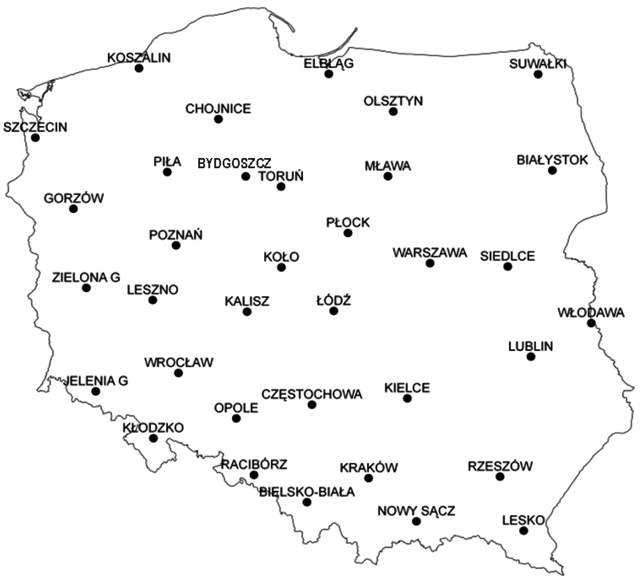
The SPI values are calculated on the basis of precipitation data from 35 meteorological stations of the Institute of Meteorology and Water Management (IMGW)—National Research Institute in Poland (Figure 1). Series of precipitation records from the period 1961–2012, at each station, were used as historical data.

The SPI was calculated in 2013–2015 from April to September and for the 30(31)-day periods moved every 10(11) days by 10(11) days (called “observed SPI”). Using the forecasted precipitation, predictions of the 30(31)-day SPI are created in which precipitation is forecasted in the next 10(11) (called “the SPI 10-day forecast”) and 20(21) days (called “the SPI 20-day forecast”). It means that, for example, when the observed SPI is in the period from 11 May to 10 June, the 10-day SPI forecast covers the period 21 May–20 June in which precipitation from 21 May to 10 June is observed and from 11 June to 20 June is forecasted. The 20-day SPI forecast covers the period from 1 June to 30 June, in which precipitation from 1 June to 10 June is observed and from 11 June to 20 June is forecasted. In the verification procedure, the pairs of the observed and forecast SPI in the same period are taken for comparison separately for the 10 and 20 day forecasts. Altogether, there were 1330 observed–forecasted pairs for each forecast type (10-day and 20-day)—10 periods in 2013, 14 periods in 2014 and 14 periods in 2015. The period of 10, 20, and 30 days refers to the calendar decade with 10, 20, and 30 days and the period of 11, 21, and 31 to the calendar decade with 11, 21, and 31 days. The observed and forecast SPI was calculated in 2013–2015 using Equations (1) and (2), in which $\overline{u}$ and d_u were determined for the 1961–2012 historical precipitation sequence. The historical precipitation data series from 1961 to 2012 (52 years) is indispensable and used for calculation of SPI in 2013–2015.

Rainfall forecasts necessary to develop predictions of precipitation anomalies for the next 10 and 20 days come from the meteorological service of MeteoGroup [9]. MeteoGroup has developed its own system of forecasting called multi-model MOS (model output statistics), which is based on numerical model calculations of the most respected meteorological centers—ECMWF model (European Centre for Medium-Range Weather Forecasts), EPS model (Ensemble Prediction System), GFS (Global Forecast System) model (National Centers for Environmental Prediction), UKMO model (United Kingdom Met Office)—as well as on the measurement and observation data from all available sources (national synoptic meteorological stations, aerodrome meteorological stations, satellite images, and radar images). The calculation results of each model are included with different weights. For each location, where historical measurements are available (with at least 1 year), for each meteorological element are assigned appropriate weights based on the degree of verifiability of each of the models in the past. Weighting is held every year with the new data. Major updates of MOS forecasts are held four times a day (7, 9, 19, and 21 UTC) based on the new model results (2–4 times a day depending on the model). In addition, MOS forecast is updated continuously as the inflow of the measurement data (1–3 h). Also, a special tool (Meteobase) is developed that, if necessary, allows meteorologists to enter manual adjustments to the forecasts at any time. MeteoGroup can provide forecast for any location specified by the user. For this purpose, the method of so-called “smart interpolation” is used, taking into account the results of the forecasts for the neighboring measuring stations, with weights dependent on their distance from the location and degree of similarity in terms of location (height above sea level, distance from the sea, location in a mountain valley, etc.). There is also the possibility of including measurement data supplied by the user, which further improves the quality of predictions for the location.

The forecasts, presented and analyzed in the paper, are deterministic forecasts of a nominal variable. The variable is the standardized precipitation index, SPI, whose value in a given period is qualified to the one of the SPI categories. The short-range forecast of SPI issued 10 days ahead and medium-range forecast covering the next 20 days were made.

2.3. Verification Procedure

Verification of two types of the SPI forecast was made: the SPI category forecast and the SPI value forecast.

For the verification of categorical forecasts, the distribution approach was used. This approach relies on the analysis of the joint distribution for forecasts and observations and examines the relationship among the elements in the multicategory contingency table, which is considered a good tool for this purpose [21,35]. A contingency table is a type of table in a matrix format that displays the multivariate frequency distribution of the variables. It provides a basic picture of the interrelation between two variables and can help find interactions between them.

A contingency table shows the distribution of one variable in rows and another in columns to study the association between the two variables. The two-way contingency table is a two-dimensional table that gives the discrete joint sample distribution of deterministic forecasts and categorical observations in cell counts [21]. The contingency table is a combination of two or more frequency tables arranged in such a way that each cell in the table clearly represents a combination of specific values of the analyzed variables. Such a multiway table enables the analysis of the frequencies corresponding to the categories designated by more than one variable. By analyzing these frequencies, you can identify the relationships that exist between the variables.

Each cell of the contingency table contains the relative frequency p_ij of forecast category i and observed category j. It is calculated as the cell count n_ij divided by the total forecast–observation pair sample size n. The sums of p_ij for a given forecast category i and observed category j are called marginal frequencies.

To test if frequencies in each category of observed and forecasted SPI values are strongly dependent (i.e., there is a significant relationship between them) the Pearson chi-squared test (χ²) was used. The null hypothesis is that they are not dependent (there is no relationship between them) and the contingency table is the result of independent forecast–observation pairs for categorical events. High statistical significance of the dependence of observed and forecasted SPI category indicates high forecast accuracy. The χ² test consists of comparing observed frequencies with expected frequencies with the assumption of the null hypothesis (no association between observed and predicted values). Expected frequency E_ij is calculated using the empirical marginal distributions as:

$$E_{ij}={\displaystyle \sum }_{j=1}^k{p}_{ij}{\displaystyle \sum }_{i=1}^k{p}_{ij} /{\displaystyle \sum }_{i=1}^k{\displaystyle \sum }_{j=1}^k{p}_{ij} i, j=1, \dots , k$$

(3)

where:

• p_ij—relative frequency of forecast category i and observed category j
• k—number of observed and forecast categories

The test statistic, called the Pearson chi-squared statistic, takes the form:

$${\mathsf{\chi }}^2={\displaystyle \sum }_{i=1}^k{\displaystyle \sum }_{j=1}^k\frac{{\left(p_{ij}-E_{ij}\right)}^2}{E_{ij}}$$

(4)

Assuming the veracity of the null hypothesis, this statistic has the asymptotic χ² distribution with the degrees of freedom df equal to:

$$df={\left(k-1\right)}^2$$

(5)

The results of observed–forecast frequencies depend on the relation of the number of categories and the sample size. For more than two categories forecast, a sample size required for proper estimates should be of the order of 10k² [21]. In the presented study, k = 7 and the sample size of 1330 forecast–observation pairs is thus completely sufficient.

If the values of the computed statistic according to Equation (4) exceed the critical χ²_cr for their chance probabilities to be less than e.g., 0.05, 0.01, 0.001 (χ² > χ²_cr) the null hypothesis can be rejected at a given probability level. The asymptotic distribution of χ² for different degrees of freedom is tabulated in different sources from which χ²_cr can be determined for a given probability and the sample size n.

For categorical forecasts presented in the form of a contingency table, the following measures of accuracy were used based on the frequencies and the marginal distributions:

(1)

Proportion correct PC

$$PC={\displaystyle \sum }_{i=1}^k{p}_{ii}$$

(6)

(2)

Bias B

$$B_i={\displaystyle \sum }_{j=1}^k{p}_{ij}/{\displaystyle \sum }_{j=1}^k{p}_{ji} i=1, \dots , k$$

(7)

(3)

Probability of detection POD

$$PO{D}_i=p_{ii}/{\displaystyle \sum }_{j=1}^k{p}_{ji} i=1, \dots , k$$

(8)

(4)

Heidke skill score HSS

$$HSS=\left({\displaystyle \sum }_{i=1}^k{p}_{ii}-{\displaystyle \sum }_{i=1}^k{p}_i{\overline{p}}_i\right)/\left(1-{\displaystyle \sum }_{i=1}^k{p}_i{\overline{p}}_i\right)$$

(9)

in which

$$p_i={\displaystyle \sum }_{j=1}^k{p}_{ji} i=1, \dots , k$$

(10)

$${\overline{p}}_i={\displaystyle \sum }_{j=1}^k{p}_{ij} i=1, \dots , k$$

(11)

Besides the verification of the SPI category forecasts on the basis of the contingency table, the verifiability of the SPI value forecasts was assessed. The following measures of goodness of fit were used to evaluate the forecast performance:

(1)

Ratio of the number of the periods in which the criterion

$$\left|SP{I}_{forecast}-SP{I}_{observed}\right|\le 0.5$$

(12)

was met to the number of all periods.

(2)

Mean systematic error (bias) b

$$b=\frac{1}{n}{\displaystyle \sum }_{i=1}^n\left(SP{I}_{forecast}-SP{I}_{observed}\right)$$

(13)

where n is the number of forecast–observation pairs.

(3)

Mean absolute error MAE

$$MAE=\frac{1}{n}{\displaystyle \sum }_{i=1}^n\left|SP{I}_{forecast}-SP{I}_{observed}\right|$$

(14)

(4)

Root mean squared error RMSE

$$RMSE=\sqrt{\frac{1}{n}{\displaystyle \sum }_{i=1}^n{\left(SP{I}_{forecast}-SP{I}_{observed}\right)}^2}$$

(15)

(5)

Pearson’s linear correlation coefficient r

$$r=\frac{{\displaystyle {\sum }_{i=1}^n\left(SP{I}_{forecast}-{\overline{SPI}}_{forecast}\right)\left(SP{I}_{observed}-{\overline{SPI}}_{observed}\right)}}{\sqrt{{\displaystyle {\sum }_{i=1}^n{\left(SP{I}_{forecast}-{\overline{SPI}}_{forecast}\right)}^2}}\sqrt{{\displaystyle {\sum }_{i=1}^n{\left(SP{I}_{observed}-{\overline{SPI}}_{observed}\right)}^2}}}$$

(16)

In the above equations, SPI_forecast denotes the forecast SPI value in the 30(31)-day period in which the 20(21)-day rainfall sum was measured and the 10(11)-day rainfall sum was forecast in the case of the 10-day forecast, and the 10(11)-day rainfall sum was measured and the 20(21)-day rainfall was forecast in the case of the 20-day forecast. SPI_observed denotes the observed SPI value in the same 30(31)-day period on the basis of the measured rainfall sum in this period.

3. Results and Discussion

3.1. SPI Category Forecast

The joint distribution of forecast and observed SPI is presented in the contingency tables for the 10-day forecasts (

Table 2. Relative frequency (in percent) for the standardized precipitation index (SPI) 10-day forecasts (n = 1330).

Forecast	Observed
	Extremely Dry	Very Dry	Moderately Dry	Normal	Moderately Wet	Very Wet	Extremely Wet	Forecast Distribution
Extremely dry	3	1	1	1	0	0	0	6
Very dry	1	3	3	1	0	0	0	8
Moderately dry	1	2	5	5	0	0	0	13
Normal	0	0	3	56	3	1	0	63
Moderately wet	0	0	0	2	3	1	0	6
Very wet	0	0	0	1	1	1	0	3
Extremely wet	0	0	0	0	0	0	1	1
Observed distribution	5	6	12	66	7	3	1	100

Notes: n—the number of observation–forecast pairs.

) and for the 20-day forecasts (

Table 3. Relative frequency (in percent) for SPI 20-day forecasts (n = 1330).

Forecast	Observed
	Extremely Dry	Very Dry	Moderately Dry	Normal	Moderately Wet	Very Wet	Extremely Wet	Forecast Distribution
Extremely dry	3	2	3	4	0	0	0	12
Very dry	1	2	2	7	0	0	0	12
Moderately dry	1	1	3	11	0	0	0	16
Normal	0	1	4	42	6	1	1	55
Moderately wet	0	0	0	2	1	1	0	4
Very wet	0	0	0	0	0	1	0	1
Extremely wet	0	0	0	0	0	0	0	0
Observed distribution	5	6	12	66	7	3	1	100

). The contingency tables show the relative frequencies and the empirical margins distributions in seven categories of precipitation. The forecasts were made for 35 stations and for the years 2013–2015 for April through September. Each table is constructed from a sample of 1330 forecasts–observations.

Based on the distribution of the observed SPI, it can be concluded that in 2013–2015, the periods drier than normal dominated (23%) in comparison with the wetter periods (11%). Normal periods occurred most often (66%). A similar frequency distribution was found for the forecasts, both for 10 and 20 days ahead. These forecasts are skewed towards forecasts of drier categories at the expense of wet categories—27% of the periods were predicted to be drier than normal in the case of 10-day forecasts and 30% in the case of 20-day forecasts. Comparing the distribution of observations and forecasts, it seems reasonable to conclude that there is a good agreement between observed and 10-day forecast categories of precipitation. Less agreement is obtained for 20-day forecasts—these forecasts evidently “over-dry” the assessment of precipitation anomalies. The observed normal category of precipitation is almost as often as the 10-day forecast of this category (66% and 63%, respectively). The 20-day forecast of normal category is less frequent (55%) than the observed normal category. The frequency of 20-day forecast of dry periods distinctly increased, while that of normal and wet periods decreased.

To answer the question of whether the constructed contingency tables are the result of dependent forecast–observations pairs for categorical events, a chi-squared test (χ²) was performed with the assumption of the null hypothesis that no association between observed and predicted values occurred. For the 10-day forecast, the test statistics χ² are greater than the critical values χ²_cr at the 0.05, 0.01, and 0.001 level (

Table 4. Chi-squared (χ²) values for SPI forecasts in seven categories (n = 1330; df = 36).

Test Statistic	10-Day Forecast	20-Day Forecast
χ2 calculated	155.7	51.5
χ2cr for α = 0.05	51.0
χ2cr for α = 0.01	58.6
χ2cr for α = 0.001	68.0

Notes: n—the number of observation-forecast pairs; df—degree of freedom.

). For the 20-day forecast the test statistic χ² is greater than the critical values χ²_cr at the 0.05 level. This means that the null hypothesis should be rejected at the 0.001 level for the 10-day forecast and at the 0.05 level for 20-day forecast. The relation between the frequency distribution in SPI categories is statistically significant at least at the 0.001 level for the 10-day forecast and at the 0.05 level for the 20-day forecast. A crucial point is whether these levels of statistical significance are satisfactory or not (i.e., at which level the results given in the contingency table are statistically significant). I proposed to assume the level of 0.001. Thus, the 10-day categorical forecasts of SPI are satisfactory and acceptable and the 20-day forecasts are not.

For categorical forecasts, the measures of accuracy based on the frequencies and the marginal distributions are shown in

Table 5. Measures of accuracy for SPI forecasts in seven categories.

Measure	Extremely Dry	Very Dry	Moderately Dry	Normal	Moderately Wet	Very Wet	Extremely Wet
	10-day forecast
PC	0.72
HSS	0.47
B	1.63	1.15	1.08	0.94	0.85	0.92	1.38
POD	0.64	0.52	0.46	0.83	0.42	0.42	0.69
	20-day forecast
PC	0.51
HSS	0.19
B	3.13	1.89	1.49	0.80	0.50	0.45	0.56
POD	0.67	0.28	0.27	0.62	0.13	0.18	0.19

Notes: PC—proportion correct; HSS—Heidke skill score; B—bias; POD—probability of detection.

.

The proportion of correct PC shows the proportion of correct categorical forecasts. PC is rather high for 10-day forecasts (72%) and lower for 20-day forecasts (51%).

The HSS measures the fractional improvement of the forecast over the standard forecast. It answers the question of what the accuracy of the forecast in predicting the correct category is, relative to that of random chance. It measures the fraction of correct forecasts after eliminating those forecasts which would be correct due purely to random chance. The range of the HSS is −∞ to 1. Negative values indicate that the chance forecast is better, 0 means no skill, and a perfect forecast obtains an HSS of 1. According to these criteria, the 10-day forecast may be evaluated as good and the 20-day forecast is not satisfactory due to HSS being close to 0.

The bias B reveals whether some forecast categories are over- or under-forecast. In the case of the 10-day forecasts, the forecast–observation set has little bias B for the normal as well as for the moderately and very dry and wet categories (value close to 1). The forecasts and observations are rather dissimilar for the extreme category. The values of bias B are worse for the 20-day forecasts. For both the 10-day and 20-day forecasts, the dry categories are above-forecast (B > 1) and the wet categories are under-forecast (B < 1).

The probability of detection POD quantifies the success rate for detecting different categorical events. The probability of detection is only satisfactory for the 10-day normal category forecast (POB = 0.83); other forecasts are modestly under-detected.

3.2. SPI Value Forecast

In this section, the verification of the SPI value forecast is presented (

Table 6. Measures of accuracy for SPI value forecasts.

Measure	10-Day Forecast	20-Day Forecast
Ratio	72%	40%
b	−0.10	−0.53
MAE	0.39	0.80
RMSE	0.543	1.037
Correlation coefficient r	0.870	0.648

Notes: MAE—mean absolute error; RMSE—root mean squared error; b—mean systematic error (bias).

).

Performance measures and corresponding performance evaluation criteria are important aspects of forecast verification. A forecast is high quality if it predicts the observed conditions well according to some objective or subjective criteria. A logical question to ask is about these criteria is which values of the above measures show that the forecasts are satisfactory and acceptable. The answer can be approached by comparing the obtained results with the thresholds. The problem is that there is no unique standard classification of these measures in relation to meteorological forecasts and, especially, the SPI forecasts. The forecasts are naturally more trustworthy when verification measures are as close as possible to the perfect score. There is a need to put some error bounds on the verification results. According to [35], the perfect score for bias b, MAE, and RMSE is 0 and for r is 1. The other approach is to refer the forecast errors to the standard deviation of the observed values or to determine confidence intervals for the verification measures. In this study, evaluation of the gained errors—referring them to the possible most often occurring SPI range and to the standard deviation—was performed. Using the criteria described by Moriasi et al. [36,37]—that RMSE may be regarded as low when it is less than 50% of the standard deviation of the observations—the forecast meeting this criterion is treated as being very good. When the ratio of RMSE to the standard deviation is between 0.5 and 0.6, the forecast is good; between 0.6 and 0.7—satisfactory; and when greater than 0.7—unsatisfactory. The same criterion is used in relation to MAE in this study.

The first measure of the accuracy—the ratio of the number of the periods in which the absolute value of the difference between the forecast and observed SPI was not greater than 0.5 of the number of all periods—averaged for all stations, was 72% for the 10-day forecast and 40% for the 20-day forecast. At different stations, the ratio changes from 54% to 85% for the 10-day forecast and from 18% to 58% for the 20-day forecast.

The mean systematic error (bias) is negative (−0.10 for 10-day forecast and −0.53 for 20-day forecast). This means that the forecasts are too dry on average. This verification measure in not fully adequate because negative errors can be compensated by positive errors. The mean absolute error MAE avoids this disadvantage since it takes into the account absolute values of the individual forecast error. The MAE is used to measure how close forecasted values are to the observed values. It is the average of the absolute errors. Results show that the positive and negative errors of the SPI forecast are twice greater for the 20-day forecast than for the 10-day forecast. However, the MAE of 10-day forecast (0.39) is relative small—10% compared to the range of the most often observed SPI values (from −2 to 2) and is 38% compared to the standard deviation of the observed SPI equal to 1.03.

The root-mean-squared error (RMSE) is the square root of the mean squared error of the forecast, which measures the average of the squares of the errors, which is the difference between the forecast and observed SPI. RMSE is the square root of the second moment of the error, and thus incorporates both the variance of the forecast and its bias. The value RMSE = 0.54 for the 10-day forecast seems to be acceptable, taking into account the possible range of SPI and its ratio to the standard deviation. This ratio is equal to 52% and it qualifies the 10-day forecast as good, according to the criteria proposed by Moriasi et al. [36,37]; the 20-day forecast is unsatisfactory (RMSE > 1).

The last measure most often used for evaluation of the forecasts is simply the correlation coefficient r between forecast and observed values. This coefficient measures the degree of association among the forecast and observed values. It is satisfactory for 10-day forecast (0.87) and unsatisfactory for 20-day forecast (0.65).

Those low values of bias b, MAE, and RMSE and the high value of r for the 10-day forecast indicate that the predicted estimates are close to the measured values.

Belayneh et al. [28] validated different models of forecasting SPI by comparing the errors and, on this basis, showing which is model is better. For SPI-6 and SPI-12, they obtained MAE = 0.20 ÷ 0.39, RMSE = 0.32 ÷ 0.90, and r = 0.72 ÷ 0.96 for different models and stations. These values are comparable with the values obtained for the 10-day forecast in this study. Unfortunately, these authors do not refer the errors to any classification. Maca and Pech [29], analyzing the forecast of SPI using two types of neural network models, found similar MAE and RMSE values. The performances of the different wavelet models for forecasting meteorological drought—identified by SPI in southeastern part of East Azerbaijan province, Iran—were evaluated by comparing RMSE and R² [27]. The best performance measures were obtained for the wavelet ANFIS model predicting SPI one, two, and three months ahead—RMSE was about 0.1 and R² = 0.90 ÷ 0.98. They are a little better than the results obtained in this study.

Comparison of the results presented in this paper with the results found in the other studies warrants the statement that forecasting the 30-day SPI with the 10-day precipitation forecast is burdened with similar errors as those obtained when forecasting SPI with other methods, mainly neutral network and wavelet analysis. The performance measures were used mostly to compare different models and to indicate the model or the method which gave the better indicators. Unfortunately, there is no guidance on how to classify the received errors and measures. Further work should be focused on the development of the objective evaluation standards and classification of the SPI forecast performance.

4. Conclusions

This study investigated the accuracy of forecasts of precipitation conditions measured by the standardized precipitation index, SPI. Verification of two types of the SPI forecast was performed: the SPI category forecast and the SPI value forecast. For the verification of categorical forecasts, a contingency table was used. Standard verification measures were used for the SPI value forecast. The SPI was calculated for the 30(31)-day periods, moved every 10(11) days by 10(11) days. Using the forecasted precipitation, predictions of the 30(31)-day SPI were created in which precipitation was forecasted for the next 10(11) and 20(21) days.

In 2013–2015, for both the 10 and 20 days, the forecasts were skewed towards forecasts of drier categories at the expense of wet categories. Comparing the distribution of observations and forecasts, there was a good agreement between observed and 10-day forecast categories of precipitation. Less agreement is obtained for 20-day forecasts—these forecasts evidently “over-dry” the assessment of precipitation anomalies. The observed normal category of precipitation was almost as often as the 10-day forecast of this category. The 20-day forecast of normal category was less frequent than the observed normal category. The frequency of 20-day forecast of dry periods distinctly increased, while that of normal and wet periods decreased. The Heidke skill score shows that the 10-day forecast may be evaluated as good and the 20-day forecast is not satisfactory. Considering the SPI values, the ratio of the number of the periods in which the absolute value of the difference between the forecasted and observed SPI was not greater than 0.5 to the number of all periods, averaged for all stations, was 72% for the 10-day forecast and 40% for the 20-day forecast. Considering the measures of the SPI value forecast accuracy, the accuracy of the 20-day forecast was shown to be weaker than of the 10-day forecast. The mean absolute error MAE of the SPI forecast was twice greater for the 20-day forecast than for the 10-day forecast. The MAE of the 10-day forecast was relatively small compared to the range of the most often observed SPI values and the standard deviation of the observed values. It indicates that this forecast as very good. Other measures (the square root of mean squared error RMSE, the correlation coefficient) also shows that the 10-day forecast accuracy is good, whereas for the 20-day forecast is unsatisfactory.

The performed analysis shows that, both for the SPI categorical and the SPI value forecast, the 10-day SPI forecast is trustworthy and the 20-day forecast should be accepted with reservation and used with caution. Whatever the case, the SPI forecasts should be viewed critically, especially in an operational mode, as it is made in the system of monitoring and forecasting water deficit and surplus conducted in Poland by ITP (http://agrometeo.itp.edu.pl).