
Including Condition into Ecological Maps Changes Everything—A Study of Ecological Condition in the Conterminous United States

 ,
,  , and
, and 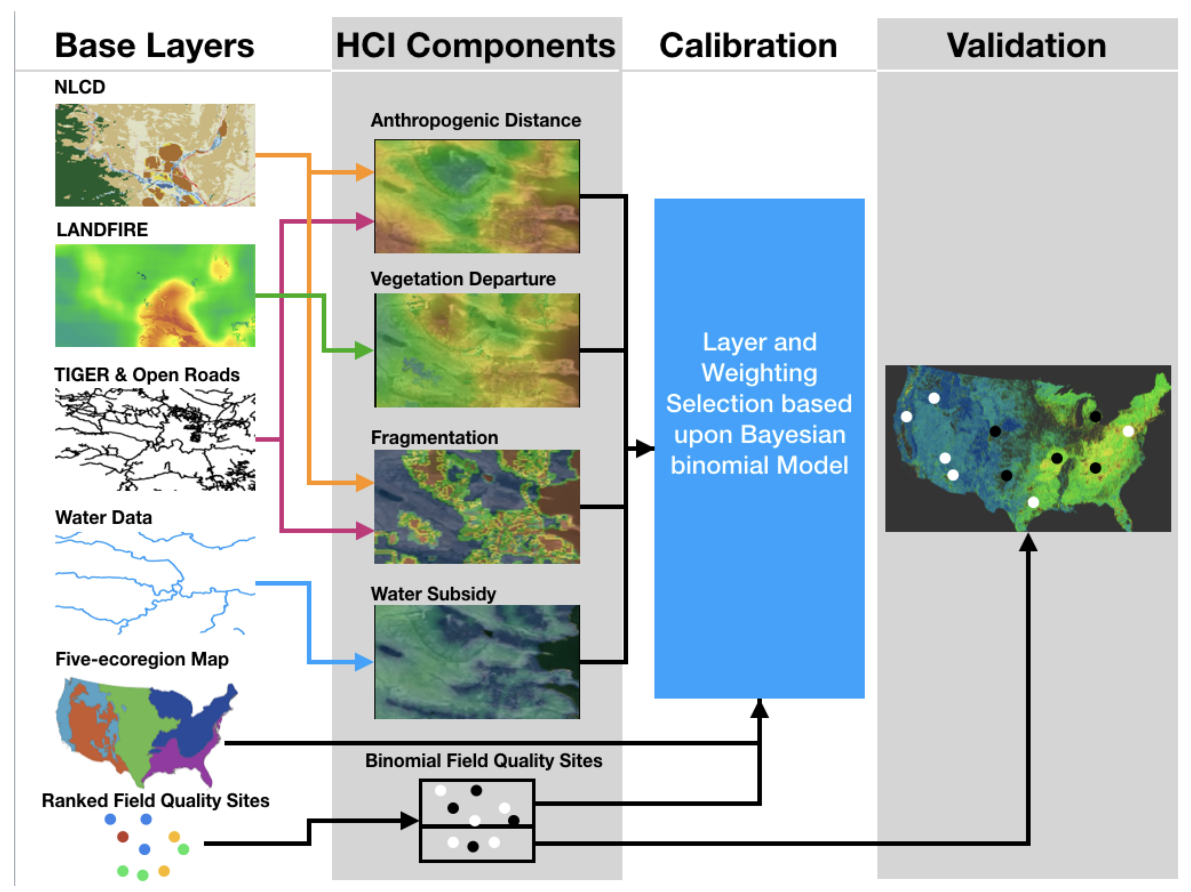
Abstract
:1. Introduction
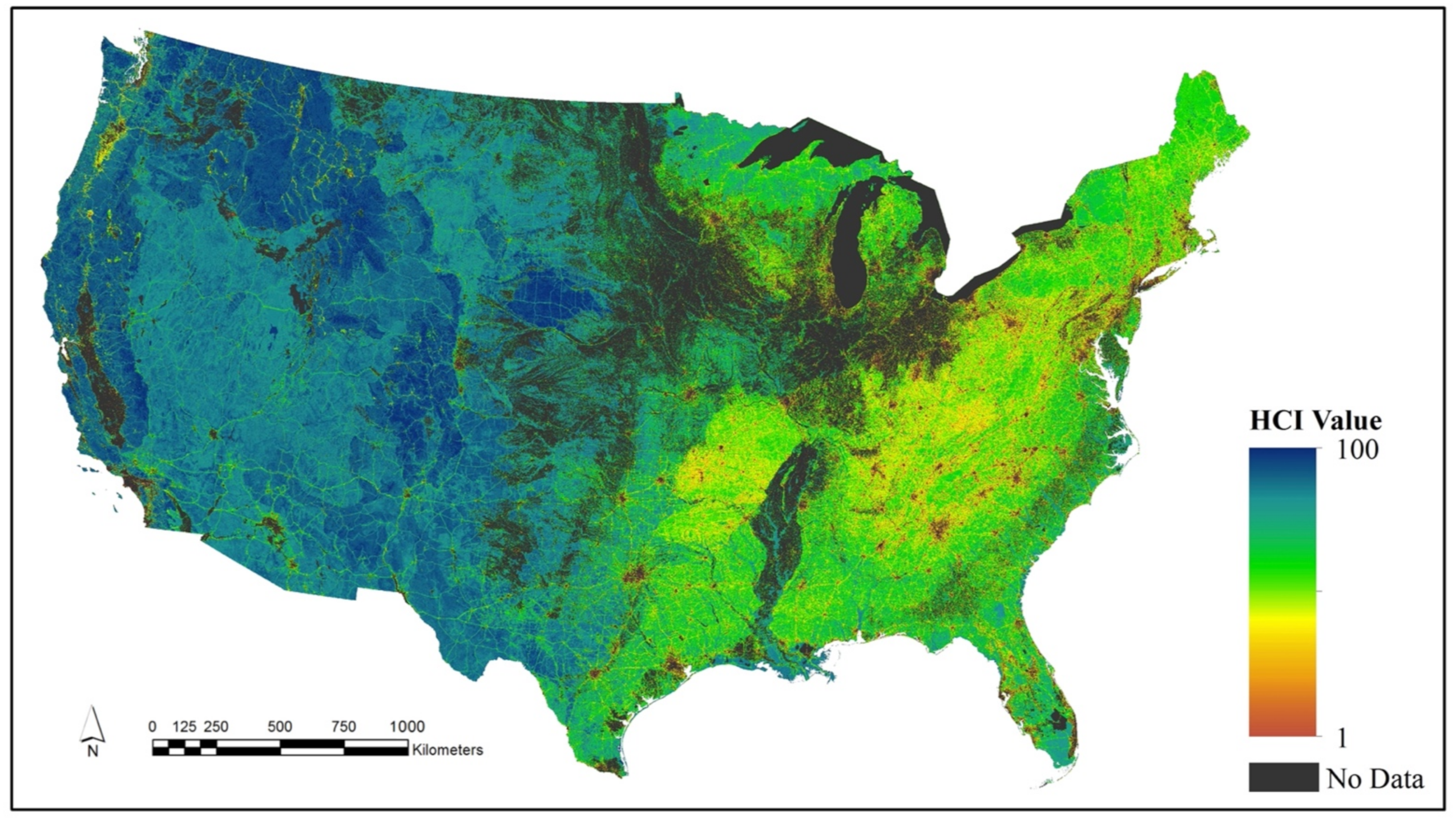
- Areal estimates of habitat area significantly overestimate the capacity of land to support biodiversity, because they may assume the quality of natural habitat areas is pristine (or 100% quality which is a 100 HCI score). By measuring ‘functional’ area of habitat (i.e., area × HCI value), the HCI values more accurately represent the relative capacity of the land to support healthy, thriving ecosystems and the species they support when compared to a hypothetical “pristine” landscape. Thus, comparing areal estimates of habitat with HCI scores on those same lands tests the degree of degradation of the natural landscape across the CONUS.
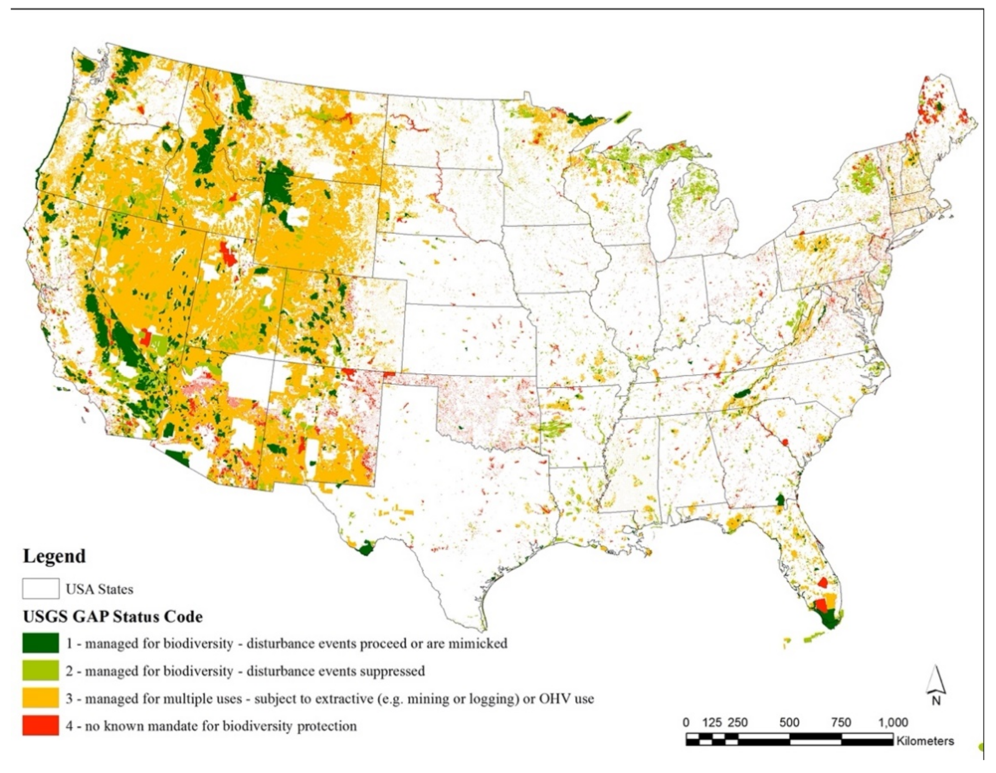
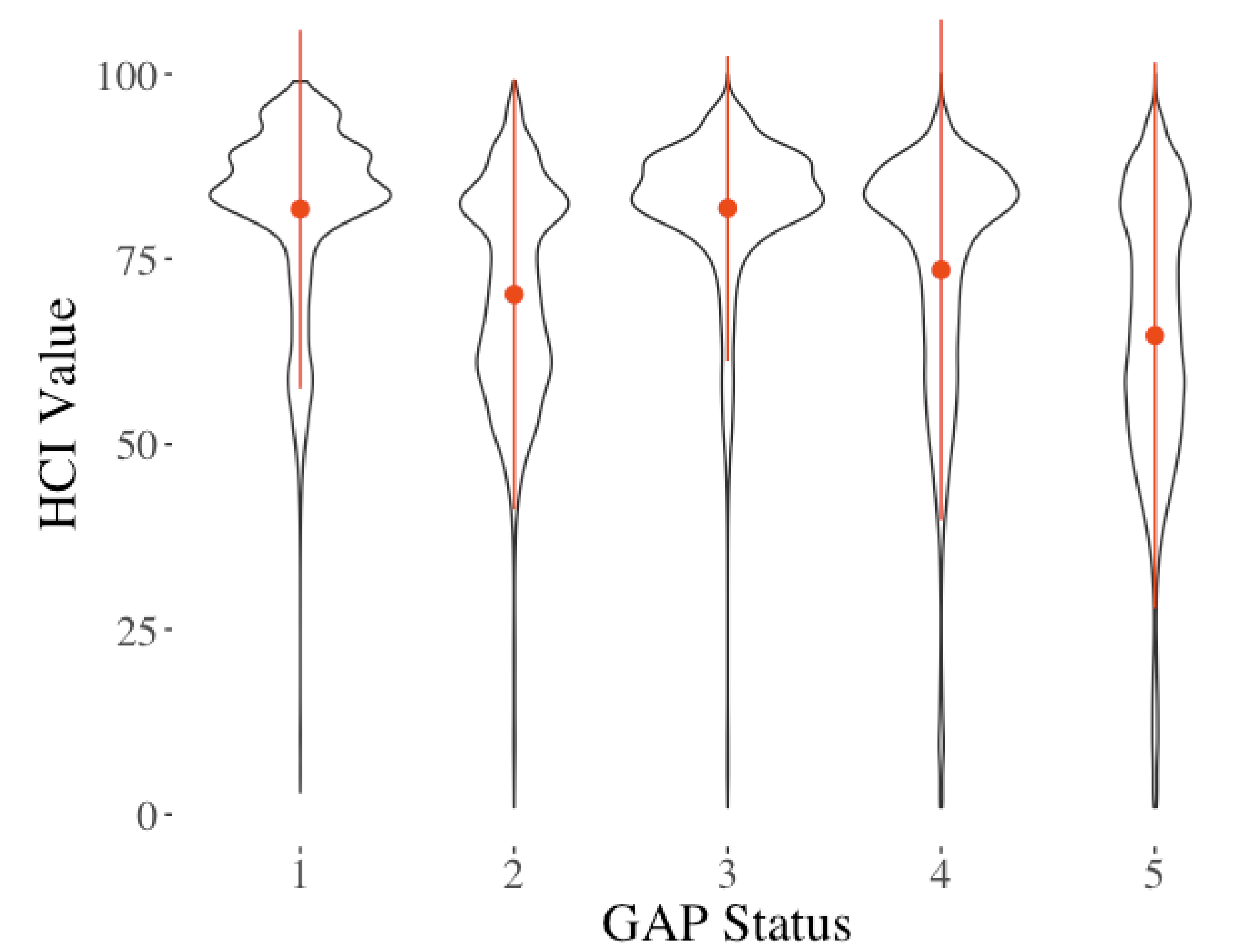
- Lands designated for biodiversity conservation alone will have higher average landscape condition (HCI values) than lands designated for multiple use. This hypothesis examines the differences between various levels of conservation status as indicators of the effectiveness of land protection policies.
- HCI values of natural and semi-natural lands do not correlate with ownership (public versus privately owned). This hypothesis tests whether management influences habitat quality.
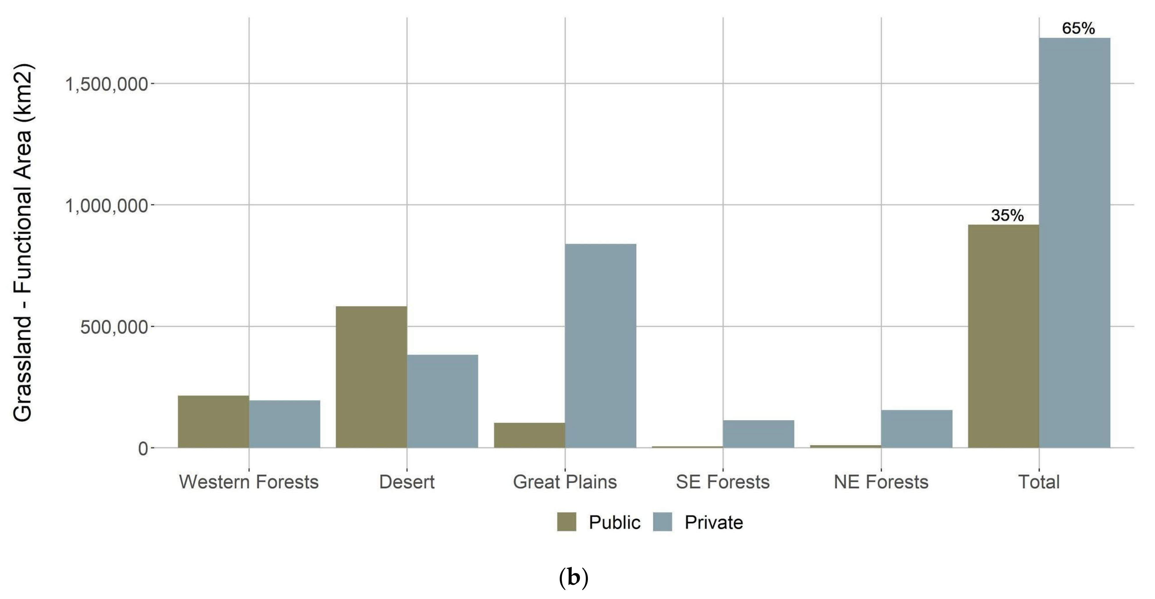
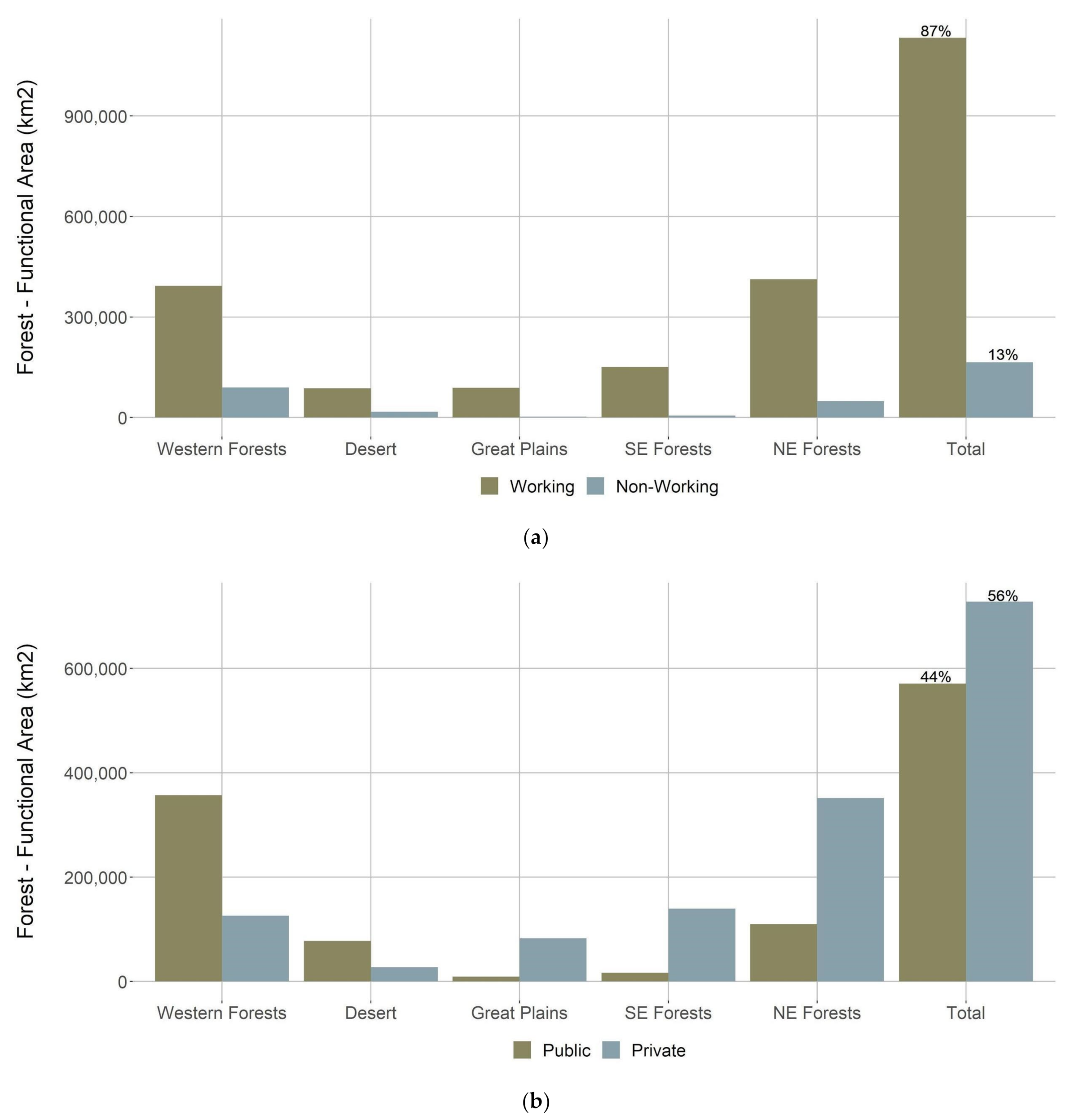
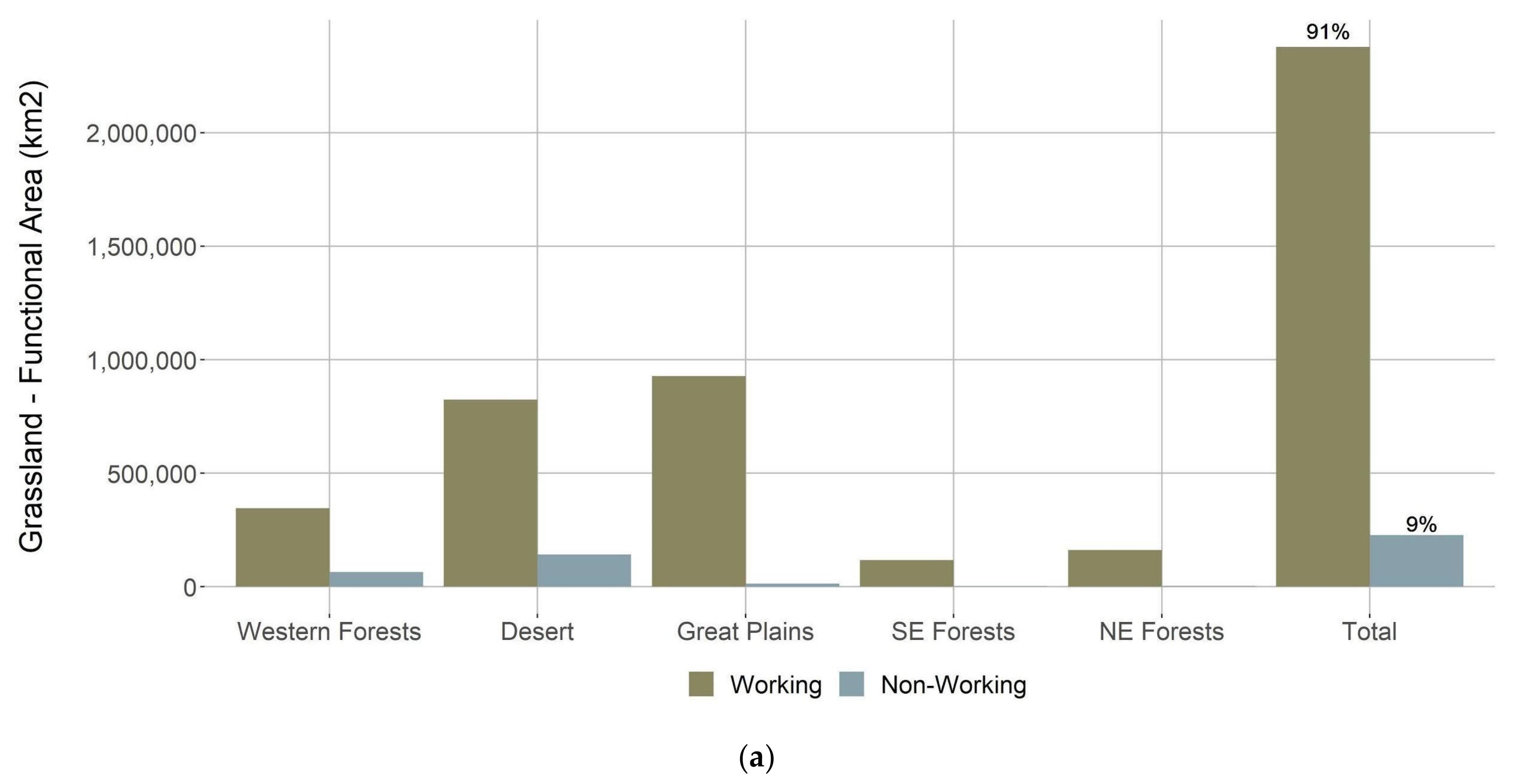
- Privately-owned natural and semi-natural working lands (i.e., lands in range or silvicultural production), regardless of management or use, comprise a large percentage of total functional habitat of the CONUS. This hypothesis tests the assumption that privately-owned lands may be critical for wildlife conservation if public lands are not sufficiently large or of high enough quality [53,54,55,56,57].
- The sum of HCI-weighted values for currently protected and unprotected lands in the CONUS are greater than that needed to conserve 30% of the U.S. This hypothesis tests whether the 30 by 30 goal is theoretically possible.
2. Materials and Methods
2.1. Base Data Layer Selection and Spatial Analysis
2.1.1. Habitat Fragmentation
2.1.2. Anthropogenic Influence
2.1.3. Vegetation Departure from Pre-European Conditions
2.1.4. Proximity to Aquatic Resources
2.2. Calibration
2.3. Creation of the HCI
2.4. Validation
2.5. Hypothesis Testing
3. Results
Hypothesis Results
4. Discussion
5. Conclusions
Supplementary Materials
Author Contributions
Funding
Acknowledgments
Conflicts of Interest
References
- Biden, J. Executive Order on Tackling the Climate Crisis at Home and Abroad. 2021. Available online: https://www.whitehouse.gov/briefing-room/presidential-actions/2021/01/27/executive-order-on-tackling-the-climate-crisis-at-home-and-abroad/ (accessed on 3 March 2021).
- Prior-Magee, J.S.; Johnson, L.J.; Croft, M.J.; Case, M.L.; Belyea, C.M.; Voge, M.L. Protected Areas Database of the United States (PAD-US) 2.1; USGS: Reston, VI, USA, 2020. [Google Scholar]
- Ferraro, P.J.; McIntosh, C.; Ospina, M. The Effectiveness of the US Endangered Species Act: An Econometric Analysis Using Matching Methods. J. Environ. Econ. Manag. 2007, 54, 245–261. [Google Scholar] [CrossRef]
- Burns, C.E.; Johnston, K.M.; Schmitz, O.J. Global Climate Change and Mammalian Species Diversity in U.S. National Parks. Proc. Natl. Acad. Sci. USA 2003, 100, 11474–11477. [Google Scholar] [CrossRef] [PubMed] [Green Version]
- Woodley, S.; Kay, J. Ecological Integrity and the Management of Ecosystems; CRC Press: Boca Raton, FL, USA, 1993; ISBN 978-0-9634030-1-8. [Google Scholar]
- Halvorson, W.L.; Davis, G.E. Science and Ecosystem Management in the National Parks; University of Arizona Press: Tucson, AZ, USA, 1996; ISBN 978-0-8165-1566-0. [Google Scholar]
- Monz, C.; D’Antonio, A.; Lawson, S.; Barber, J.; Newman, P. The Ecological Implications of Visitor Transportation in Parks and Protected Areas: Examples from Research in US National Parks. J. Transp. Geogr. 2016, 51, 27–35. [Google Scholar] [CrossRef]
- Bowman, J.; Forbes, G.; Dilworth, T. Landscape Context and Small-Mammal Abundance in a Managed Forest. For. Ecol. Manag. 2001, 140, 249–255. [Google Scholar] [CrossRef]
- Questad, E.J.; Foster, B.L.; Jog, S.; Kindscher, K.; Loring, H. Evaluating Patterns of Biodiversity in Managed Grasslands Using Spatial Turnover Metrics. Biol. Conserv. 2011, 144, 1050–1058. [Google Scholar] [CrossRef]
- Butler, S.J.; Vickery, J.A.; Norris, K. Farmland Biodiversity and the Footprint of Agriculture. Science 2007, 315, 381–384. [Google Scholar] [CrossRef]
- Briske, D.D.; Bestelmeyer, B.T.; Brown, J.R.; Brunson, M.W.; Thurow, T.L.; Tanaka, J.A. Assessment of USDA-NRCS Rangeland Conservation Programs: Recommendation for an Evidence-Based Conservation Platform. Ecol. Appl. 2017, 27, 94–104. [Google Scholar] [CrossRef] [Green Version]
- Oetting, J.B.; Knight, A.L.; Knight, G.R. Systematic Reserve Design as a Dynamic Process: F-TRAC and the Florida Forever Program. Biol. Conserv. 2006, 128, 37–46. [Google Scholar] [CrossRef]
- Rittenhouse, C. Conservation Planning: Informed Decisions for a Healthier Planet. Landsc. Ecol. 2017, 32, 2219–2221. [Google Scholar] [CrossRef]
- Comer, P.J.; Hak, J.C.; Josse, C.; Smyth, R. Long-Term Loss in Extent and Current Protection of Terrestrial Ecosystem Diversity in the Temperate and Tropical Americas. PLoS ONE 2020, 15, e0234960. [Google Scholar] [CrossRef]
- Bracy Knight, K.; Seddon, E.S.; Toombs, T.P. A Framework for Evaluating Biodiversity Mitigation Metrics. Ambio 2020, 49, 1232–1240. [Google Scholar] [CrossRef] [PubMed]
- Pimentel, D.; Westra, L.; Noss, R.F. (Eds.) Ecological Integrity: Integrating Environment, Conservation, and Health, 1st ed.; Island Press: Washington, DC, USA, 2000; ISBN 978-1-55963-807-4. [Google Scholar]
- Unnasch, R.S.; Braun, D.P.; Comer, P.J.; Eckert, G.E. The Ecological Integrity Assessment Framework; Springer: Berlin/Heidelberg, Germany, 2019. [Google Scholar]
- Keith, D.A.; Rodríguez, J.P.; Rodríguez-Clark, K.M.; Nicholson, E.; Aapala, K.; Alonso, A.; Asmussen, M.; Bachman, S.; Basset, A.; Barrow, E.G.; et al. Scientific Foundations for an IUCN Red List of Ecosystems. PLoS ONE 2013, 8, e62111. [Google Scholar] [CrossRef] [PubMed] [Green Version]
- Bull, J.W.; Suttle, K.B.; Gordon, A.; Singh, N.J.; Milner-Gulland, E.J. Biodiversity Offsets in Theory and Practice. Oryx 2013, 47, 369–380. [Google Scholar] [CrossRef] [Green Version]
- Chiavacci, S.J.; Pindilli, E.J. Trends in Biodiversity and Habitat Quantification Tools Used for Market-based Conservation in the United States. Conserv. Biol. 2020, 34, 125–136. [Google Scholar] [CrossRef] [Green Version]
- Fennessy, M.S.; Stein, E.D.; Ambrose, R.; Craft, C.B.; Herlihy, A.T.; Kentula, M.E.; Kihslinger, R.; Mack, J.J.; Novitski, R.; Banker, M.; et al. Towards a National Evaluation of Compensatory Mitigation Sites: A Proposed Study Methodology; Environmental Law Institute: Washington, DC, USA, 2013; p. 27. [Google Scholar]
- Fennessy, M.S.; Jacobs, A.D.; Kentula, M.E. Review of Rapid Methods for Assessing Wetlands Condition; National Health and Environmental: Corvallis, OR, USA, 2004. [Google Scholar]
- Carreras Gamarra, M.J.; Toombs, T.P. Thirty Years of Species Conservation Banking in the U.S.: Comparing Policy to Practice. Biol. Conserv. 2017, 214, 6–12. [Google Scholar] [CrossRef]
- Swaty, R.; Blankenship, K.; Hagen, S.; Fargione, J.; Smith, J.; Patton, J. Accounting for Ecosystem Alteration Doubles Estimates of Conservation Risk in the Conterminous United States. PLoS ONE 2011, 6, e23002. [Google Scholar] [CrossRef] [PubMed] [Green Version]
- Leu, M.; Hanser, S.; Knick, S. The Human Footprint in the West: A Large-Scale Analysis of Anthropogenic Impacts. Ecol. Appl. A Publ. Ecol. Soc. Am. 2008, 18, 1119–1139. [Google Scholar] [CrossRef] [PubMed]
- Bennett, A.F.; Saunders, D.A. Habitat fragmentation and landscape change. In Conservation Biology for All; Sodhi, N.S., Ehrlich, P.R., Eds.; Oxford University Press: Oxford, UK, 2010; pp. 88–106. ISBN 978-0-19-955423-2. [Google Scholar]
- Sanderson, E.W.; Jaiteh, M.; Levy, M.A.; Redford, K.H.; Wannebo, A.V.; Woolmer, G. The Human Footprint and the Last of the Wild: The Human Footprint Is a Global Map of Human Influence on the Land Surface, Which Suggests That Human Beings Are Stewards of Nature, Whether We like It or Not. BioScience 2002, 52, 891–904. [Google Scholar] [CrossRef]
- Bayne, E.M.; Hobson, K.A. The Effects of Habitat Fragmentation by Forestry and Agriculture on the Abundance of Small Mammals in the Southern Boreal Mixedwood Forest. Can. J. Zool. 1998, 76, 10. [Google Scholar] [CrossRef]
- Aguilar, R.; Ashworth, L.; Galetto, L.; Aizen, M.A. Plant Reproductive Susceptibility to Habitat Fragmentation: Review and Synthesis through a Meta-Analysis. Ecol Lett. 2006, 9, 968–980. [Google Scholar] [CrossRef] [PubMed]
- Haddad, N.M.; Brudvig, L.A.; Clobert, J.; Davies, K.F.; Gonzalez, A.; Holt, R.D.; Lovejoy, T.E.; Sexton, J.O.; Austin, M.P.; Collins, C.D.; et al. Habitat Fragmentation and Its Lasting Impact on Earth’s Ecosystems. Sci. Adv. 2015, 1, e1500052. [Google Scholar] [CrossRef] [PubMed] [Green Version]
- Koehler, G.M.; Maletzke, B.T. Habitat Fragmentation and the Persistence of Lynx Populations in Washington State. J. Wildl. Manag. 2008, 7, 1518–1524. [Google Scholar]
- Schmiegelo, F.A. Habitat Loss and Fragmentation in Dynamic Landscapes: Avian Perspectives from the Boreal Forest. Ecol. Appl. 2002, 16, 375–389. [Google Scholar]
- Collingham, Y.C.; Huntley, B. Impacts of Habitat Fragmentation and Patch Size Upon Migration Rates. Ecol. Appl. 2000, 10, 131–144. [Google Scholar] [CrossRef]
- Gehring, T.M.; Swihart, R.K. Body Size, Niche Breadth, and Ecologically Scaled Responses to Habitat Fragmentation: Mammalian Predators in an Agricultural Landscape. Biol. Conserv. 2003, 109, 283–295. [Google Scholar] [CrossRef]
- Andrén, H.; Angelstam, P.; Lindström, E.; Widén, P. Differences in Predation Pressure in Relation to Habitat Fragmentation: An Experiment. Oikos 1985, 45, 273–277. [Google Scholar] [CrossRef]
- Hoffmeister, T.S.; Vet, L.E.M.; Biere, A.; Holsinger, K.; Filser, J. Ecological and Evolutionary Consequences of Biological Invasion and Habitat Fragmentation. Ecosystems 2005, 8, 657–667. [Google Scholar] [CrossRef]
- El Araby, M. Urban Growth and Environmental Degradation. Cities 2002, 19, 389–400. [Google Scholar] [CrossRef]
- Previtali, M.A.; Lehmer, E.M.; Pearce-Duvet, J.M.C.; Jones, J.D.; Clay, C.A.; Wood, B.A.; Ely, P.W.; Laverty, S.M.; Dearing, M.D. Roles of Human Disturbance, Precipitation, and a Pathogen on the Survival and Reproductive Probabilities of Deer Mice. Ecology 2010, 91, 582–592. [Google Scholar] [CrossRef]
- Bradley, C.A.; Altizer, S. Urbanization and the Ecology of Wildlife Diseases. Trends Ecol. Evol. 2007, 22, 95–102. [Google Scholar] [CrossRef] [PubMed]
- Riitters, K.H.; Wickham, J.D.; O’Neill, R.V.; Jones, K.B.; Smith, E.R.; Coulston, J.W.; Wade, T.G.; Smith, J.H. Fragmentation of Continental United States Forests. Ecosystems 2002, 5, 815–822. [Google Scholar] [CrossRef]
- Angermeier, P.L.; Karr, J.R. Biological Integrity Versus Biological Diversity as Policy Directives: Protecting Biotic Resources. In Ecosystem Management: Selected Readings; Samson, F.B., Knopf, F.L., Eds.; Springer: New York, NY, USA, 1996; pp. 264–275. ISBN 978-1-4612-4018-1. [Google Scholar]
- Parrish, J.D.; Braun, D.P.; Unnasch, R.S. Are We Conserving What We Say We Are? Measuring Ecological Integrity within Protected Areas. BioScience 2003, 53, 851. [Google Scholar] [CrossRef] [Green Version]
- Theobald, D.M. A General Model to Quantify Ecological Integrity for Landscape Assessments and US Application. Landsc. Ecol. 2013, 28, 1859–1874. [Google Scholar] [CrossRef]
- Hak, J.C.; Comer, P.J. Modeling Landscape Condition for Biodiversity Assessment—Application in Temperate North America. Ecol. Indic. 2017, 82, 206–216. [Google Scholar] [CrossRef]
- Miller, C. The Hidden Consequences of Fire Suppression. Park Sci. 2012, 28, 75–80. [Google Scholar]
- Block, W.M.; Conner, L.M.; Brewer, P.A.; Ford, P.; Haufler, J.; Litt, A.; Masters, R.E.; Mitchell, L.R.; Park, J. Effects of Prescribed Fire on Wildlife and Wildlife Habitat in Selected Ecosystems of North America; The Wildlife Society: Bethesda, MD, USA, 2016; p. 681. [Google Scholar]
- Brooks, M.L.; D’Antonio, C.M.; Richardson, D.M.; Grace, J.B.; Keeley, J.E.; DiTomaso, J.M.; Hobbs, R.J.; Pellant, M.; Pyke, D. Effects of Invasive Alien Plants on Fire Regimes. BioScience 2004, 54, 677. [Google Scholar] [CrossRef] [Green Version]
- Netusil, N.R. Economic Valuation of Riparian Corridors and Upland Wildlife Habitat in an Urban Watershed: Economic Valuation of Riparian Corridors. J. Contemp. Water Res. Educ. 2009, 134, 39–45. [Google Scholar] [CrossRef] [Green Version]
- Johnson, D. Habitat Fragmentation Effects on Birds in Grasslands and Wetlands: A Critique of Our Knowledge. Great Plains Res. 2001, 11, 22. [Google Scholar]
- Polis, G.; Power, M.; Huxel, G. Food Webs at the Landscape Level. Bibliovault Oai Repos. Univ. Chic. Press 2004, 1, 523. [Google Scholar]
- Baxter, C.V.; Fausch, K.D.; Carl Saunders, W. Tangled Webs: Reciprocal Flows of Invertebrate Prey Link Streams and Riparian Zones: Prey Subsidies Link Stream and Riparian Food Webs. Freshw. Biol. 2005, 50, 201–220. [Google Scholar] [CrossRef]
- Muehlbauer, J.D.; Collins, S.F.; Doyle, M.W.; Tockner, K. How Wide Is a Stream? Spatial Extent of the Potential “Stream Signature” in Terrestrial Food Webs Using Meta-Analysis. Ecology 2014, 95, 44–55. [Google Scholar] [CrossRef] [PubMed]
- Murphy, D.D.; Noon, B.R. The Role of Scientists in Conservation Planning on Private Lands. Conserv. Biol. 2007, 21, 25–28. [Google Scholar] [CrossRef]
- Norton, D.A. Conservation Biology and Private Land: Shifting the Focus. Conserv. Biol. 2000, 14, 1221–1223. [Google Scholar] [CrossRef]
- Paloniemi, R.; Tikka, P.M. Ecological and Social Aspects of Biodiversity Conservation on Private Lands. Environ. Sci. Policy 2008, 11, 336–346. [Google Scholar] [CrossRef]
- Macaulay, L. The Role of Wildlife-Associated Recreation in Private Land Use and Conservation: Providing the Missing Baseline. Land Use Policy 2016, 58, 218–233. [Google Scholar] [CrossRef] [Green Version]
- Cortés Capano, G.; Toivonen, T.; Soutullo, A.; Di Minin, E. The Emergence of Private Land Conservation in Scientific Literature: A Review. Biol. Conserv. 2019, 237, 191–199. [Google Scholar] [CrossRef]
- Homer, C.; Dewitz, J.; Jin, S.; Xian, G.; Costello, C.; Danielson, P.; Gass, L.; Funk, M.; Wickham, J.; Stehman, S.; et al. Conterminous United States Land Cover Change Patterns 2001–2016 from the 2016 National Land Cover Database. Isprs. J. Photogramm. Remote Sens. 2020, 162, 184–199. [Google Scholar] [CrossRef]
- Vogt, P. GuidosToolbox: Universal Digital Image Object Analysis. Eur. J. Remote. Sens. 2017, 50, 352–361. [Google Scholar] [CrossRef]
- Vogt, P.; Riitters, K.H.; Estreguil, C.; Kozak, J.; Wade, T.G.; Wickham, J.D. Mapping Spatial Patterns with Morphological Image Processing. Landsc. Ecol. 2007, 22, 171–177. [Google Scholar] [CrossRef]
- Landfire Vegetation Departure Dataset; USGS: Reston, VA, USA, 2017.
- Pratt, S.; Holsinger, L.; Keane, R.E. Chapter 10—Using simulation modeling to assess historical reference conditions for vegetation and fire regimes for the LANDFIRE prototype project. Rollins, M.G., Frame, C.K., Eds.; In The LANDFIRE Prototype Project: Nationally Consistent and Locally Relevant Geospatial Data for Wildland Fire Management Gen. Tech. Rep. RMRS-GTR-175; U.S. Department of Agriculture, Forest Service, Rocky Mountain Research Station: Fort Collins, CO, USA, 2006; Volume 175, pp. 277–314. [Google Scholar]
- Rollins, M.G. LANDFIRE: A Nationally Consistent Vegetation, Wildland Fire, and Fuel Assessment. Int. J. Wildland Fire 2009, 18, 235. [Google Scholar] [CrossRef] [Green Version]
- NatureServe. Element Occurrence Data Standard 2002. Available online: http://downloads.natureserve.org/conservation_tools/element_occurence_data_standard.pdf (accessed on 2 February 2020).
- Vehtari, A.; Gelman, A.; Gabry, J. Practical Bayesian Model Evaluation Using Leave-One-out Cross-Validation and WAIC. Stat. Comput. 2017, 27, 1413–1432. [Google Scholar] [CrossRef] [Green Version]
- Yao, Y.; Vehtari, A.; Simpson, D.; Gelman, A. Using Stacking to Average Bayesian Predictive Distributions (with Discussion). Bayesian Anal. 2018, 13, 917–1007. [Google Scholar] [CrossRef]
- Thompson, J.R.; Carpenter, D.N.; Cogbill, C.V.; Foster, D.R. Four Centuries of Change in Northeastern United States Forests. PLoS ONE 2013, 8, e72540. [Google Scholar] [CrossRef] [PubMed] [Green Version]
- Riitters, K.H. Spatial Patterns of Land Cover in the United States: A Technical Document Supporting the Forest Service 2010 RPA Assessment; Department of Agriculture Forest Service, Southern Research Station: Asheville, NC, USA, 2011; p. 64. [Google Scholar]
- Thomas, B.F. Sustainability Indices to Evaluate Groundwater Adaptive Management: A Case Study in California (USA) for the Sustainable Groundwater Management Act. Hydrogeol. J. 2019, 27, 239–248. [Google Scholar] [CrossRef]


Publisher’s Note: MDPI stays neutral with regard to jurisdictional claims in published maps and institutional affiliations. |
© 2021 by the authors. Licensee MDPI, Basel, Switzerland. This article is an open access article distributed under the terms and conditions of the Creative Commons Attribution (CC BY) license (https://creativecommons.org/licenses/by/4.0/).
Share and Cite
Knight, K.B.; Comer, P.J.; Pickard, B.R.; Gordon, D.R.; Toombs, T. Including Condition into Ecological Maps Changes Everything—A Study of Ecological Condition in the Conterminous United States. Land 2021, 10, 1145. https://doi.org/10.3390/land10111145
Knight KB, Comer PJ, Pickard BR, Gordon DR, Toombs T. Including Condition into Ecological Maps Changes Everything—A Study of Ecological Condition in the Conterminous United States. Land. 2021; 10(11):1145. https://doi.org/10.3390/land10111145
Chicago/Turabian StyleKnight, Kevin B., Patrick J. Comer, Brian R. Pickard, Doria R. Gordon, and Theodore Toombs. 2021. "Including Condition into Ecological Maps Changes Everything—A Study of Ecological Condition in the Conterminous United States" Land 10, no. 11: 1145. https://doi.org/10.3390/land10111145
APA StyleKnight, K. B., Comer, P. J., Pickard, B. R., Gordon, D. R., & Toombs, T. (2021). Including Condition into Ecological Maps Changes Everything—A Study of Ecological Condition in the Conterminous United States. Land, 10(11), 1145. https://doi.org/10.3390/land10111145