Prediction and Selection of Appropriate Landscape Metrics and Optimal Scale Ranges Based on Multi-Scale Interaction Analysis

Abstract

Landscape metrics are widely used in landscape planning and land use management. Understanding how landscape metrics respond with scales can provide more accurate prediction information; however, ignoring the interference of multi-scale interaction may lead to a severe systemic bias. In this study, we quantitatively analyzed the scaling sensitivity of metrics based on multi-scale interaction and predict their optimal scale ranges. Using a big data method, the multivariate adaptive regression splines model (MARS), and the partial dependence model (PHP), we studied the scaling relationships of metrics to changing scales. The results show that multi-scale interaction commonly exists in most landscape metric scaling responses, making a significant contribution. In general, the scaling effects of the three scales (i.e., spatial extent, spatial resolution, and classification of land use) are often in a different direction, and spatial resolution is the primary driving scale in isolation. The findings show that only a few metrics are highly sensitive to the three scales throughout the whole scale spectrum, while the other metrics are limited within a certain threshold range. This study confirms that the scaling-sensitive scalograms can be used as an application guideline for selecting appropriate landscape metrics and optimal scale ranges.

1. Introduction

Accurately quantifying the spatial information of landscape pattern structures is essential for landscape planning and land use management [1]. Landscape metrics can quantify the spatial information of landscape pattern composition, configuration, and changes of land use/land cover (LULC) at a specific scale or multiple scales [2,3]. For decades, many landscape metrics have been supported by several disciplines and are widely used in assessing, monitoring, and modeling landscape patterns and land use changes by researchers and decision-makers [4,5,6]. Quantifying the characteristics of landscape pattern structures and linking them to eco-environmental processes or land use changes on the multi-scale is central to landscape metrics [7,8]. Therefore, researchers of landscape metrics usually conduct multi-scale studies to erect an appropriate scale range for a specific actual scene [9,10]. The scale is an inherent feature of landscape metrics [11], including time, space location, and the data’s scope, resolution, classification, and so on. The term ‘scale’ is most often analogous to three aspects: spatial extent (size of space area), spatial resolution (pixel size or grain size), and classification (the number of classification classes or thematic types in a categorical map) [12,13]. The spatial extent and the spatial resolution are usually known as the spatial scale [14]. The classification can influence the landscape structure in the calculation progress of metrics [15]. Many researchers agree that landscape metrics are scale-dependent, and most ecological processes are driven by comprehensive multi-scale interactions [16]. Thereby, these three scales interact with each other’s scaling effect, which together affects the representation of landscape metrics.

The scale issue is one of the key topics in landscape ecology. The early study of landscape metrics mainly focused on understanding the links between the pattern and process on a single scale [17]. Subsequently, many landscape ecologists have systematically investigated the scaling responses of landscape metrics on different scales [18], which can enhance our understanding and measuring accuracy of landscape metrics for scaling effects [19]. Nowadays, landscape metrics are increasingly needed in the assessment of landscape and land use [4], and the appropriate scales at which an ecological process under investigation is studied should be determined in advance, since the process potentially operates at multiple scales [6]. However, some researchers have ignored scaling sensitivity when using metrics, especially regarding whether the landscape metrics have sufficient robustness to characterize landscape patterns on corresponding scales. Although numerous investigations on scaling sensitivity have been carried out since the 1990s [20], there is still insufficient accuracy to predict the scaling sensitivity of landscape metrics [14,21]. For example, some shape metrics cannot accurately measure the characteristics of landscape patterns at a lower spatial resolution (coarser grain size); on the contrary, they have satisfactory accuracy on higher resolutions. Therefore, an inappropriate range of scale may lead to some unreliable conclusions [1,18]. Meanwhile, many previous studies have seriously ignored the influence of multi-scale interaction [1], which might lose some useful spatial information between different scales. For example, the patch density index (PD) is mainly affected by spatial resolution, if the interference of resolution is not excluded, it will be often mistakenly assumed that PD is not sensitive to spatial extent. The scaling effects amongst different types of landscape metrics are quite different [22], so the selection of metrics and scales needs a scientific justification [23] to ensure their correct application. Moreover, unreliable application guidelines of metrics can lead to damaging decisions in various fields, such as landscape planning and management [14]. Taking Shannon’s diversity index (SHDI) as an example, it is regarded as an essential index to measure diverse landscape levels; however, many researchers often overlooked the scaling-sensitive threshold of SHDI and use this index on national or global scales. In the real world, SHDI only works on small and medium extent scales, not large spatial scales. Therefore, an application guideline of metrics to scales is very important for the application of landscape metrics.

Therefore, an insufficient understanding of multi-scale interaction can lead to systematic error in scale issues. Furthermore, the lack of an application guideline of metrics to scales can induce the abuse of landscape metrics [24], which may yield incorrect suggestions for decision-makers [22].

Spatial heterogeneity is inherently linked to scale [8], and its interactions with ecological processes are a core issue in landscape ecology [25]. Therefore, we believe that a highly heterogeneous landscape requires a sufficient sample size to characterize its landscape information on different scales instead of one particular scale. However, some previous studies have failed to fully consider the interference of multi-scale interaction and have only used a small data samples to investigate the scale issues of landscape metrics. To compensate for these two main problems, we need to (1) increase the sample size, avoiding heterogeneity bias of landscape patterns, (2) attach importance to multi-scale interaction study or exclude the interference of other scales on the target scale, and (3) expand sufficient range of scales and select appropriate scaling functions [26]. Among them, the biggest challenge is the issue of how to quantify the influence of multi-scale interaction on response relationships between metrics and scales.

Understanding the importance of multi-scale interaction in the relationship between landscape patterns and processes is a significant challenge. In the past 30 years, most studies have mainly focused on multiple scales in isolation rather than on their interactions that together drive spatial patterns. The interactions between varied scales were still poorly understood, partly because they were difficult to study [27]. In particular, some earlier multi-scale methods, such as semivariance analysis, scale variance analysis [25], and multivariate analysis of variance (MANOVA) [28], were still inadequate for use in the quantitative analysis of interactions. The multivariate adaptive regression splines model (MARS) can capture nonlinear relationships involving multiple variables with interactions [29], and the partial dependence model (PHP) can further quantify partial dependencies of interactions. Therefore, using MARS and PHP combined with the big data method can quantitatively simulate the scaling responses of multi-scale interactions and predict the response curves and surfaces of scaling responses. This study established an automatic extraction program to collect large amounts of sampling data with wider ranges of extent, resolution, and classification scales. We then further quantitatively measured the degree of scaling sensitivity through the scaling response functions based on MARS and the PHP. The aims of this study were to (1) explore the importance of multi-scale interaction for landscape metrics’ scaling responses, (2) understand the scaling responses based on the interactions between different scales, and (3) establish a pre-judgment guideline for landscape metrics to optimal ranges of three scales, based on scaling-sensitive scalograms (the response curves of landscape metrics’ sensitivity to changing scale).

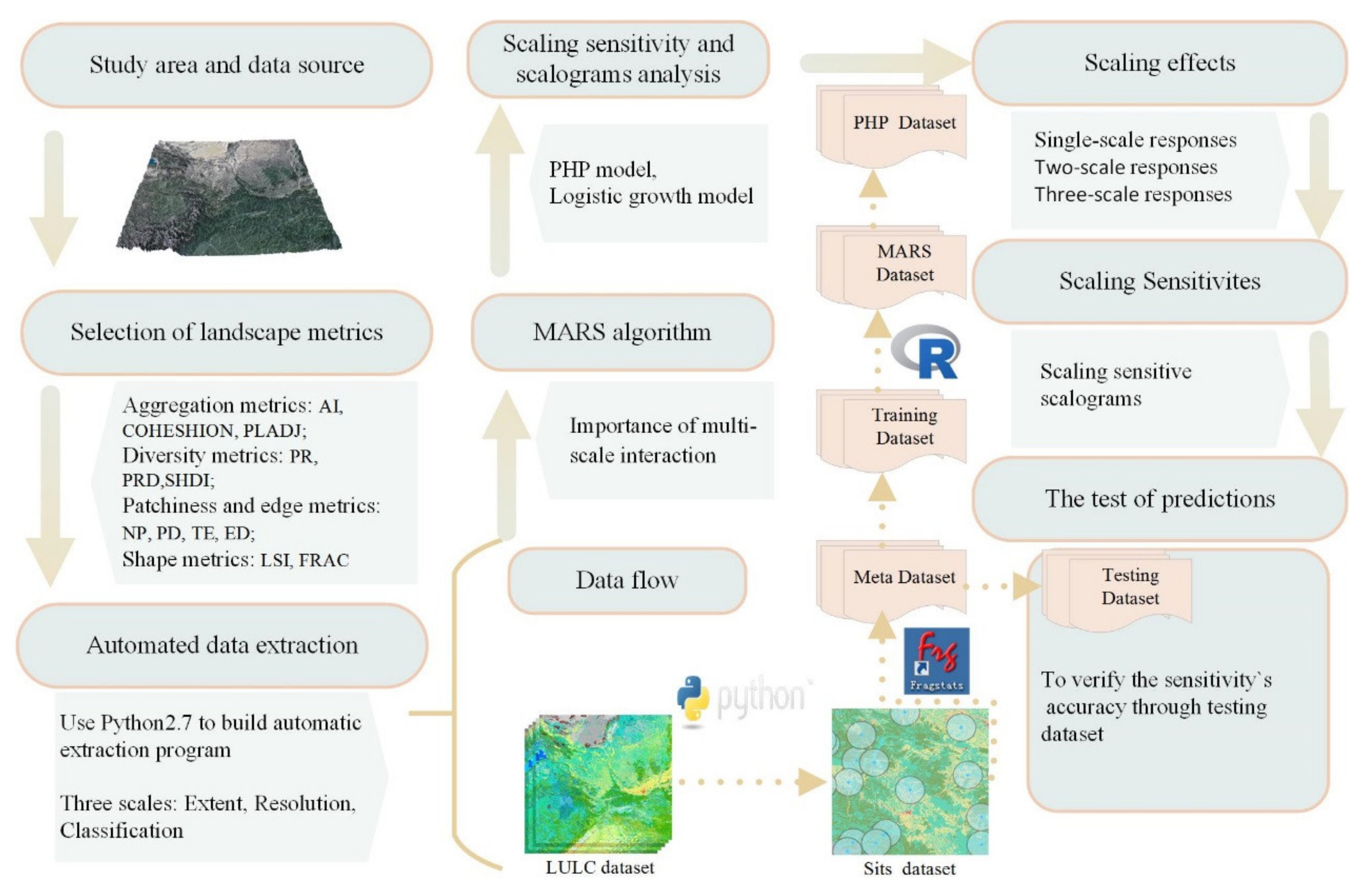
2. Materials and Methods

In this study, the main methodological steps include the data flow, the interpretation of three scale factors, and the analysis of scaling sensitivity (Figure 1). We prepared the LULC data according to this flowchart, wrote automatic sampling procedures, built a large meta dataset, and then studied the scaling response relationships of landscape metrics. The following sub-sections describe each step in detail.

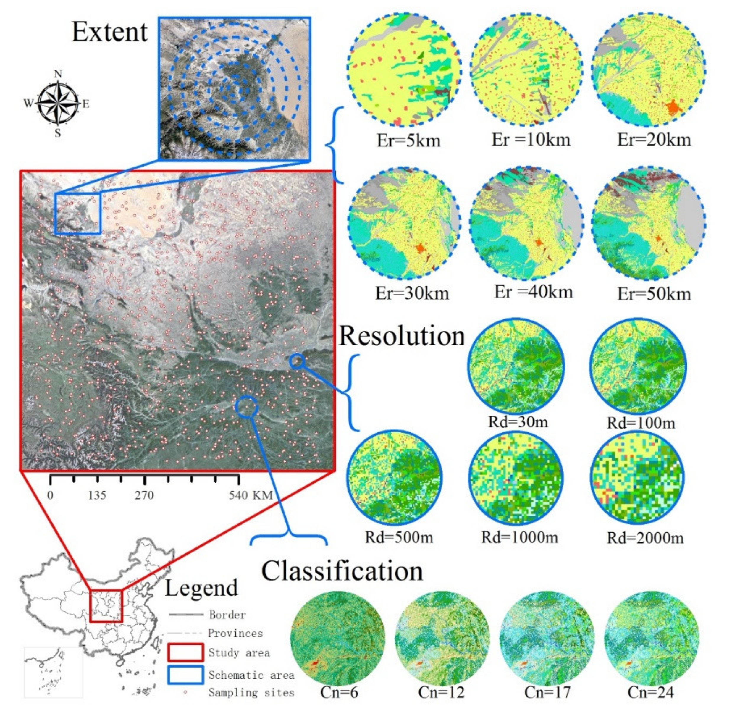
2.1. Study Area and Data Source

The study area was located in the central part of China. This area is one of the richest landscape-diverse regions in the world, including almost all continental landscape categories (e.g., farmland, forest land, desert, glacier, river, and lake). This area contains a part of the Loess Plateau, Tibet Plateau, Sichuan Basin, Tenggeli Desert, Qinling Mountains, and Gaunzhong Plain, covering a geographic area of about 980,000 km², with an elevation range of 50–5600 m. Forest and grass are the main land use classes in this area.

The LULC data (30 m and 1000 m) for this study area were provided by the resource and environmental data cloud platform of the Chinese Academy of Science [30]. The other LULC data were systematically resampled from a resolution of 30 m or 1000 m upwards to 100 m, 500 m, and 2000 m, using the statistical mean aggregation method. The number of landscape classes of those LULC data was then divided into 4 gradients, including 6, 12, 17 and 24 classes, respectively (Figure 2).

2.2. Methods

2.2.1. Selection of Landscape Metrics

A total of 12 landscape-level metrics were selected based on the criteria of commonality and representativeness to quantify the scaling effect and scaling sensitivity on landscape patterns. The landscape metrics could be grouped into 4 categories: aggregation metrics, diversity metrics, patchiness and edge metrics, and shape metrics [31] (

Table 1. The 12 landscape metrics.

Types	Acronym	Name	Units
Aggregation Metrics	AI	Aggregation Index	%
	COHESION	Patch Cohesion Index	Unitless
	PLADJ	Percentage of Like Adjacencies Index	%
Diversity Metrics	PR	Patch Richness Index	Unitless
	PRD	Patch Richness Density Index	/0.01 km2
	SHDI	Shannon’s Diversity Index	Unitless
Patchiness and Edge Metrics	NP	Number of Patches Index	Unitless
	PD	Patch Density Index	/0.01 km2
	TE	Total Edge Index	0.001 km
	ED	Edge Density Index	0.1 km/km2
Shape Metrics	LSI	Landscape Shape Index	Unitless
	FRAC	Mean Fractal Dimension Index	Unitless

). The 12 landscape metrics were batch calculated by the software Fragstats 4.2 using an 8-neighbor rule [32].

2.2.2. Automated Data Extraction

The step of automated data extraction based on Python 2.7 and ArcGIS 10.5 was one of the key steps to implement automatic batch sampling. To accurately study the interactions of multi-scale factors on landscape metrics, we needed big data from sampling sites to accurately capture the fine structural characteristics of complex and heterogeneous landscapes. We set 120 parallel processing programs based on the gradients of three scales (spatial extent, spatial resolution, and classification) and selected 1000 random sampling sites for each processing program (Figure 2). Among them, the spatial extent was clipped to a circular shape centered on random sampling sites with a radius of 5 km, 10 km, 20 km, 30 km, 40 km, and 50 km. Then, we accessed a site’s dataset containing 120,000 sampling maps after the program of automated data extraction was applied to all 120 parallel processing programs with different extent, resolution, and classification gradients in this study. Finally, after the batch calculation, we accessed a big training dataset for multi-scale interaction analysis for 12 landscape pattern metrics on the landscape level.

2.2.3. MARS Algorithm

To determine whether multi-scale interaction effects played an essential role in scaling responses, we used the MARS algorithm to examine the performance of their interactions. MARS adaptively sets a series of ‘basis functions’ to approximate the regression formula through an iterative method [29,33]. The equation of MARS is constructed as a linear combination of the basic functions and their interactions, and the equation can be expressed as:

$$\begin{array}{c}Y=\beta +{\displaystyle \sum }_{k=1}^n{w}_k\times H_k\left(X\right)\end{array}$$

(1)

in which $\mathsf{\beta }$ is constant, $H_k\left(X\right)$ is a basis function, and $w_k$ is the coefficient of the basis function.

We used the earth 5.1.2 packages (http://www.milbo.users.sonic.net/earth/, (accessed on 9 November 2019)) on R 3.5.3 to investigate their interactions for the training dataset, setting the maximum interactions with no separate interaction. Through MARS, we could study the multi-scale dependence issues for each landscape metric and obtain the standard contribution rates of each scale, so that we could perform a more refined quantitative analysis of the multi-scale interaction.

2.2.4. Scaling Sensitivity and Scalograms Analysis

The PHP model can easily extract insights from complex models, exclude some non-target variables’ influences, and reveal the relationship between the outcome and predictors of interest [34]. Therefore, we used the R package of PHP to weaken the interference of the interaction of non-target scales, and then we mainly focused on the response relationship between target scale factors and landscape metrics. Furthermore, we quantitatively analyzed the 3 single-scale effects, 3 pair double-scale effects, and the multi-scale effect of all 3 scale factors. Finally, according to the response relationship between the landscape metrics and these scales, we were able to obtain the response curves and surfaces of landscape metrics to changing scales and interactions.

The scaling sensitivity can be measured by the slope function of the scaling response. Therefore, we used the PHD dataset to fit the smoother single-scale curves, eliminating the interference of other scales, and conducted a quantitative analysis of the sensitivity of landscape metrics. The equation of the 4-parameter logistic growth model is often used for biochemical reactions. In this study, we introduced this model to simulate the smoother single-scale response curves, and the equation can be expressed as:

$$\begin{array}{c}y=\mathrm{d}+\frac{a-d}{1+{(\frac{x}{c})}^b}\end{array}$$

(2)

in which $a$ and $d$ are the theoretical upper and lower limits values of landscape metrics, $c$ is the initial theoretical value, and $b$ is the growth rate.

We derived curves to calculate their slope curves, then used the trigonometric function to get the slope angle curves of absolute slope values. We set the slope angle curves as the quantitative measuring curves for scaling sensitivity. According to the actual applications, we preset the value ranges of extent scale, resolution scale, and classification scale as 1–500 km, 30–10,000 m, and 2–50, respectively. As the value of scale factors increases, the landscape metrics eventually approach the gradual saturation line of its’ growth curve. Thus, according to the value ranges of landscape metrics and those fitting logistic growth curves, we calculated 95% and 99% asymptotic saturation points of the landscape metrics’ value ranges as the critical points [35]. If the scale value was within a 1% threshold of the saturation range (two-sided test), we considered it to be less sensitive to the scale. However, if the scale value exceeded the 5% threshold [11] of the saturation range (two-sided test), we considered it to be significantly sensitive to the scale. Finally, we calculated the sensitive scalograms of landscape metrics and predicted their critical points and thresholds.

To further simulate the scaling sensitivity of multi-scale response relationships, we used the surface slope method to quantitatively analyze the scaling sensitivity of metrics to three scales. After normalizing the PHP dataset of extent scale and resolution scale as 0–1, we used the 3-dimensional surface analysis model on ArcGIS 10.5 to calculate the surface slope angle (using an 8-neighbor rule) of the interaction of extent scale and resolution scale under classification scale, respectively. We could use those simplified fitting response surfaces as the measuring tools for multi-scale sensitivity of landscape metrics.

2.3. Verification of the Scaling Predication

Since the classification scale had the highest consistency and it was difficult to set its gradient, we only tested the other two scales’ scaling sensitivity. In this case, for verification, we set the number of classes to 12, the range of extent radius from 5 km to 100 km, and the range of resolution grain size from 30 m to 3000 m. Then, we extracted 24,000 sampling maps using the automatic sampling process and calculated the 12 landscape metrics in batches. In this case, we obtained a testing dataset of scaling sensitivity, and we could study the changing trends of landscape metrics on the spatial extent scale and resolution scale, respectively. We applied the Leven variance test and the independent Z test to check the differences between the scale gradients. Then, we analyzed the scaling response curves of the testing dataset and verified the scaling sensitivity results.

3. Results

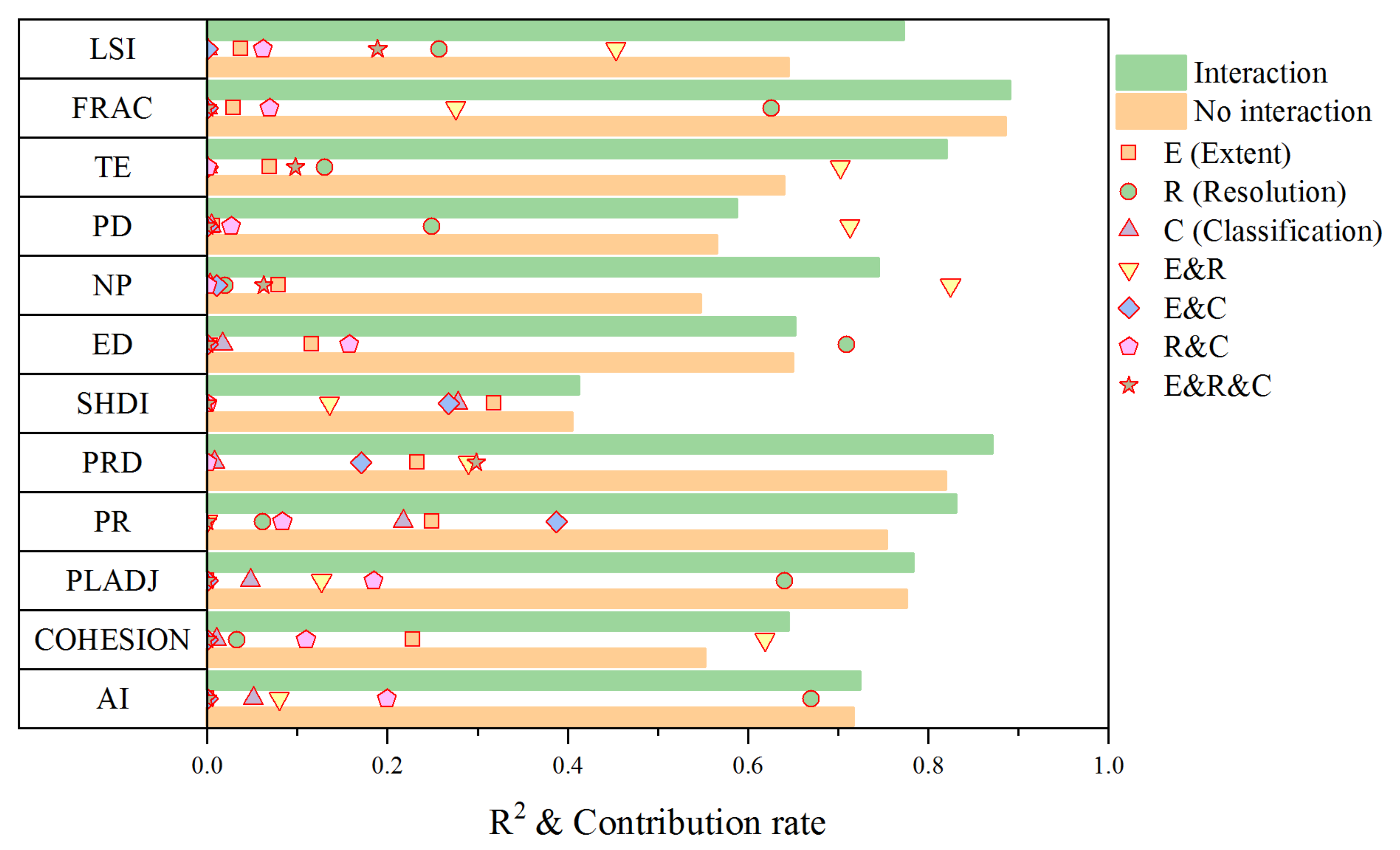
3.1. Importance of Multi-Scale Interaction

Multi-scale interaction widely existed in the scaling effect of landscape metrics, and it strongly affected the interpretation precision of the scaling functions. Comparing the R² of MRAS modes between interaction and no interaction revealed that adopting interactions into scaling functions could improve their goodness-of-fit (R²) for 12 landscape metrics, especially NP, LSI, TE, and COHESION (Figure 3). The contribution rate of interactions was mainly between 0.2 and 0.9. Among them, the average contribution rate of 12 metrics’ multi-scale interaction was 0.55, which showed that the multi-scale interactions’ contribution was greater than the contribution of scales in isolation (Figure 3). The three single-scale factors and their interactions together determined the scaling responses of landscape metrics. There are three two-scale interactions and one three-scale interaction in this study. Among them, the interaction between extent and resolution was often the primary contributing factor in multi-scale interaction, especially for five metrics such as ED, NP, PD, COHESION, and LSI. The resolution scale was also the most significant single-scale contributing factor for most landscape metrics (e.g., TE, FRAC, AI, and PLADJ), while the classification scale often had a weak impact on most landscape metrics.

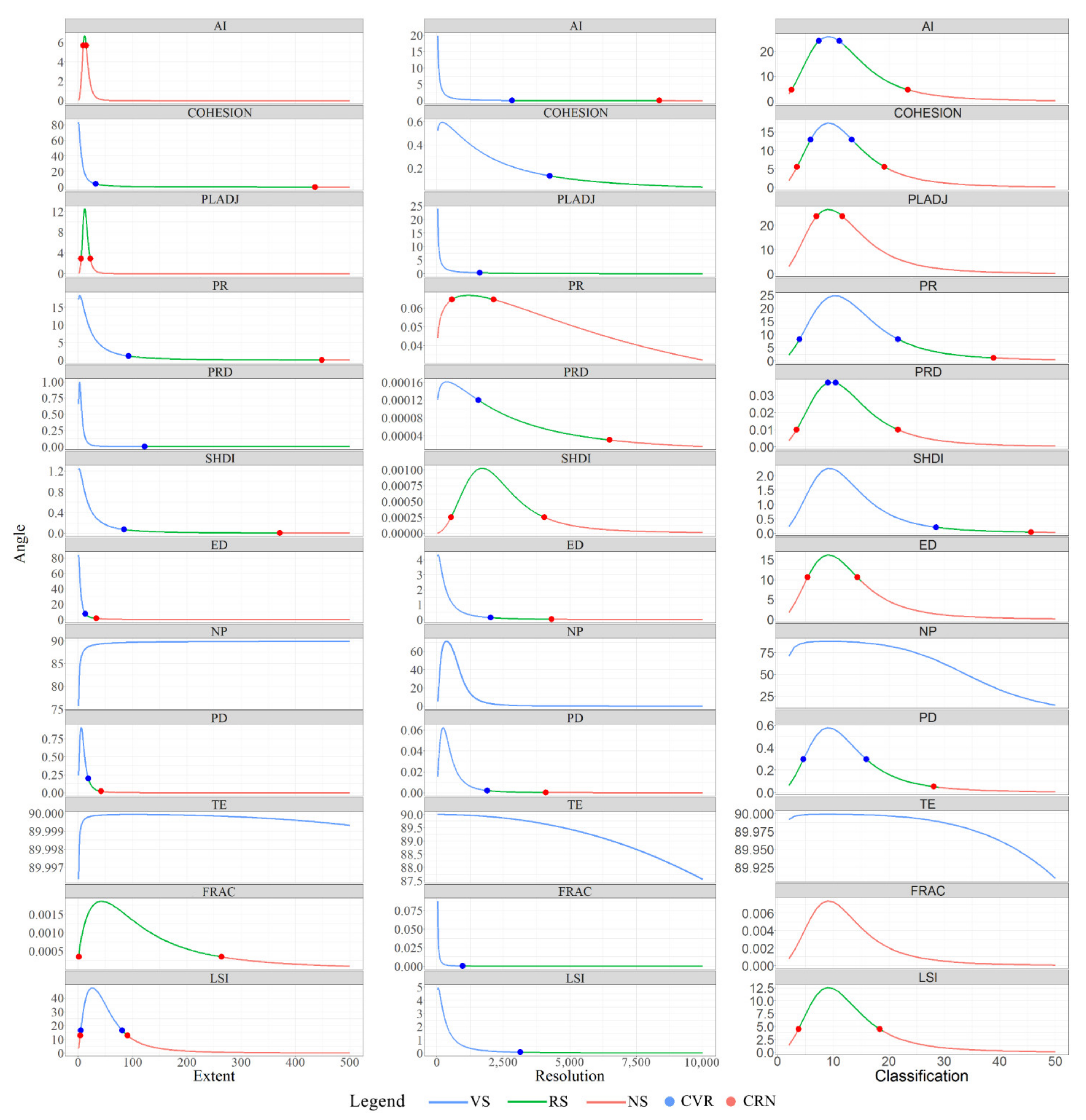
3.2. Scaling Effects

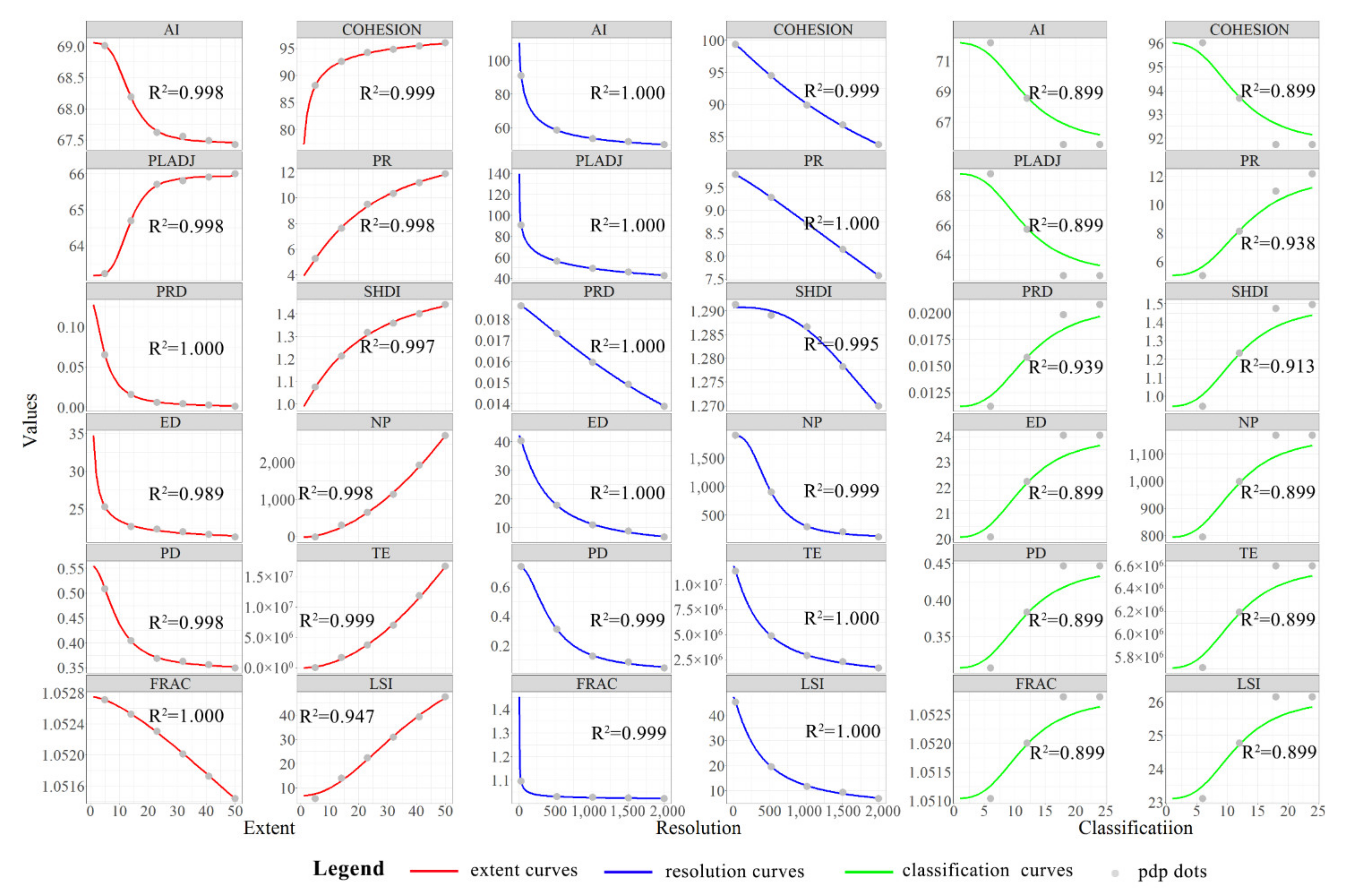
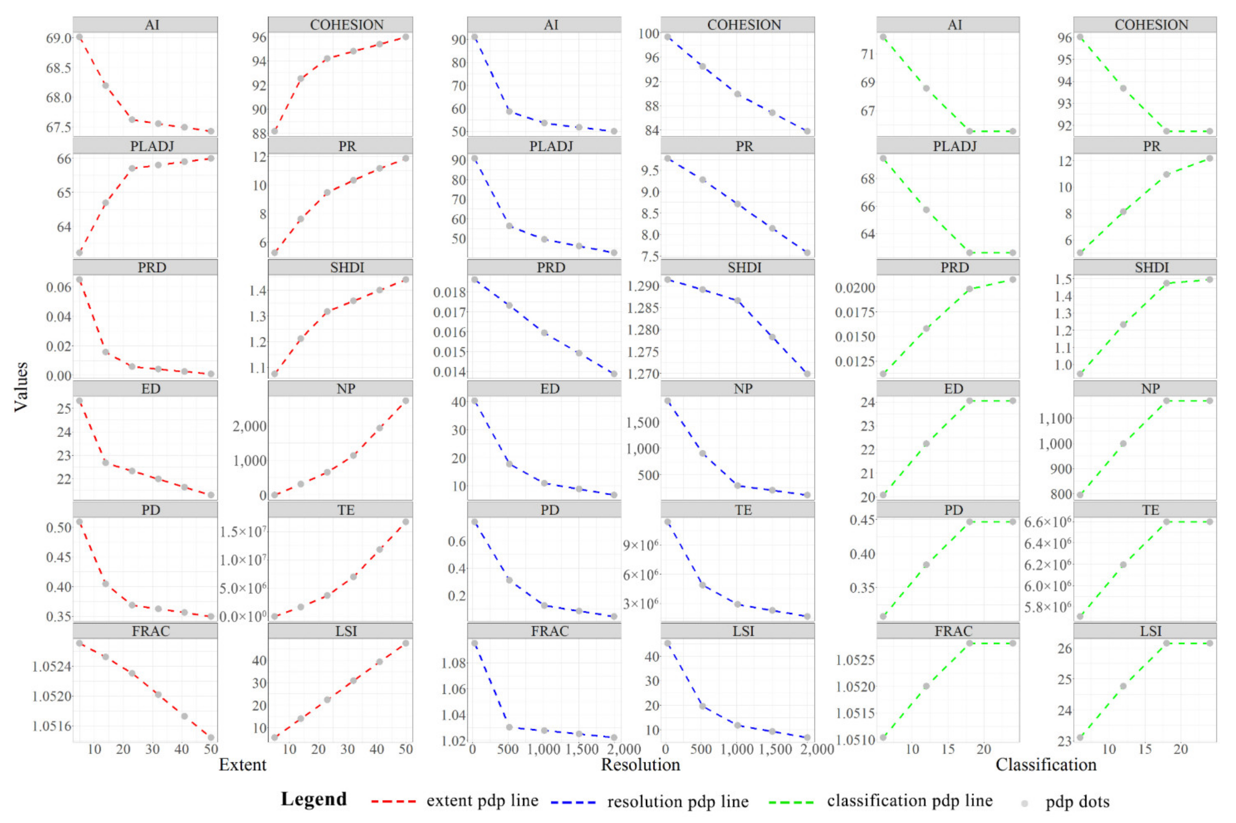
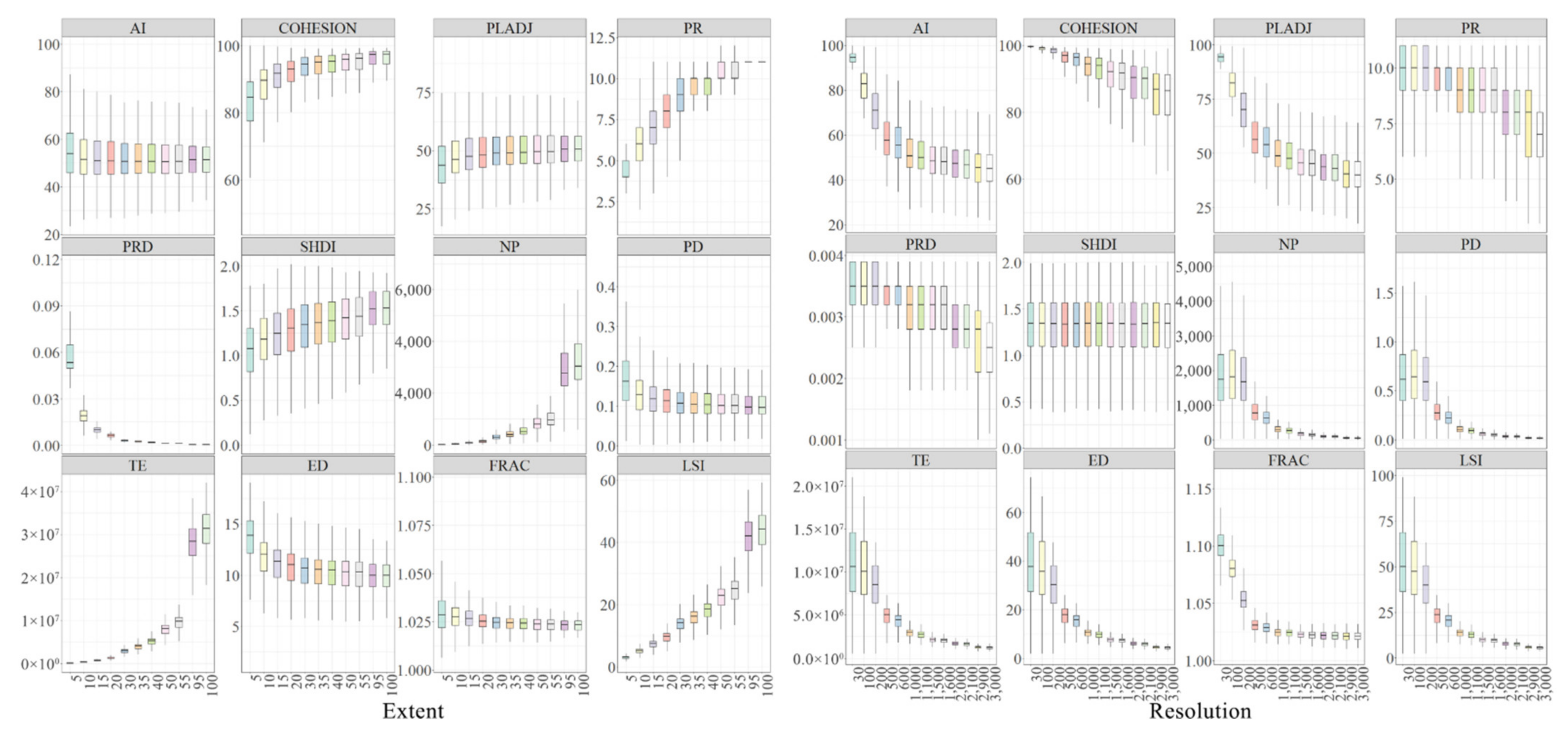
3.2.1. Scaling Responses of Three Scales

The single-scale response lines, which excluded the interference of other scale factors using MARS and PHP models, more accurately displayed the single-scale response relationships in an actual scene (Figure 4). As the values of extent, resolution, and classification increased, the landscape metrics changed differently. Among them, the scaling response lines of extent scale to landscape metrics were most inconsistent on direction, but the shapes of classification response lines of scale had the highest consistency, whose inflection points appeared at 17. The resolution scale was negatively correlated with all landscape metrics, that is, as the grain size of resolution became coarser, the values of the above 12 landscape metrics all became smaller.

The scaling responses of 12 landscape metrics to three scales also varied considerably. First, the influence degree and value range of three single-scale factors to the same landscape metric had distinct differences. We take AI as an example to show three scales’ scaling effects, the resolution scale had the greatest impact on AI, whose value range was from 50 to 90. However, the value range of AI on extent scale was only from 67.5 to 69. It showed that the scaling effect of extent was smaller than the resolution’s effect for the metric of AI. Second, those response directions of scaling effects were discrepancies to some degree. The scale factors of extent and classification had different response directions to 12 landscape metrics, such as the extent scale being a positive increase for PLADJ, while it was a negative decrease for FRAC. Third, the effective ranges of scaling effects were also inconsistent. Taking PLADJ as an example, the effective range of the extent scale radius was mainly within 30 km; if it exceeded 30 km, the scaling effect of resolution decreased to become weaker and weaker. Based on the single-scale response lines of 12 metrics, we found that the scaling effects of three single-scale factors usually differed in intensity and direction, even to the same landscape metrics.

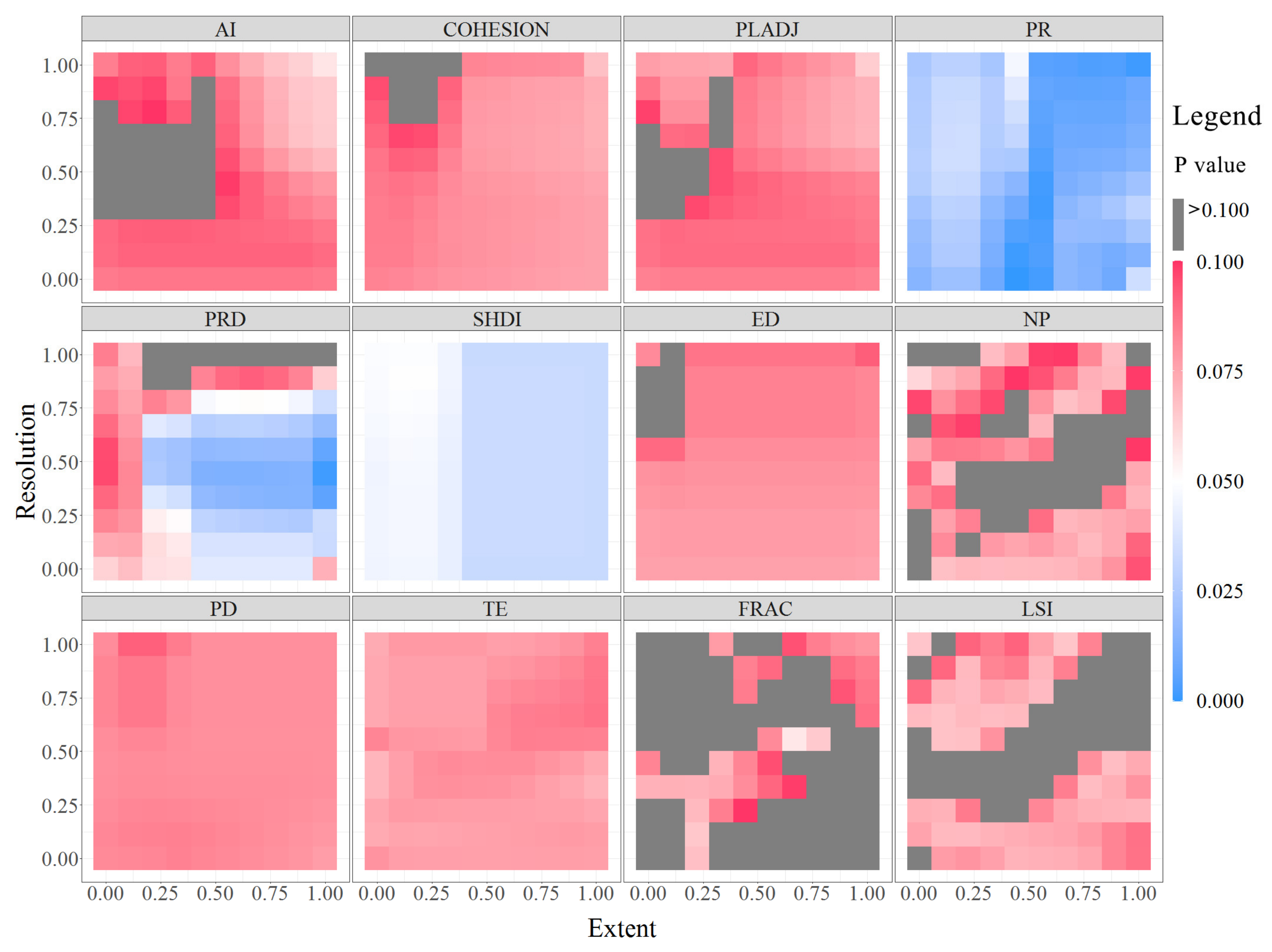
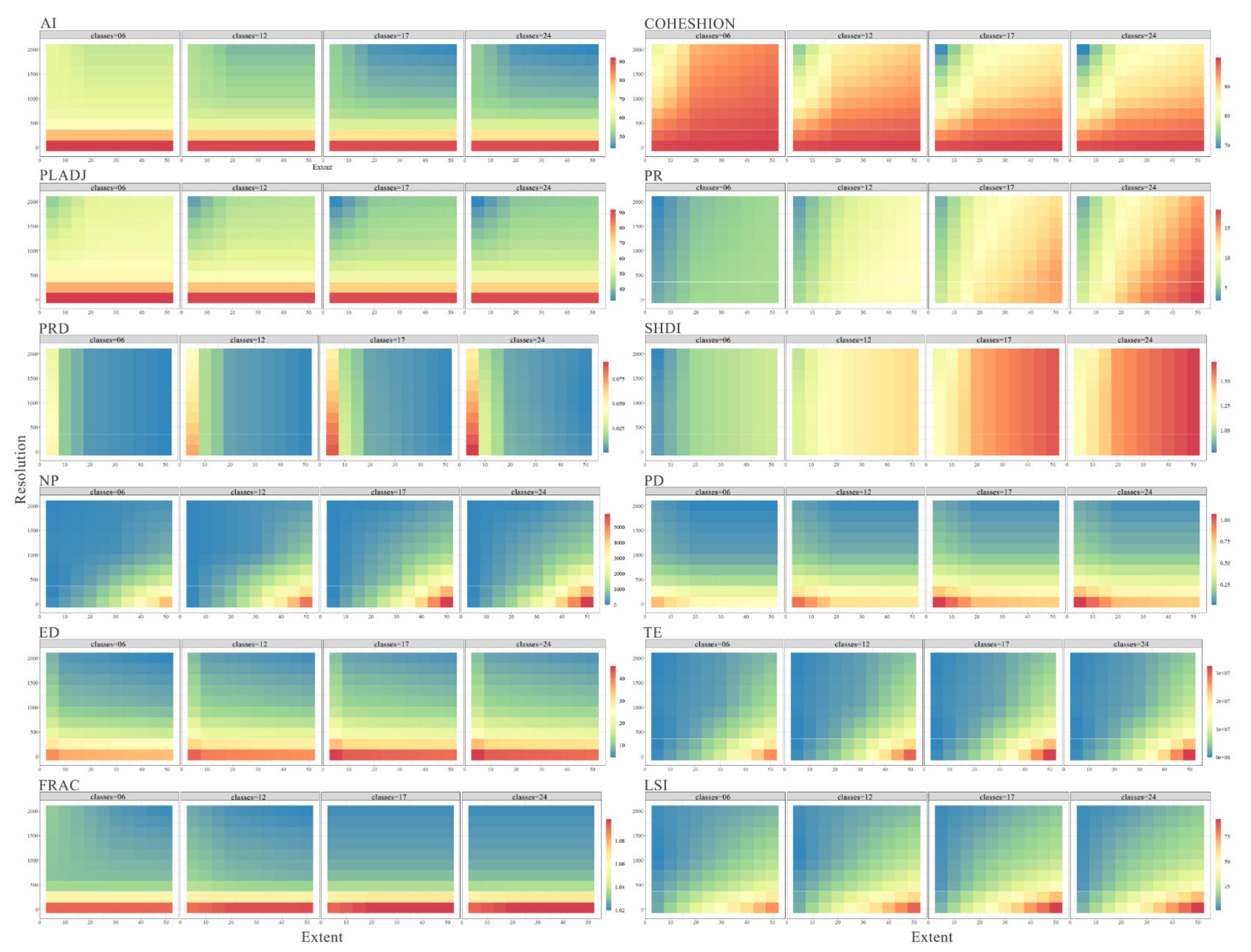
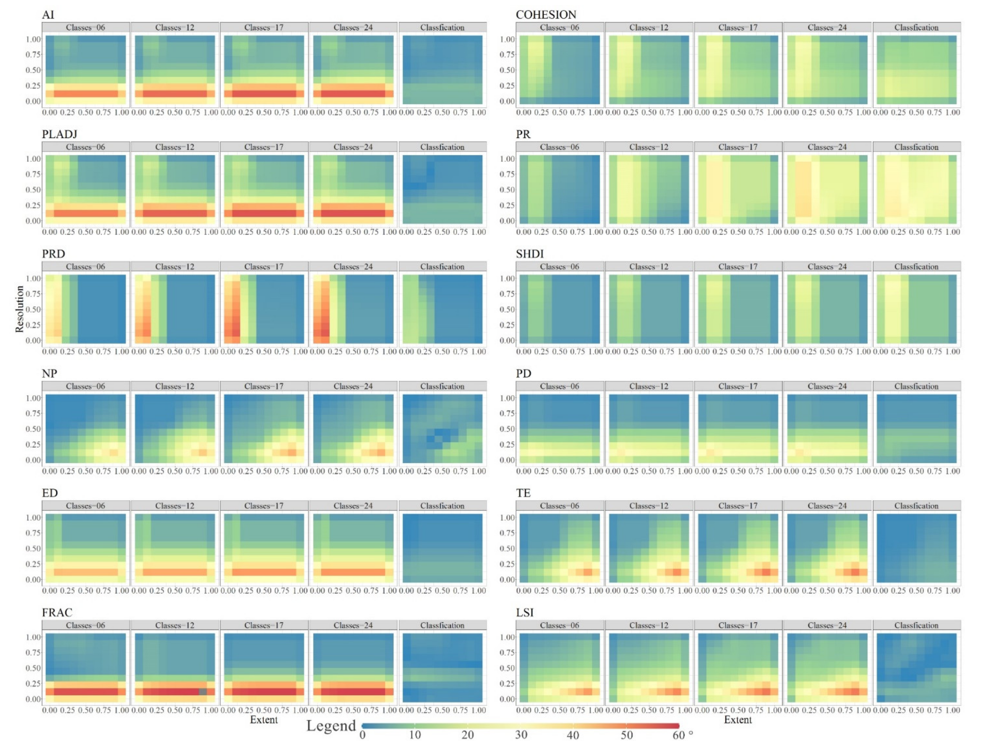
3.2.2. Performance of the Two-Scale Interaction

The two-scale interaction was the principal manifestation in multi-scale interactions; the interaction between resolution scale and extent scale especially had the strongest scaling response relationship in most metrics. According to the response performance of the two-scale interactions in Figure 5, we mainly divided them into three effect types: synergistic effect, antagonistic effect, and single-scale dominance effect. Among them, the synergistic effect referred to the cooperative response of two scale factors to corresponding landscape metrics, such as the values of PR increasing with the radius of extent scale and the number of classes in the classification scale, and their scaling effects were cumulative for PR. The antagonistic effect was described as “push–pull”, that is, these two scales had an opposite response to landscape metrics. The single-scale dominance effect meant no remarkable two-scale interaction or that one of two scales was too feeble to affect landscape metrics, such as the two-scale interaction between resolution and classification in SHDI, FRAC, and LSI.

The scaling responses of two-scale interactions showed that most landscape metrics were simultaneously affected by multiple scales, and the responses of different metrics to changing scales were also quite different. The results also showed that the primary two-scale interaction had an antagonistic effect, especially as the spatial resolution usually had an inhibitory influence on other scales. We took COHESION as an example: its’ two-scale interaction between the scales of extent and resolution was an antagonistic effect, whose values were positively correlated with the extent but negatively correlated with the resolution. The COHESION scaling curves of extent were extremely different at different degrees of resolution, such as when the grain size was 30 m, the scaling curve of extent was almost a horizontal line, and when the grain size was 2000 m, the scaling curve of extent was similar to a parabola (Figure 5). The results showed that most individual scaling effects were affected by other scale factors; thus, most scaling responses of landscape metrics were inconsistent across the whole spectrum of scale, except for the resolution scale of SHDI.

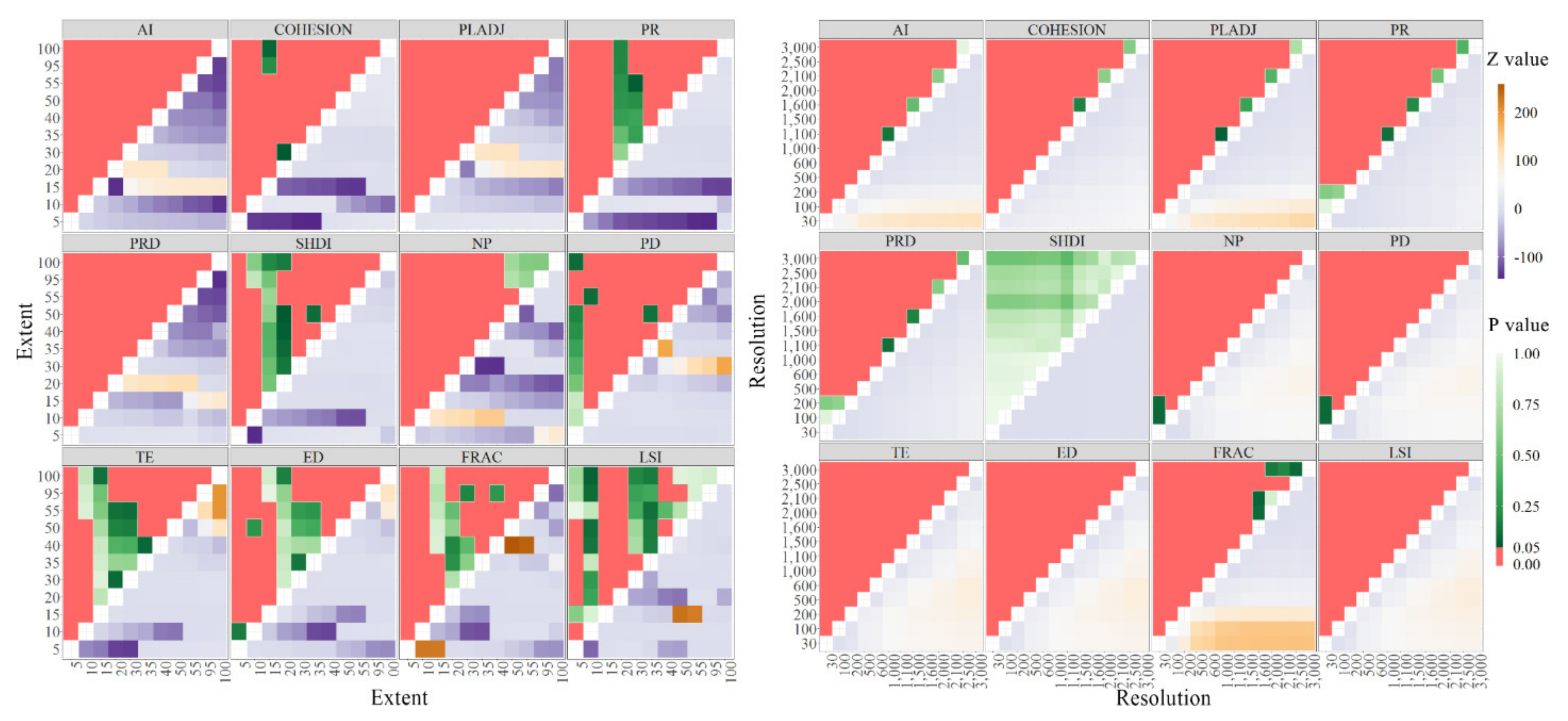
3.2.3. Comprehensive Analysis of Three-Scale Interaction

Compared to the two-scale interaction, the interaction between three scales had more complicated scaling response relationships, presenting intricate and complex multi-dimensional graphical distribution characteristics in Figure 6. Based on those graphic characteristics, we grouped them into four types: (1) vertical changing trends were mainly affected by the extent’s scaling effect (e.g., SHDI); (2) horizontal changing trends varied substantially along the resolution scale (e.g., ED, and FRAC); (3) diagonal changing trends had a significant two-scale interaction between extent and resolution (e.g., NP, TE, PD, and LSI); and (4) compound changing trends, such as AI, PLADJ, and PR, mixed with several changing characteristics along the classification scale. Taking PR as an example, it presented a vertical changing trend when the class number was less than 12, but a diagonal changing trend when it was beyond the critical range. According to the changing gradient of classes, the results showed that nearly half of the metrics were insensitive to the classification scale, and most metrics were mainly affected by the scaling effect of two-scale interaction (Figure 6). However, the others, especially COHESION, PLADJ, and PR, had an obvious combined response of three-scale interaction. In short, the results indicated that the scaling responses of landscape metrics usually received a comprehensive effect of multi-scale interaction in the actual scenario.

3.3. Scaling Sensitivities

3.3.1. Scaling-Sensitive Scalograms of Three Scales

Based on the single-scale logistic growth curves (Figure A1) and their slope curves (Figure A2), we were able to quantitatively simulate the scaling sensitivity scalograms and forecast the scaling sensitivity of landscape metrics to three scales. The results showed that only a few metrics (e.g., NP and TE) remained highly sensitive to the three scales throughout the whole spectrum of scale, while others were only sensitive in a certain range of scale (Figure 7). Among them, AI, PLADJ, and FRAC were insensitive to the extent scale, PR and SHDI were insensitive to the resolution scale, and PLADJ, ED, FRAC, and LSI were also insensitive to the classification scale. We found that the scaling-sensitive curves of three scales were almost different from each other. Among them, the scaling-sensitive scalograms of the resolution were extremely heterogeneous to different metrics. Although the sensitivity of most metrics decreased with the coarser grain size, their sensitivity thresholds and curve shapes differed significantly. However, the sensitive scalograms of classification had the highest consistency, most of which were inverted U-shaped curves, and their scaling sensitivity reached the highest when the class number of classification was about 10. The difference of extent was between the other two scales, and their optimal sensitive segments almost ranged from 10 km to 40 km.

We found that the scaling-sensitive characteristics of metrics were almost specific, and even similar or the same type of metrics were also significantly different. The results showed that most landscape metrics had an optimal range or sensitive threshold for corresponding scales (Figure 7). When the value of scales exceeded the threshold, their scaling sensitivity would tend to stabilize; especially in addition to NP and TE, the scaling sensitivity value of most other metrics would approach 0°. It implied that the scaling effects had an optimal and best value range of three scales, and beyond the threshold (e.g., critical points) the scaling sensitivity would become lower and lower; at this time, some landscape metrics would become blurred by losing their fine spatial information regarding landscape heterogeneity. The scaling-sensitive scalograms quantitatively explained the response relationships of scaling sensitivity, and they predicted the optimal sensitivity range of metrics to three scales. Therefore, the results also offered a guideline for the selection of suitable landscape metrics and an optimal scale range. We suggested that the blue line segments corresponding to the optimal range of three scales in Figure 7 should be preferred to enhance the metrics’ scaling sensitivity. Though, the insensitive ranges of scales should be avoided as much as possible in the application of landscape metrics.

3.3.2. Scaling Sensitivity Based on Three-Scale Interaction

To further explore the scaling sensitivity of metrics, we simulated their comprehensive scaling-sensitive maps based on the three-scale interactions and surface analysis model. As the degree of interaction increased, the scaling response relationship became more complicated. Figure 8 more intuitively shows the scaling sensitivity of metrics to three-scale interaction, and it presents the red area as the best range with the highest scaling sensitivity. The linear changing trend statistical significance of extent and resolution scaling sensitivity along the classification (Figure A3) showed that most landscape metrics had low sensitivity to classification, except for SHDI, PR, and PRD. The results further indicated that the scaling effects generally had a threshold interval of sensitivity or insensitivity, and the scaling sensitivity was often dominated by the multi-scale interaction.

3.4. The Test of Predictions

By comparing the predictions of scaling sensitivity (Figure 7) and the test dataset (Figure 9), we verified the accuracy of scaling sensitivity for the extent scale and the resolution scale. The results showed that the statistical distribution of most landscape metrics conformed to our expectations, and it indicated that the scaling-sensitive scalograms could be used as a guideline in the study of landscape ecology. We took SHDI as an example; it had the smallest difference on the resolution scale, and the Z test in Figure A4 also verifies that their differences between groups on grain size were not significant (p < 0.05). The results showed that the scaling prediction of SHDI, shown in Figure 7, was accurate. Meanwhile, we found that the maximum Z value of LSI on the adjacent extent scale gradient was from 30 km to 35 km, which was also in line with the scaling prediction. Although some Z test results did not meet the scaling predictions, such as PRD and TE, most landscape metrics, shown in Figure 9, were still consistent with Figure 7. For most landscape metrics, the predictions of scaling sensitivity in highly sensitive segments and insensitive segments, shown in Figure 7, were reliable, but there were some deviations on sensitive transition segments, whose magnitude might relate to multi-scale interaction.

4. Discussions

4.1. Multi-Scale Interaction

Natural processes always operate across various spatiotemporal scales, and thus, multi-scale codependence relationships are the cornerstone of understanding ecological processes [36,37]. Although many models have been used to investigate response relationships of multiple scales since the 1980s [6,20], the most widely used methods (e.g., variance analysis) are still insufficient to clearly reveal the interactions between scales [25,28]. In this study, we found that using the MARS and PHP models for multi-scale interaction can effectively improve the ability to quantify the scaling effects of metrics. Moreover, the 12 landscape metrics were seriously affected by multi-scale interaction, which indicated that the responses of metrics to changing scales were highly dependent on the scales and the interactions between scales. Therefore, the scaling issues not only need to comprehensively consider the scaling responses of corresponding scales but also need to consider the interactions between these scales. However, most landscape metrics scaling effect studies, based only on scales themselves without considering their multi-scale interaction, might have caused a serious misunderstanding of landscape patterns.

Investigating the scaling effect of a single scale in isolation would be disturbed by other scale factors. Although the multi-scale interaction of landscape metrics had been focused on by some researchers [11,28], many traditional methods used in scaling issues assumed the independence of the observations in advance [25]. In particular, some researchers implied there to be no complex interaction for landscape metrics’ scaling responses, and the main effects were always in one direction [28]. However, this study testified that the interactions between scales were widespread in all landscape metrics containing complex scaling responses. Furthermore, the results also showed that the average contribution of multi-scale interaction was bigger than the contribution of three single scales on scaling responses. In summary, ignoring multi-scale interaction will lose some vital information regarding landscape patterns; therefore, we emphasize that multi-scale interaction plays an important role in landscape metrics.

4.2. Scaling Responses of Metrics to Resolution, Extent, and Classification

The response relationships of landscape metrics to scales are mainly affected by spatial extent, spatial resolution, and classification system [14]. However, most previous studies about multi-scale analysis mainly focused on the extent and the resolution [38], and only a few of them were concerned with classification. Although these first two scales and their interactions are the main contributors to the scaling responses for most landscape metrics, the interactions between the classification scale and others are also crucial for SHDI, PR, LSI, etc. Guiding the translation or extrapolation of spatial information from one scale to another, especially across multi-scale interaction, is a challenge. Previous scaling functions presented a set of complicated nonlinear response relationships among metrics, resolution, extent, and even classification [23]. Although these scaling functions adopted multi-scale analysis methods, most of them did not take into account their interactions. This study showed that the scaling responses of metrics to three scales are often not isolated but rather mainly depend on multi-scale interaction. Therefore, the lack of multi-scale interaction may lead to an unclear conclusion of scaling responses. For example, some studies suggested that metrics changed considerably with increasing grain size and exhibited consistent patterns over a wide range of spatial resolution [25]. This was not consistent with our study, and we found that most landscape metrics’ scaling effects had effect boundaries, and when the grain size exceeded the critical point, the corresponding metric was nearly unchanged. Some studies believed that the coarser grain size could be used to a larger spatial extent, but we found this phenomenon mainly depended on whether grain size was the largest driving force of the scaling effects, such as PR and SHDI not being sensitive to resolution.

In the past, the selection of scale ranges mainly focused on the resolution, while often ignoring extent and classification. In particular, most studies ignored the effect boundary of spatial extent. We found that most landscape metrics were not suitable for application at a large spatial extent. For example, when the radius of extent exceeded 100 km, half of the 12 landscape metrics were shown to lose sensitivity (Figure 7 and Figure 9). Meanwhile, the class number of classification was not the more the better. Generally, the optimal range of classification was from 5 to 30. In this study, we divided 12 metrics into four types based on the scaling responses of multi-scale interaction (Figure 6) and the kind of compound changing trends that had the most complex scaling performance. Therefore, we can say that the complex metrics (e.g., COHESION and PLADJ) often involve more complicated interactions than other metrics. In contrast, some concise metrics (e.g., NP and TE) are easier to measure their scaling responses [39]. It is for this reason that some researchers have always believed complex metrics to be unpredictable or limited. Some studies showed that the scaling response of the landscape metric to the extent scale was more challenging to predict than the resolution scale [40]. However, we found that these responses to both scales could be better predicted by multi-scale interaction analysis.

4.3. Multiplicity of Scaling Functions

Until now, most researchers have not formed a unified understanding of the scaling function to certain responses, with some of their findings being contradictory [41]. According to the R² of scaling functions to the whole spectrum or a limited range of scales, Wu [16] and Xu et al. [23] grouped them into three types: predictable across the whole spectrum, predictable in a limited range, and unpredictable. Additionally, they used a series of functions to fit the scaling responses between metrics and changing scale one by one. Compared with other simple functions, the logistic growth function has a risk of overfitting. However, we achieved good results with a logistic growth function for all metrics on the whole spectrum of three scales. For example, Pablo Arganaraz and Entraigas [42] used four functions (e.g., liner, power, logarithmic, and exponential) to conduct groundbreaking research on the scaling response for many landscape metrics, but we show these four function curves that can be regarded as a segment of logistic growth curves in Figure A1. We believe that there are three aspects that can be responsible for this contradiction: (1) the multi-scale interaction is not considered, even if the multi-scale analysis method is adopted [42], (2) the scale range is too small to cover the real scaling response curve, so that the fitting functions obtained in different intervals of scale value are inconsistent, and (3) the landscape heterogeneity is too high, or the amount of sampling sites is too small, which will cause severe deviations between the sampling data and the actual scene.

The fitting data (PHP dataset), which has reduced the interferences of multi-scale interaction on the non-target scale, is better than the original dataset in terms of revealing the scaling responses of landscape patterns. A unified scaling function may also make it easier to explain the internal mechanism than a series of different functions. In this paper, Figure A1 reveals that as the value of three scales increases, most landscape metrics will tend towards a stable state. Because landscape metrics represent the spatial heterogeneity information of landscape patterns [3], this means that the reduction in spatial heterogeneity will lead to the loss of fine spatial information with the increase in scale. Compared with other functions, the logistic growth function may be the closest to the nature of landscape patterns, that is, the scaling response of metrics is essentially caused by spatial heterogeneity. With the increase in scale, spatial heterogeneity information will be aggregated into homogenized noise. Therefore, although the scaling response performances of metrics are different, each of them is a projection of spatial heterogeneity information on a certain dimension.

4.4. Robustness of Scaling-Sensitive Scalograms

Although some previous studies have recognized the significance of interactions, they have failed to use effective methods to conduct a detailed investigation of scaling sensitivity. Landscape ecologists agree that a clearer response relationship of metrics to changing scales can help researchers to obtain the optimal range of scale [43]. This study clearly explained multi-scale interaction relationships and extracted single-scale responses from compound multi-scale interaction to quantitatively measure landscape metrics scaling sensitivity. We concisely improved the understanding of scaling sensitivity and offered some quantitative scalograms for landscape metrics (Figure 8). However, the interference of multi-scale interaction was not eliminated; thus, there are still some biases in the prediction results of scaling sensitivity. The robustness of scaling sensitivity can be rectified by adjusting their critical points [24]. In turn, the thresholds (i.e., 1% and 5%), which are regarded as the judgment of the degree of sensitivity, can also be optimized according to the robustness. Most previous studies used a small number of samples to study the scaling responses of landscape metrics [24,26]. However, the high spatial heterogeneity of landscape patterns may cause the excessive dispersion of sampling data, leading to statistical deviations in some areas. Therefore, large amounts of training data containing 120,000 samples were used to increase the size of the traditional sampling data by several orders of magnitude in this study. We believe that big data analysis can enhance the robustness of scaling sensitivity, thereby avoiding the statistical bias of investigative data.

Some studies have hoped to construct the proper scaling response functions of landscape metrics’ values. However, Frazier [11] stated that the predicted deviation of landscape metrics’ values obtained by scaling functions is too large to predict the exact value of metrics. Our findings support the idea that it is difficult to adequately transfer landscape metrics’ values from one scale to another due to the complexity of multi-scale interaction and the highly heterogeneous landscape. Although it is impossible to predict the right value of metrics, we can more accurately predict their trends of scaling sensitivity by scaling functions.

4.5. Limitations and Future Perspectives

The selection of landscape indicators may affect the conclusion of this study. Although we selected 12 commonly used landscape indicators in four types for research, there are many various landscape indicators in landscape ecology. The 12 landscape metrics in this study cannot cover the scaling sensitivity characteristics of all landscape indicators. Therefore, the results of this study mainly reflect the scaling sensitivity characteristics of these 12 landscape indicators. In addition, although we used a new method to measure the multi-scale interaction relationship, the PHP model tries to weaken the interference of non-target scales rather than fully eliminate the interference of non-target factors. Therefore, the landscape metrics’ scaling-sensitive scalograms (Figure 7) are still affected by interactions to some extent. Finally, the spatial heterogeneity between different ecosystems may limit the application of this research. This study area includes various landscape classes, such as forest, grassland, desert, farmland, etc. Furthermore, it should be warned that the scaling-sensitive scalograms and other scaling findings in this study may be specific to general landscape regions. For example, the coastal wetland ecosystem has its unique landscape pattern characteristics, and this study’s general conclusions may not be directly used.

Although the multi-scale interaction method mainly focused on the scale sensitivity of 12 metrics in this study area, this method is generic and applicable to the broader fields of land science and landscape ecology. In particular, it can be further applied to other landscape metrics and unique ecosystems. Therefore, it is necessary to construct corresponding scaling-sensitive scalograms according to different ecological regions, such as mountain forest ecosystems. We also hope to further study the multi-scale interaction of landscape indicators at national and global scales. In general, we still recommend that it is feasible to use the scaling-sensitive scalograms as an application guideline on how to select an appropriate landscape metric or an optimal range of scales.

5. Conclusions

Multi-scale analysis can reveal the scaling response between landscape metrics and scales. However, most researchers investigate the scaling response of landscape metrics to changing scales in isolation, ignoring their multi-scale interaction. The lack of multi-scale interaction analysis seriously loses some spatial heterogeneity information between multiple scales, leading to some systematic biases. This study systematically investigates whether multi-scale interaction is important for scaling effect and scaling sensitivity. Fully considering the impact of multi-scale interaction could significantly reduce some contradictions and uncertainties of landscape metrics. The results show that the multi-scale interaction’s average contribution rate of 12 metrics was 55%. Therefore, the multi-scale interaction analysis was important for the scaling response, which should not be ignored. We found the scaling effects of the three scales were significantly different. In general, the resolution was the primary driving scale, such as TE, FRAC, AI, and PLADJ, being mainly affected by changing grain size. Meanwhile, the classification had the highest consistency to 12 metrics, and the scaling sensitivity was highest when the class number was around 10. As the dimensions of scales increased, the scaling responses of multi-scale interactions became more complicated, and their scaling effects were often in a different direction, such as the antagonistic effect being the primary type of two-scale interaction. This study contributed to enhancing our understanding of the scaling effects and sensitivity affected by multi-scale interaction, and the results also demonstrated the need for the interactions between multiple scales to be emphasized in the studies of landscape patterns.

The spatial heterogeneity of landscape patterns might cause a certain degree of statistical bias in sampling analysis. We constructed large amounts of training data through an automated data extraction program. This study showed that the big data analysis method could improve the robustness of the results. Therefore, we suggested that big data statistics and analysis methods should be emphasized in landscape pattern research.

Meanwhile, we believed that some fine spatial information of landscape heterogeneity had been lost in the process of scaling transfer, and thus it was impossible to obtain the right values of landscape metrics through scaling functions. However, we studied the scaling effects based on the multi-scale interaction analysis and constructed the scaling sensitivity scalograms according to the scaling curves. The scaling-sensitive scalograms could provide sufficient predictive information on the scaling response relationships of landscape metrics to multiple scales. These scalograms can be used as a general guideline for selecting appropriate landscape metrics and screening the optimal scale ranges. Especially in landscape planning and land management, this predictive information can help researchers and decision-makers to reduce some systematic biases and improve the accuracy of landscape metrics’ application.

References

1. Liu, Y.; Wei, X.; Li, P.; Li, Q. Sensitivity of correlation structure of class- and landscape-level metrics in three diverse regions. Ecol. Indic. 2016, 64, 9–19. [Google Scholar] [CrossRef]
2. Almenar, J.B.; Bolowich, A.; Elliot, T.; Geneletti, D.; Sonnemann, G.; Rugani, B. Assessing habitat loss, fragmentation and ecological connectivity in Luxembourg to support spatial planning. Landsc. Urban Plan. 2019, 189, 335–351. [Google Scholar] [CrossRef]
3. McGarigal, K. Landscape pattern metrics. In Encyclopedia of Environmetrics; John Wiley and Sons: Hoboken, NJ, USA, 2013. [Google Scholar] [CrossRef]
4. Medeiros, A.; Fernandes, C.; Goncalves, J.F.; Farinha-Marques, P. Research trends on integrative landscape assessment using indicators—A systematic review. Ecol. Indic. 2021, 129, 107815. [Google Scholar] [CrossRef]
5. Mairota, P.; Cafarelli, B.; Boccaccio, L.; Leronni, V.; Labadessa, R.; Kosmidou, V.; Nagendra, H. Using landscape structure to develop quantitative baselines for protected area monitoring. Ecol. Indic. 2013, 33, 82–95. [Google Scholar] [CrossRef]
6. Hainesyoung, R.; Chopping, M. Quantifying landscape structure: A review of landscape indices and their application to forested landscapes. Prog. Phys. Geog. 1996, 20, 418–445. [Google Scholar] [CrossRef]
7. Hesselbarth, M.H.K.; Sciaini, M.; With, K.A.; Wiegand, K.; Nowosad, J. Landscapemetrics: An open-source R tool to calculate landscape metrics. Ecography 2019, 42, 1648–1657. [Google Scholar] [CrossRef] [Green Version]
8. Wu, J. Key concepts and research topics in landscape ecology revisited: 30 years after the Allerton Park workshop. Landsc. Ecol. 2013, 28, 1–11. [Google Scholar] [CrossRef]
9. Huais, P.Y. Multifit: An R function for multi-scale analysis in landscape ecology. Landsc. Ecol. 2018, 33, 1023–1028. [Google Scholar] [CrossRef]
10. Yang, M.; Gao, X.; Zhao, X.; Wu, P. Scale effect and spatially explicit drivers of interactions between ecosystem services—A case study from the Loess Plateau. Sci. Total Environ. 2021, 785, 147389. [Google Scholar] [CrossRef]
11. Frazier, A.E. A new data aggregation technique to improve landscape metric downscaling. Landsc. Ecol. 2014, 29, 1261–1276. [Google Scholar] [CrossRef]
12. Baldwin, D.J.B.; Weaver, K.; Schnekenburger, F.; Perera, A.H. Sensitivity of landscape pattern indices to input data characteristics on real landscapes: Implications for their use in natural disturbance emulation. Landsc. Ecol. 2004, 19, 255–271. [Google Scholar] [CrossRef]
13. Kopp, D.; Allen, D. Scaling spatial pattern in river networks: The effects of spatial extent, grain size and thematic resolution. Landsc. Ecol. 2021, 36, 2781. [Google Scholar] [CrossRef]
14. Simova, P.; Gdulova, K. Landscape indices behavior: A review of scale effects. Appl. Geogr. 2012, 34, 385–394. [Google Scholar] [CrossRef]
15. Buyantuyev, A.; Wu, J. Effects of thematic resolution on landscape pattern analysis. Landsc. Ecol. 2007, 22, 7–13. [Google Scholar] [CrossRef]
16. Wu, J. Effects of changing scale on landscape pattern analysis: Scaling relations. Landsc. Ecol. 2004, 19, 125–138. [Google Scholar] [CrossRef]
17. Hargis, C.D.; Bissonette, J.A.; David, J.L. The behavior of landscape metrics commonly used in the study of habitat fragmentation. Landsc. Ecol. 1998, 13, 167–186. [Google Scholar] [CrossRef]
18. Zhang, N.; Li, H. Sensitivity and effectiveness and of landscape metric scalograms in determining the characteristic scale of a hierarchically structured landscape. Landsc. Ecol. 2013, 28, 343–363. [Google Scholar] [CrossRef]
19. Turner, M.G.; Donato, D.C.; Romme, W.H. Consequences of spatial heterogeneity for ecosystem services in changing forest landscapes: Priorities for future research. Landsc. Ecol. 2013, 28, 1081–1097. [Google Scholar] [CrossRef]
20. Oneill, R.V.; Hunsaker, C.T.; Timmins, S.P.; Jackson, B.L.; Jones, K.B.; Riitters, K.H.; Wickham, J.D. Scale problems in reporting landscape pattern at the regional scale. Landsc. Ecol. 1996, 11, 169–180. [Google Scholar] [CrossRef]
21. Fritsch, M.; Lischke, H.; Meyer, K.M. Scaling methods in ecological modelling. Methods Ecol. Evol. 2020, 11, 1368–1378. [Google Scholar] [CrossRef]
22. Feng, Y.; Liu, Y. Fractal dimension as an indicator for quantifying the effects of changing spatial scales on landscape metrics. Ecol. Indic. 2015, 53, 18–27. [Google Scholar] [CrossRef]
23. Xu, C.; Zhao, S.; Liu, S. Spatial scaling of multiple landscape features in the conterminous United States. Landsc. Ecol. 2020, 35, 223–247. [Google Scholar] [CrossRef]
24. Frazier, A.E. Surface metrics: Scaling relationships and downscaling behavior. Landsc. Ecol. 2016, 31, 351–363. [Google Scholar] [CrossRef]
25. Wu, J.; Jelinski, D.E.; Luck, M.; Tueller, P.T. Multiscale analysis of landscape heterogeneity: Scale variance and pattern metrics. Geogr. Inf. Sci. 2000, 6, 6–19. [Google Scholar] [CrossRef] [PubMed] [Green Version]
26. Saura, S.; Castro, S. Scaling functions for landscape pattern metrics derived from remotely sensed data: Are their subpixel estimates really accurate? ISPRS J. Photogramm. Remote Sens. 2007, 62, 201–216. [Google Scholar] [CrossRef]
27. Turner, M.G. Landscape ecology: What is the state of the science? Annu. Rev. Ecol. Evol. Syst. 2005, 36, 319–344. [Google Scholar] [CrossRef]
28. Lechner, A.M.; Reinke, K.J.; Wang, Y.; Bastin, L. Interactions between landcover pattern and geospatial processing methods: Effects on landscape metrics and classification accuracy. Ecol. Complex. 2013, 15, 71–82. [Google Scholar] [CrossRef]
29. Goh, A.T.C.; Zhang, W.; Zhang, Y.; Xiao, Y.; Xiang, Y. Determination of earth pressure balance tunnel-related maximum surface settlement: A multivariate adaptive regression splines approach. Bull. Eng. Geol. Environ. 2018, 77, 489–500. [Google Scholar] [CrossRef]
30. Xu, X.L.; Liu, J.Y.; Zhang, Z.X.; Zhou, W.C.; Zhang, S.W. China’s Land Use Remote Sensing Monitoring Data in 2018. Available online: http://www.resdc.cn (accessed on 25 May 2020).
31. Xia, C.; Zhang, A.; Yeh, A.G. Shape-Weighted landscape evolution index: An improved approach for simultaneously analyzing urban land expansion and redevelopment. J. Clean. Prod. 2020, 244, 118836. [Google Scholar] [CrossRef]
32. Mcgarigal, K.; Cushman, S.; Ene, E. FRAGSTATS v4: Spatial Pattern Analysis Program for Categorical and Continuous Maps; University of Massachusetts: Amherst, MA, USA, 2012. [Google Scholar]
33. Metya, S.; Mukhopadhyay, T.; Adhikari, S.; Bhattacharya, G. System reliability analysis of soil slopes with general slip surfaces using multivariate adaptive regression splines. Comput. Geotech. 2017, 87, 212–228. [Google Scholar] [CrossRef]
34. Greenwell, B.M. Pdp: An R Package for Constructing Partial Dependence Plots. R J. 2017, 9, 421–436. [Google Scholar] [CrossRef] [Green Version]
35. Díaz-Varela, E.; Roces-Díaz, J.V.; Álvarez-Álvarez, P. Detection of landscape heterogeneity at multiple scales: Use of the Quadratic Entropy Index. Landsc. Urban Plan. 2016, 153, 149–159. [Google Scholar] [CrossRef]
36. Guénard, G.; Legendre, P. Bringing multivariate support to multiscale codependence analysis: Assessing the drivers of community structure across spatial scales. Methods Ecol. Evol. 2017, 9, 292–304. [Google Scholar] [CrossRef] [Green Version]
37. Cushman, S.A.; Landguth, E.L. Scale dependent inference in landscape genetics. Landsc. Ecol. 2010, 25, 967–979. [Google Scholar] [CrossRef]
38. Fan, C.; Myint, S. A comparison of spatial autocorrelation indices and landscape metrics in measuring urban landscape fragmentation. Landsc. Urban Plan. 2014, 121, 117–128. [Google Scholar] [CrossRef]
39. Fernandez, C.; Spayd, J.; Brooks, R.P. Landscape indicators and ecological condition for mapped wetlands in Pennsylvania, USA. Wetlands 2019, 39, 705–716. [Google Scholar] [CrossRef]
40. Miguet, P.; Jackson, H.B.; Jackson, N.D.; Martin, A.E.; Fahrig, L. What determines the spatial extent of landscape effects on species? Landsc. Ecol. 2016, 31, 1177–1194. [Google Scholar] [CrossRef]
41. Cao, Y.; Carver, S.; Yang, R. Mapping wilderness in China: Comparing and integrating Boolean and WLC approaches. Landscape Urban Plan. 2019, 192, 103636. [Google Scholar] [CrossRef]
42. Arganaraz, J.P.; Entraigas, I. Scaling functions evaluation for estimation of landscape metrics at higher resolutions. Ecol. Inform. 2014, 22, 1–12. [Google Scholar] [CrossRef]
43. Kedron, P.J.; Frazier, A.E.; Ovando-Montejo, G.A.; Wang, J. Surface metrics for landscape ecology: A comparison of landscape models across ecoregions and scales. Landsc. Ecol. 2018, 33, 1489–1504. [Google Scholar] [CrossRef]
Figure 1. Flowchart of the methodological steps.
Land 10 01192 g001
Figure 2. The study area and sampling center points of multi-scale LULC data. Er means the radius of sampling area on extent scale, Rd means the pixel size on resolution scale, Cn means the number of classes on classification scale.
Land 10 01192 g002
Figure 3. The comparison of interactions for 12 landscape metrics and the interactions’ contribution of the MARS model for multiple scale factors. E means the extent scale, R means the resolution scale, C means the classification scale.
Land 10 01192 g003
Figure 4. The single-scale response lines of 12 landscape metrics. php means the PHP model.
Land 10 01192 g004
Figure 5. The two-scale interaction scaling surfaces of 12 landscape metrics. The arrow is the direction from a small value to a large value.
Land 10 01192 g005
Figure 6. The scaling response heat maps of 12 landscape metrics to three-scale interaction.
Land 10 01192 g006
Figure 7. The landscape metrics’ scaling sensitive scalograms, their critical points and predicted thresholds. VS means highly sensitive segments, NS means insensitive segments, RS means sensitive transition segments, CVR means the critical points between highly sensitive and sensitive transition segments, CRN means the critical points between insensitive and sensitive transition segments.
Land 10 01192 g007
Figure 8. The scaling-sensitive maps of 12 landscape metrics.
Land 10 01192 g008
Figure 9. The statistical distribution diagrams of test dataset.
Land 10 01192 g009