
Surface Runoff Responses to Suburban Growth: An Integration of Remote Sensing, GIS, and Curve Number


Abstract
:1. Introduction
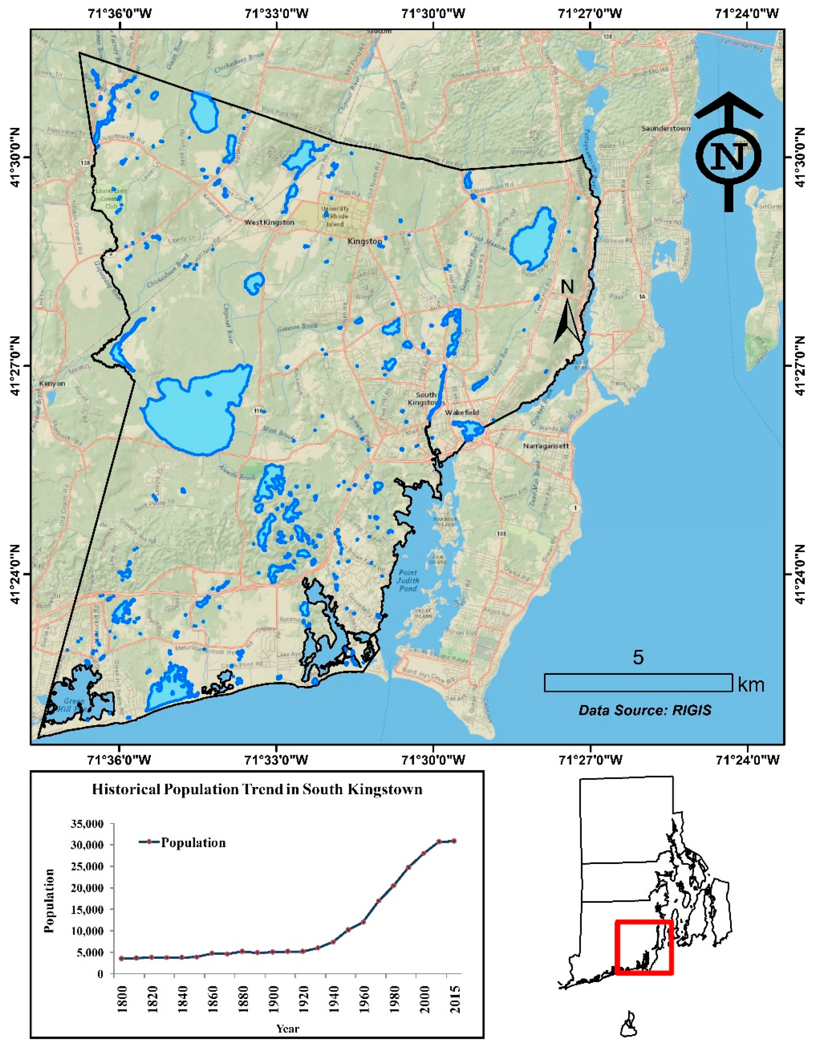
2. Study Area
3. Methodology
3.1. Surface Runoff Model
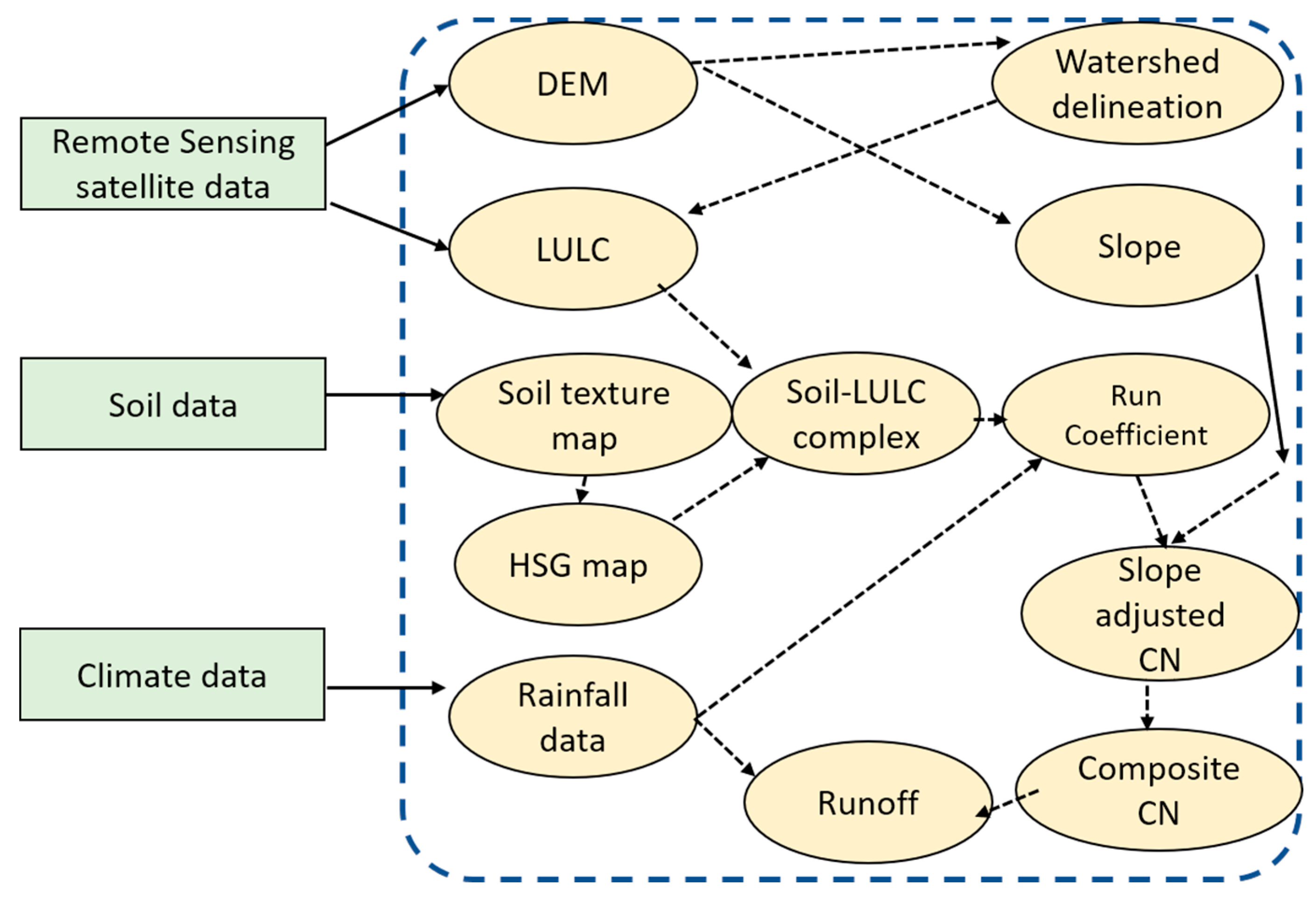
3.2. Integrated RS-GIS Approach to Surface Runoff Modeling
3.2.1. Land-Use and Land Cover Type Using Remote Sensing
3.2.2. Hydrogeological Parameter Determination Using GIS
Derivation of Soil Data
Derivation of Slope, Elevation, and Stream Order Data
Rainfall Data
3.2.3. Hydrological Modeling within GIS
4. Results and Discussion
4.1. Suburban Growth in the Study Area
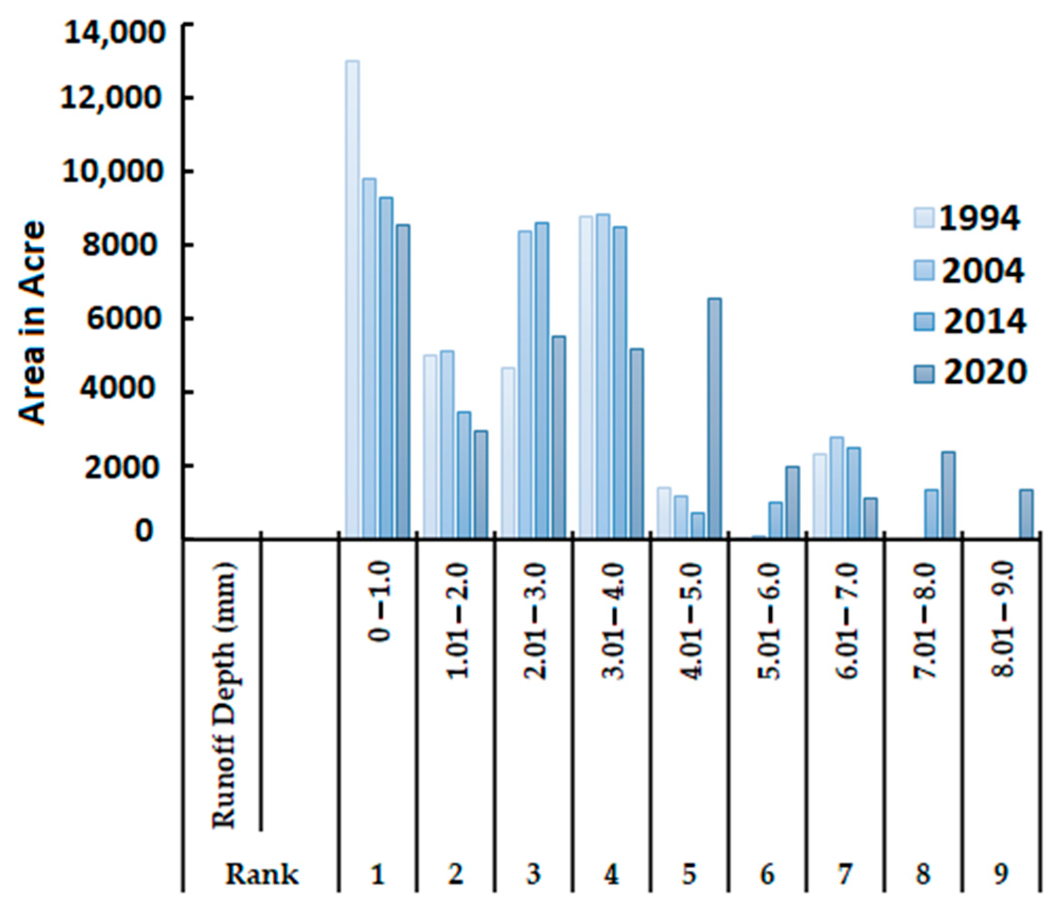
4.2. Impact of Suburban Growth on Surface Runoff
4.3. Impact of Suburban Growth on Rainfall–Runoff Relationship
5. Conclusions
Author Contributions
Funding
Institutional Review Board Statement
Informed Consent Statement
Data Availability Statement
Acknowledgments
Conflicts of Interest
References
- Grimm, N.B.; Faeth, S.H.; Golubiewski, N.E.; Redman, C.L.; Wu, J.; Bai, X.; Briggs, J.M. Global Change and the Ecology of Cities. Science 2008, 319, 756–760. [Google Scholar] [CrossRef] [PubMed] [Green Version]
- Pradhanang, S.; Jahan, K. Urban Water Security for Sustainable Cities in the Context of Climate Change; Chapter 14, Water, Climate and Sustainability; John Wiley & Sons, Inc.: Hoboken, NJ, USA, 2021; pp. 213–224. [Google Scholar] [CrossRef]
- Hegazy, I.R.; Kaloop, M.R. Monitoring urban growth and land use change detection with GIS and remote sensing techniques in Daqahlia governorate Egypt. Int. J. Sustain. Built Environ. 2015, 4, 117–124. [Google Scholar] [CrossRef] [Green Version]
- UN-HABITAT (United Nations Human Settlement Programme). The State of the African Cities 2008—A Framework for Addressing Urban Challenges in Africa. Nairobi; United Nations Human Settlements Programme, Oxford University Press: Oxford, UK, 2008. [Google Scholar]
- Sankhala, S.; Singh, B. Evaluation of urban sprawl and land use land cover change using remote sensing and GIS techniques: A case study of Jaipur City, India. J. Int. J. Emerg. Technol. Adv. Eng. 2014, 4, 66–72. [Google Scholar]
- Abustan, I.; Sulaiman, A.H.; Wahid, N.A.; Baharuddin, F. Determination of rainfall-runoff characteristics in an urban area: Sungai kerayong catchment, Kuala Lumpur. In Proceedings of the 11th International Conference on Urban Drainage, Edinburgh, UK, 31 August–5 September 2008; Available online: https://citeseerx.ist.psu.edu/viewdoc/download?doi=10.1.1.517.1745&rep=rep1&type=pdf (accessed on 11 March 2021).
- Weng, Q. Modeling urban growth effects on surface runoff with the integration of remote sensing and GIS. J. Environ. Manag. 2001, 28, 737–748. [Google Scholar] [CrossRef] [PubMed]
- Kibler, D.F. (Ed.) Urban Stormwater Hydrology; American Geophysical Union: Washington, DC, USA, 1982. [Google Scholar]
- Goudie, A. The Human Impact on the Natural Environment, 3rd ed.; The MIT Press: Cambridge, MA, USA, 1990. [Google Scholar]
- Komrad, C.P. Effect of Urban Development on Floods. U.S. Geological Survey 2003, USGS Fact Sheet FS-076-03. Available online: https://pubs.usgs.gov/fs/fs07603/pdf/fs07603.pdf (accessed on 11 March 2021).
- Rogger, M.; Agnoletti, M.; Alaoui, A.; Bathurst, J.C.; Bodner, G.; Borga, M.; Chaplot, V.; Gallart, F.; Glatzel, G.; Hall, J.; et al. Land use change impacts on floods at the catchment scale: Challenges and opportunities for future research. Water Resour. Res. 2017, 53, 5209–5219. [Google Scholar] [CrossRef] [Green Version]
- Jahan, K.; Pradhanang, S. Predicting Runoff Chloride Concentrations in Suburban Watersheds Using an Artificial Neural Network (ANN). J. Hydrol. 2020, 7, 80. [Google Scholar] [CrossRef]
- Niemczynowicz, J. Urban hydrology and water management—Present and future challenges. Urban Water 1999, 1, 1–14. [Google Scholar] [CrossRef]
- Fletcher, T.; Andrieu, H.; Hamel, P. Understanding, management and modelling of urban hydrology and its consequences for receiving waters: A state of the art. Adv. Water Resour. 2013, 51, 261–279. [Google Scholar] [CrossRef]
- Isah, T. Remote Sensing Studies on Urban Change Detections. J. Int. J. Comput. Sci. Inf. Technol. Res. 2015, 3, 62–71. Available online: www.researchpublish.com (accessed on 11 March 2021).
- Oyinloye, R.O.; Adesina, F.A. Some aspect of the growth of Ibadan and their Implications for socio-economic development. J. Ife Soc. Sci. Rev. 2006, 20, 113–120. [Google Scholar]
- McGrane, S.J. Impacts of urbanisation on hydrological and water quality dynamics, and urban water management: A review. Hydrol. Sci. J. 2016, 61, 2295–2311. [Google Scholar] [CrossRef]
- Ehlers, M.; Jadkowski, M.A.; Howard, R.R.; Brostuen, D.E. Application of SPOT data for regional grow than analysis and local planning. J. Photogramm. Eng. Remote Sens. 1990, 56, 175–180. [Google Scholar]
- Treitz, P.M.; Howard, P.J.; Gong, P. Application of satellite and GIS technologies for land-cover and land-use mapping at the rural-urban fringe: A case study. J. Photogramm. Eng. Remote Sens. 1992, 58, 439–448. [Google Scholar]
- Harris, P.M.; Ventura, S.J. The integration of geographic data with remotely sensed imagery to improve classification in an urban area. J. Photogramm. Eng. Remote Sens. 1995, 61, 993–998. [Google Scholar]
- Yeh, A.G.O.; Li, X. Urban growth management in the Pear River delta—An integrated remote sensing and GIS approach. J. ITC J. 1996, 1, 77–85. [Google Scholar]
- Yeh, A.G.O.; Li, X. An integrated remote sensing and GIS approach in the monitoring and evaluation of rapid urban growth for sustainable development in the Pearl River Delta, China. Int. Plan. Stud. 1997, 2, 193–210. [Google Scholar] [CrossRef]
- Pandey, A.; Sahu, A.K. Generation of curve number using Remote Sensing and Geographic information system. J. Geospat. World 2009. Available online: https://www.geospatialworld.net/article/generation-of-curve-number-using-remote-sensing-and-geographic-information-system/ (accessed on 11 March 2021).
- Gajbhiye, S. Estimation of Surface Runoff Using Remote Sensing and Geographical Information System. J. Sci. Technol. 2015, 8, 113–122. [Google Scholar] [CrossRef]
- Engman, E.T.; Gurney, R.J. Remote sensing in hydrology. In Remote Sensing Application Series; xiv 225; Chapman & Hall: London, UK, 1991. [Google Scholar]
- Drayton, R.S.; Wilde, B.M.; Harris, J.H.K. Geographic information system approach to distributed modeling. J. Hydrol. Process. 1992, 6, 36–368. [Google Scholar]
- Mattikalli, N.M.; Devereux, B.J.; Richards, K.S. Prediction of river discharge and surface water quality using an integrated geographic information system approach. J. Int. J. Remote Sens. 1996, 17, 683–701. [Google Scholar] [CrossRef]
- Radke, J.; Andra, S.; Al-Kofani, O.; Roysan, B. Image change detection algorithms: A systematic survey. J. IEEE Trans. Image Process. 2005, 14, 291–307. [Google Scholar] [CrossRef]
- Bhuiyan, A.E.; Witharana, C.; Liljedahl, A.K.; Jones, B.M.; Daanen, R.; Epstein, H.E.; Kent, K.; Griffin, C.G.; Agnew, A. Understanding the Effects of Optimal Combination of Spectral Bands on Deep Learning Model Predictions: A Case Study Based on Permafrost Tundra Landform Mapping Using High Resolution Multispectral Satellite Imagery. J. Imaging 2020, 6, 97. [Google Scholar] [CrossRef]
- Bhuiyan, A.E.; Witharana, C.; Liljedahl, A.K. Use of Very High Spatial Resolution Commercial Satellite Imagery and Deep Learning to Automatically Map Ice-Wedge Polygons across Tundra Vegetation Types. J. Imaging 2020, 6, 137. [Google Scholar] [CrossRef]
- Nagne, A.D.; Dhumal, R.K.; Vibhute, A.D.; Nalawade, B.D.; Kale, K.V.; Mehrotra, S.C. Advantages in Land use classification of urban areas from Hyperspectral data. Int. J. Eng. Tech. 2018, 4. Available online: http://www.ijetjournal.org (accessed on 11 March 2021).
- Witharana, C.; Bhuiyan, M.A.E.; Liljedahl, A.K. Big Imagery and high-performance computing as resources to understand changing Arctic polygonal tundra. Int. Arch. Photogramm. 2020, 44, 111–116. [Google Scholar] [CrossRef]
- Science Mission Directorate. “Wave Behaviors” NASA Science. J. Natl. Aeronaut. Space Adm. 2010. Available online: http://science.nasa.gov/ems/03_behaviors (accessed on 11 March 2021).
- Witharana, C.; Bhuiyan, M.A.E.; Liljedahl, A.K.; Kanevskiy, M.; Epstein, H.E.; Jones, B.M.; Daanen, R.; Griffin, C.G.; Kent, K.; Jones, M.K.W. Understanding the synergies of deep learning and data fusion of multispectral and panchromatic high resolution commercial satellite imagery for automated ice-wedge polygon detection. ISPRS J. Photogramm. Remote Sens. 2020, 170, 174–191. [Google Scholar] [CrossRef]
- Mohanrajan, S.N.; Loganathan, A.; Manoharan, P. Survey on Land Use/Land Cover (LU/LC) change analysis in remote sensing and GIS environment: Techniques and Challenges. Environ. Sci. Pollut. Res. 2020, 27, 29900–29926. [Google Scholar] [CrossRef] [PubMed]
- Mukherjee, S. Land use maps for conservation of ecosystems. J. Geog. Rev. India 1987, 3, 23–28. [Google Scholar]
- Sharma, S.K.; Gajbhiye, S.; Nema, R.K.; Tignath, S. Assessing vulnerability to soil erosion of a watershed of tons River basin in Madhya Pradesh using Remote sensing and GIS. J. Int. J. Environ Res Dev 2014, 4, 153–164. [Google Scholar]
- Berry, J.K.; Sailor, J.K. Use of a Geographic Information System for storm runoff prediction from small urban watersheds. J. Environ. Manag. 1987, 11, 21–27. [Google Scholar] [CrossRef]
- Dongquan, Z.; Jining, C.; Haozheng, W.; Qingyuan, T.; Shangbing, C.; Zheng, S. GIS-based urban rainfall-runoff modeling using an automatic catchment-discretization approach: A case study in Macau. Environ. Earth Sci. 2009, 59, 465–472. [Google Scholar] [CrossRef]
- Mishra, S.K.; Pandey, A.; Singh, V.P. Special Issue on Soil Conservation Service Curve Number (SCS-CN) Methodology. J. Hydrol. Eng. 2012, 17, 1157. [Google Scholar] [CrossRef]
- Singh, P.K.; Mishra, S.K.; Berndtsson, R.; Jain, M.K.; Pandey, R.P. Development of a Modified SMA Based MSCS-CN Model for Runoff Estimation. Water Resour. Manag. 2015, 29, 4111–4127. [Google Scholar] [CrossRef]
- Vojtek, M.; Vojteková, J. GIS-based Approach to Estimate Surface Runoff in Small Catchments: A Case Study. Quaest. Geogr. 2016, 35, 97–116. [Google Scholar] [CrossRef] [Green Version]
- Soulis, K.X.; Valiantzas, J.D. SCS-CN parameter determination using rainfall-runoff data in heterogeneous watersheds. The two-CN system approach. J. Hydrol. Earth Syst. Sci. Discuss. 2011, 8, 8963–9004. [Google Scholar]
- Mishra, S.K.; Singh, V.P. Long-term hydrological simulation based on the Soil Conservation Service curve number. Hydrol. Process. 2004, 18, 1291–1313. [Google Scholar] [CrossRef]
- Soulis, K.X.; Dercas, N. Development of a GIS-based spatially distributed continuous hydrological model and its first application. J. Water Int. 2007, 32, 177–192. [Google Scholar] [CrossRef]
- Zhan, X.Y.; Huang, M.L. ArcCN-Runoff: An ArcGIS tool for generating curve number and runoff maps. J. Environ. Model. Softw. 2004, 19, 875–879. [Google Scholar] [CrossRef]
- Moretti, G.; Montanari, A. Inferring the flood frequency distribution for an ungauged basin using a spatially distributed rainfall-runoff model. Hydrol. Earth Syst. Sci. 2008, 12, 1141–1152. [Google Scholar] [CrossRef] [Green Version]
- Adornado, H.A.; Yoshida, M. GIS-based watershed analysis and surface runoff estimation using curve number (C.N.) value. J. Environ. Hydrol. 2010, 18, 1–10. [Google Scholar]
- Wilcox, B.P.; Rawls, W.J.; Brakensiek, D.L.; Wight, J.R. Predicting runoff from Rangeland Catchments: A comparison of two models. Water Resour. Res. 1990, 26, 2401–2410. [Google Scholar] [CrossRef]
- Holman, I.P.; Hollis, J.M.; Bramley, M.E.; Thompson, T.R.E. The contribution of soil structural degradation to catchment flooding: A preliminary investigation of the 2000 floods in England and Wales. Hydrol. Earth Syst. Sci. 2003, 7, 755–766. [Google Scholar] [CrossRef] [Green Version]
- Romero, P.; Castro, G.; Gomez, J.A.; Fereres, E. Curve number values fo olive orchards under different soil management. J. Soil Sci. Soc. Am. J. 2007, 71, 1758–1769. [Google Scholar] [CrossRef]
- Tedela, N.H.; McCutcheon, S.C.; Rasmussenn, T.C.; Hawkins, R.H.; Swank, W.T.; Campbell, J.L.; Adams, M.B.; Jackson, R.; Tollner, E.W. Runoff curve numbers for 10 small forested watersheds in the mountains of the eastern united states. J. Hydrol. Eng. 2012, 17, 1188–1198. [Google Scholar] [CrossRef] [Green Version]
- Nagarajan, M.; Basil, G. Remote sensing- and GIS-based runoff modeling with the effect of land-use changes (a case study of Cochin corporation). Nat. Hazards 2014, 73, 2023–2039. [Google Scholar] [CrossRef]
- Pandit, A.; Gopalakrishnan, G. Estimtion of annual storm runoff coefficients by continuous simulation. J. Irrig. Drain. Eng. 1996, 122, 211–220. [Google Scholar] [CrossRef]
- USGS. Elevation of the March-April 2010 Flood High Water in Selected River Reaches in Rhode Island by Phillip, J. Zarriello and Gardener, C. Bent; U.S. Department of the Interior. U.S. Geological Survey: Reston, VA, USA, 2011. Available online: https://pubs.usgs.gov/of/2011/1029/pdf/ofr2011-1029-508.pdf (accessed on 11 March 2021).
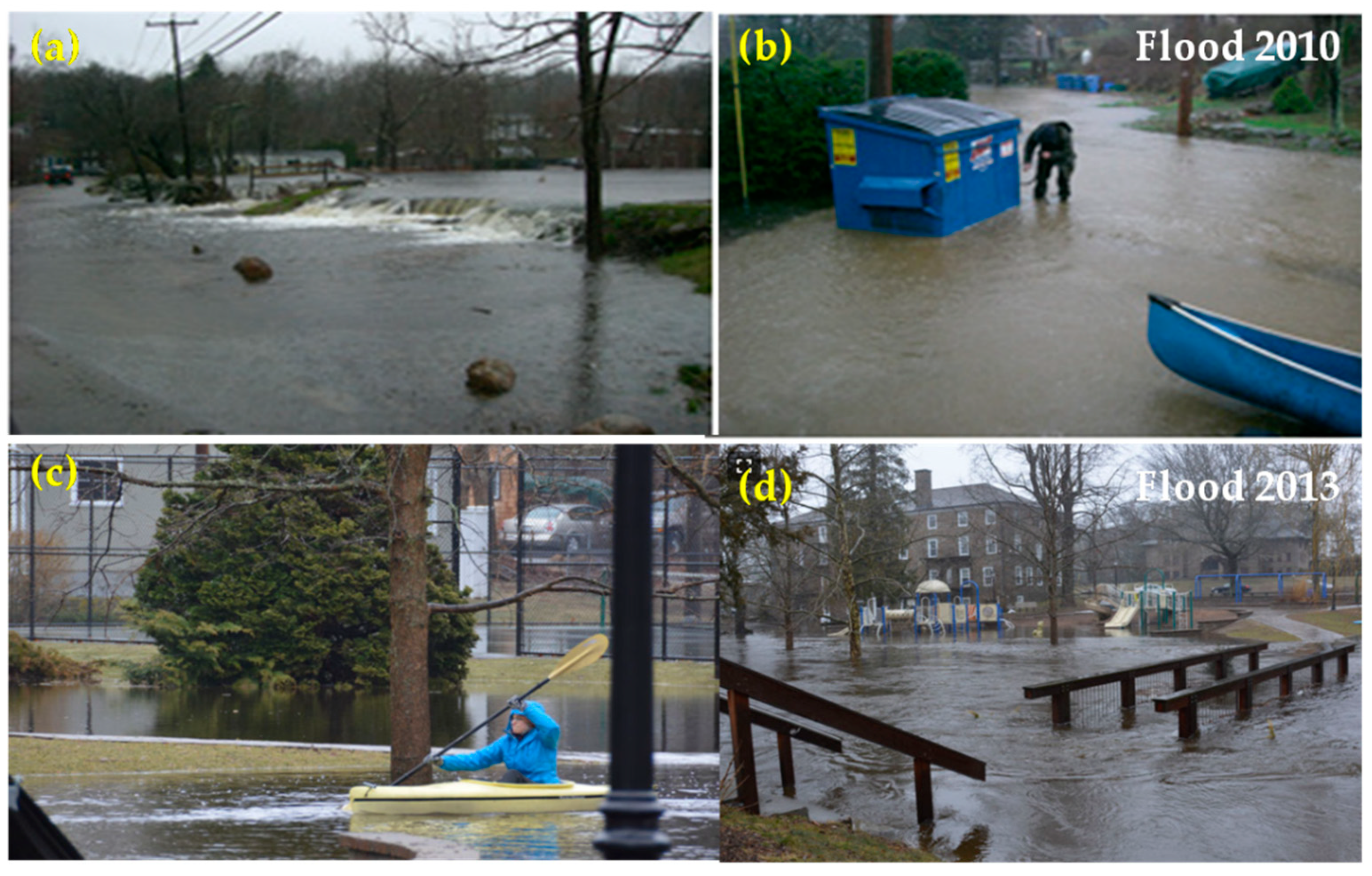
- Kenyon Grist Mill. Flood 2010: Photo Documentary (Before, During, and After). All Content Copyright—Official Website of Kenyon Grist Mill LLC 21 Glen Rock Road/P.O. Box 221 West Kingston, RI 02892. 2013. Available online: https://www.kenyonsgristmill.com/flood2010.html (accessed on 11 March 2021).
- The Independent. Towns, Reesidents Close to Recoverig From Historic Flood by Chris Church. 2011. Available online: https://www.independentri.com/local/article_71f7559f-a7ec-537d-b380-80ac5e5c3ddb.html (accessed on 11 March 2021).
- SRI. A Look Back at the Flood of the Century. Southern Rhode Island Newspaper. 2011. Available online: https://www.ricentral.com/a-look-back-at-the-flood-of-the-century/article_c8e44c9d-a7f9-59f8-ac2b-f345b5f0e0a9.html (accessed on 11 March 2021).
- Gorman, G. Rhode Island Flood Zones-South KingstownRI Real Estate Has Them too. Rhode Island Coastal Real Estate. 2012. Available online: https://www.rihousehunt.com/ri-blog/rhode-island-flood-zones-south-kingstown-ri-real-estate-has-them-too/?doing_wp_cron=1614615852.4240589141845703125000 (accessed on 11 March 2021).
- The Independent. Heavy Rains Brings Flooding, Road Closures. Reporter Stephen Greenwell. 2014. Available online: https://www.independentri.com/independents/south_county/article_35880c91-006d-5e2b-b32b-af311135fe9e.html (accessed on 11 March 2021).
- Patch the Community Corner. Flash Flood Watch in Narragensett and South Kingstown by Erin Tiernan. Community Corner. 2013. Available online: https://patch.com/rhode-island/narragansett/flash-flood-watch-in-narragansett-and-south-kingstown (accessed on 11 March 2021).
- ECO RI News. Rising Waters Threaten Region’s Cultural Treasures. ECO RI News. 2015. Available online: https://www.ecori.org/climate-change/2015/1/5/rising-waters-threaten-regions-culture (accessed on 11 March 2021).
- USDA. Economic Research Service Using Data from U.S. Census Bureau. 2013. Available online: https://www.ers.usda.gov/data-products/ (accessed on 11 March 2021).
- U.S. Climate Data. U.S. Climate Data 2021|Version 3.0|by Your Weather Service. 2019. Available online: https://www.usclimatedata.com/ (accessed on 11 March 2021).
- South Kingstown Source of Water Assessment (SKSWA), University of Rhode Island Cooperative Extension. 2003. Available online: http://cels.uri.edu/rinemo/assesments/sk_source_water_assesment.pdf (accessed on 11 March 2021).
- USGS Earth Explorer Landsat Archive (1980–2019). Available online: https://earthexplorer.usgs.gov (accessed on 10 February 2019).
- Jensen, J.R. Introductory Digital Image Processing: A Remote Sensing Perspective, 2nd ed.; Prentice-Hall: Hoboken, NJ, USA, 1996. [Google Scholar]
- USDA—Soil Conservation Service. National Engineering Handbook; Sec. 4. Hydrology; USDA: Washington, DC, USA, 1972.
- Rango, A.; Feldman, A.; George, T.S.; Ragan, R.M. Effective use of landsat data in hydrologic models. JAWRA J. Am. Water Resour. Assoc. 1983, 19, 165–174. [Google Scholar] [CrossRef]
- Camps-Valls, G.; Tuia, D.; Gómez-Chova, L.; Jiménez, S.; Malo, J. Remote Sensing Image Processing. Synth. Lect. Image Video Multimedia Process. 2011, 5, 1–192. [Google Scholar] [CrossRef]
- Hütt, C.; Koppe, W.; Miao, Y.; Bareth, G. Best Accuracy Land Use/Land Cover (LULC) Classification to Derive Crop Types Using Multitemporal, Multisensor, and Multi-Polarization SAR Satellite Images. Remote Sens. 2016, 8, 684. [Google Scholar] [CrossRef] [Green Version]
- Samaniego, L.; Schulz, K. Supervised Classification of Agricultural Land Cover Using a Modified k-NN Technique (MNN) and Landsat Remote Sensing Imagery. Remote Sens. 2009, 1, 875–895. [Google Scholar] [CrossRef] [Green Version]
- Anderson, J.R.; Hardy, E.E.; Roach, J.T.; Witmer, R.E. A Land Use and Land Cover Classification for Use with Remote Sensor Data; (USGS Professional Paper 964); Government Printing Oce: Washington, DC, USA, 1976. [CrossRef] [Green Version]
- USDA. Urban Hydrology for Small Watershed TR-55. In 210-VI-TR-55, 2nd ed.; USDA: Washington, DC, USA, 1986. [Google Scholar]
- Daly, C. Guidelines for assessing the suitability of spatial climate data sets. Int. J. Clim. 2006, 26, 707–721. [Google Scholar] [CrossRef]
- Bhuiyan, M.A.E.; Yang, F.; Biswas, N.K.; Rahat, S.H.; Neelam, T.J. Machine Learning-Based Error Modeling to Improve GPM IMERG Precipitation Product over the Brahmaputra River Basin. Forecasting 2020, 2, 14. [Google Scholar] [CrossRef]
- Bhuiyan, M.A.; Nikolopoulos, E.I.; Anagnostou, E.N. Machine learning–based blending of satellite and reanalysis precipitation datasets: A multiregional tropical complex terrain evaluation. J. Hydrometeorol. 2019, 20, 2147–2161. [Google Scholar] [CrossRef]
- Bhuiyan, M.A.E.; Nikolopoulos, E.I.; Anagnostou, E.N.; Quintana-Seguí, P.; Barella-Ortiz, A. A nonparametric statistical technique for combining global precipitation datasets: Development and hydrological evaluation over the Iberian Peninsula. Hydrol. Earth Syst. Sci. 2018, 22, 1371–1389. [Google Scholar] [CrossRef] [Green Version]
- Journel, A.G.; Huijbregts, C.J. Mining Geostatistics; Academic Press: Cambridge, MA, USA, 1978; 600p. [Google Scholar]


| S.No. | Date of Images | Satellite | Sensors | Resolution (m) | Bands | Thermal Band |
|---|---|---|---|---|---|---|
| 1. | 19 September 1994 | LANDSAT-5 | TM | 30 | 7 | 6 |
| 2. | 14 September 2004 | LANDSAT-5 | TM | 30 | 7 | 6 |
| 3. | 18 September 2014 | LANDSAT-7 | ETM | 30 | 8 | 6 |
| 4. | 9 August 2020 | LANDSAT-8 | OLI | 30 | 11 | 10 and 11 |
| Land Type | A | B | C | D |
|---|---|---|---|---|
| Agricultural Land | 64 | 75 | 82 | 85 |
| Commercial | 89 | 92 | 94 | 95 |
| Forest | 30 | 55 | 70 | 77 |
| Grass/Pasture | 39 | 61 | 74 | 80 |
| Residential | 60 | 74 | 83 | 87 |
| Industrial | 81 | 88 | 91 | 93 |
| Open Space | 49 | 69 | 79 | 84 |
| Parking and paved spaces | 98 | 98 | 98 | 98 |
| Water/Wetlands | 0 | 0 | 0 | 0 |
| Land Type | Calculated Area (Acre) | Change Detection of the Area | ||
|---|---|---|---|---|
| 1994 | 2020 | Area (Acre) | % | |
| Urban | 9569 | 16,133 | 6564 | 68.6 |
| Agriculture | 2684 | 2814 | 130 | 4.8 |
| Forest | 18,440 | 16,934 | −1506 | −8.2 |
| Grass/Pasture | 6662 | 710 | −5952 | −89.3 |
Publisher’s Note: MDPI stays neutral with regard to jurisdictional claims in published maps and institutional affiliations. |
© 2021 by the authors. Licensee MDPI, Basel, Switzerland. This article is an open access article distributed under the terms and conditions of the Creative Commons Attribution (CC BY) license (https://creativecommons.org/licenses/by/4.0/).
Share and Cite
Jahan, K.; Pradhanang, S.M.; Bhuiyan, M.A.E. Surface Runoff Responses to Suburban Growth: An Integration of Remote Sensing, GIS, and Curve Number. Land 2021, 10, 452. https://doi.org/10.3390/land10050452
Jahan K, Pradhanang SM, Bhuiyan MAE. Surface Runoff Responses to Suburban Growth: An Integration of Remote Sensing, GIS, and Curve Number. Land. 2021; 10(5):452. https://doi.org/10.3390/land10050452
Chicago/Turabian StyleJahan, Khurshid, Soni M. Pradhanang, and Md Abul Ehsan Bhuiyan. 2021. "Surface Runoff Responses to Suburban Growth: An Integration of Remote Sensing, GIS, and Curve Number" Land 10, no. 5: 452. https://doi.org/10.3390/land10050452
APA StyleJahan, K., Pradhanang, S. M., & Bhuiyan, M. A. E. (2021). Surface Runoff Responses to Suburban Growth: An Integration of Remote Sensing, GIS, and Curve Number. Land, 10(5), 452. https://doi.org/10.3390/land10050452