
Analysis of Factors Influencing the Urban Carrying Capacity of the Shanghai Metropolis Based on a Multiscale Geographically Weighted Regression (MGWR) Model


Abstract
:1. Introduction
2. Study Area and Data
2.1. Study Area
2.2. Influencing Factors and Data Processing
3. Methods
4. Results
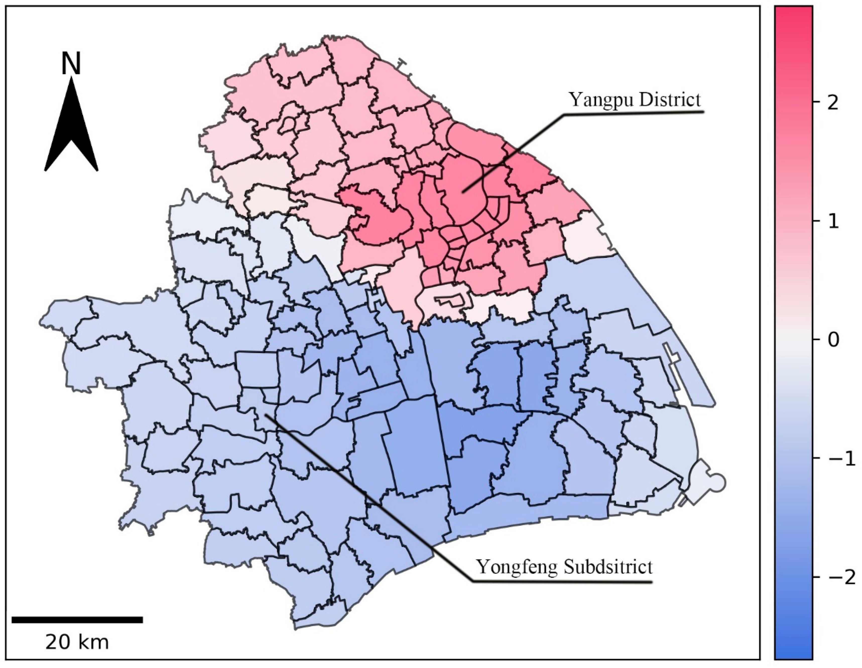
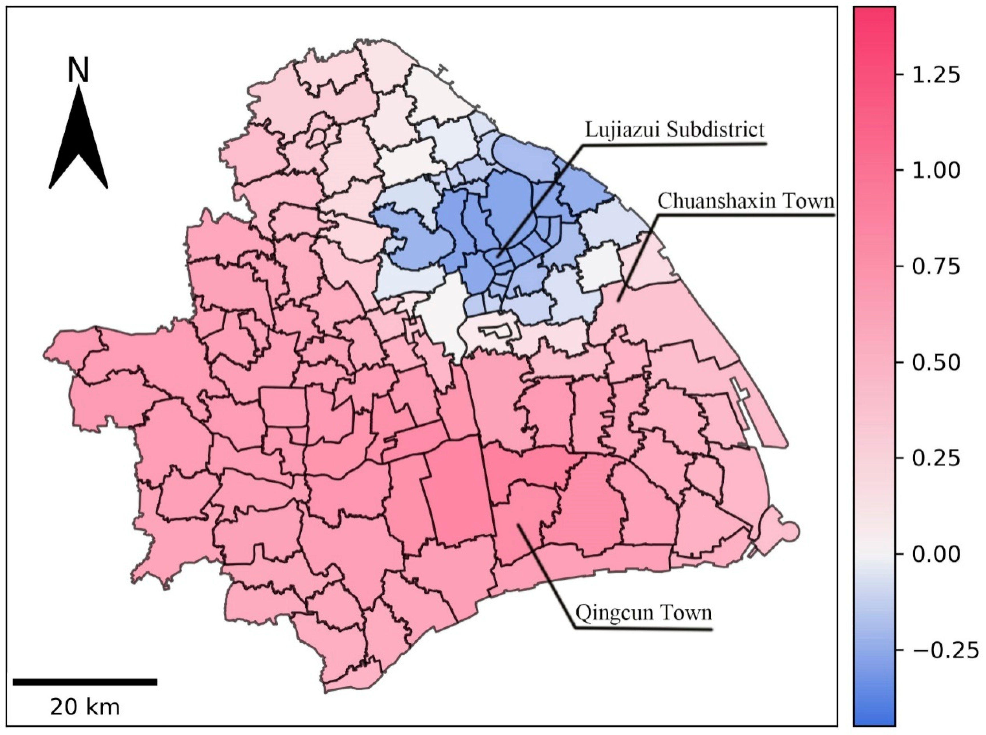
4.1. Analysis of the Influence of Location Factors
4.2. Influence Analysis of the Average Floor Area Ratio
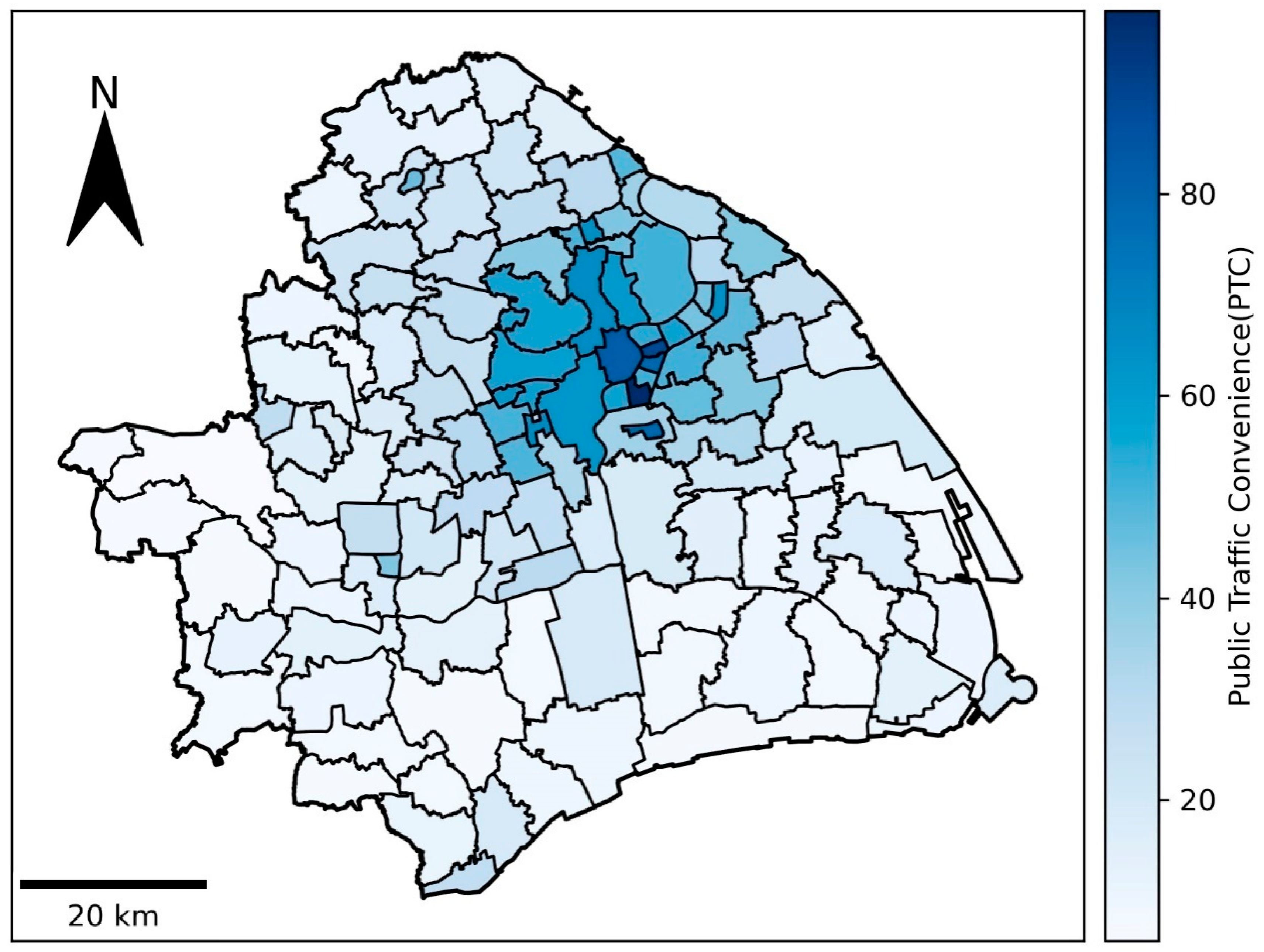
4.3. Impact Analysis of Public Transportation Convenience
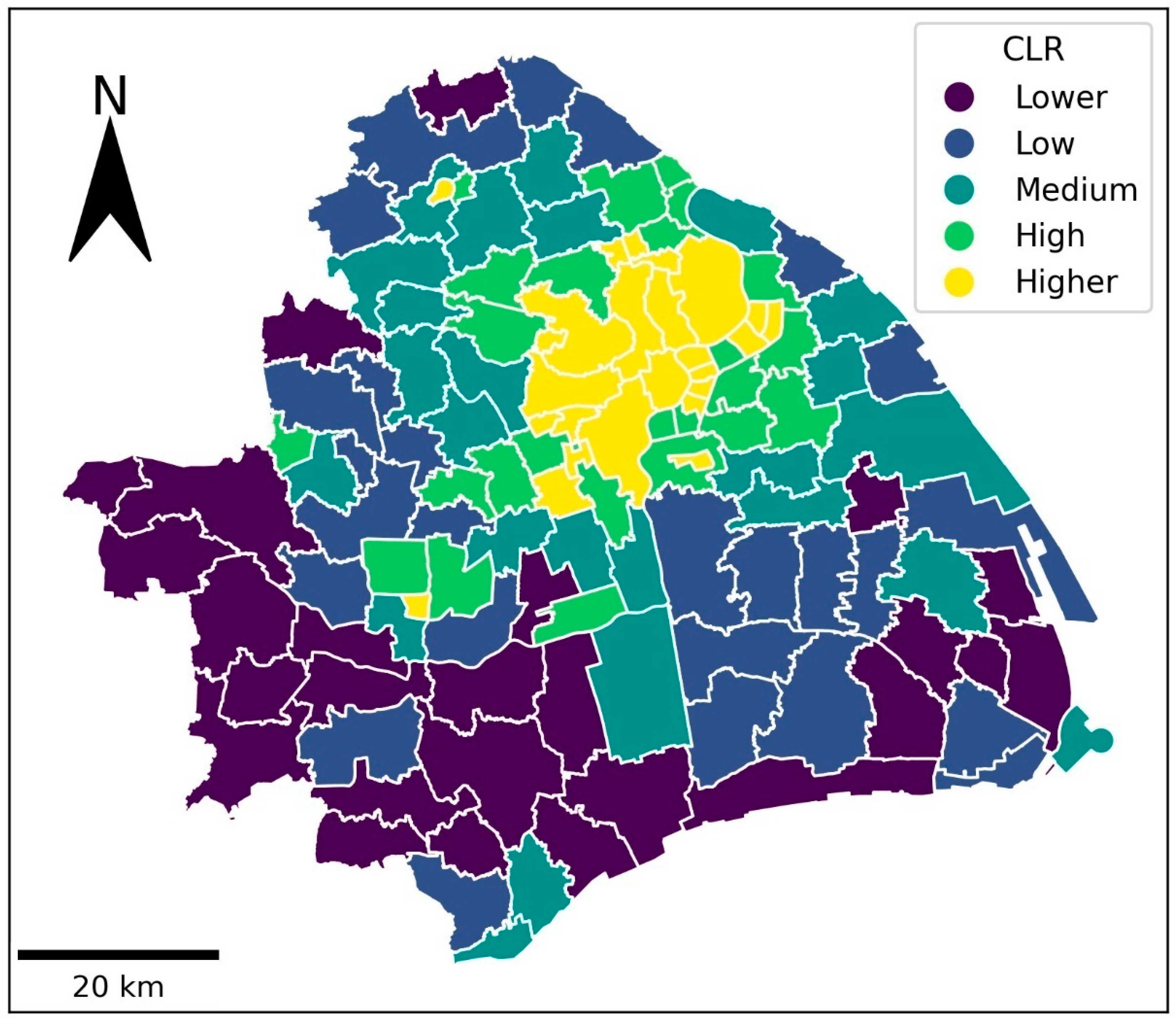
4.4. Impact Analysis of Residents’Consumption Level
4.5. Influence Analysis of High-tech Enterprise Density
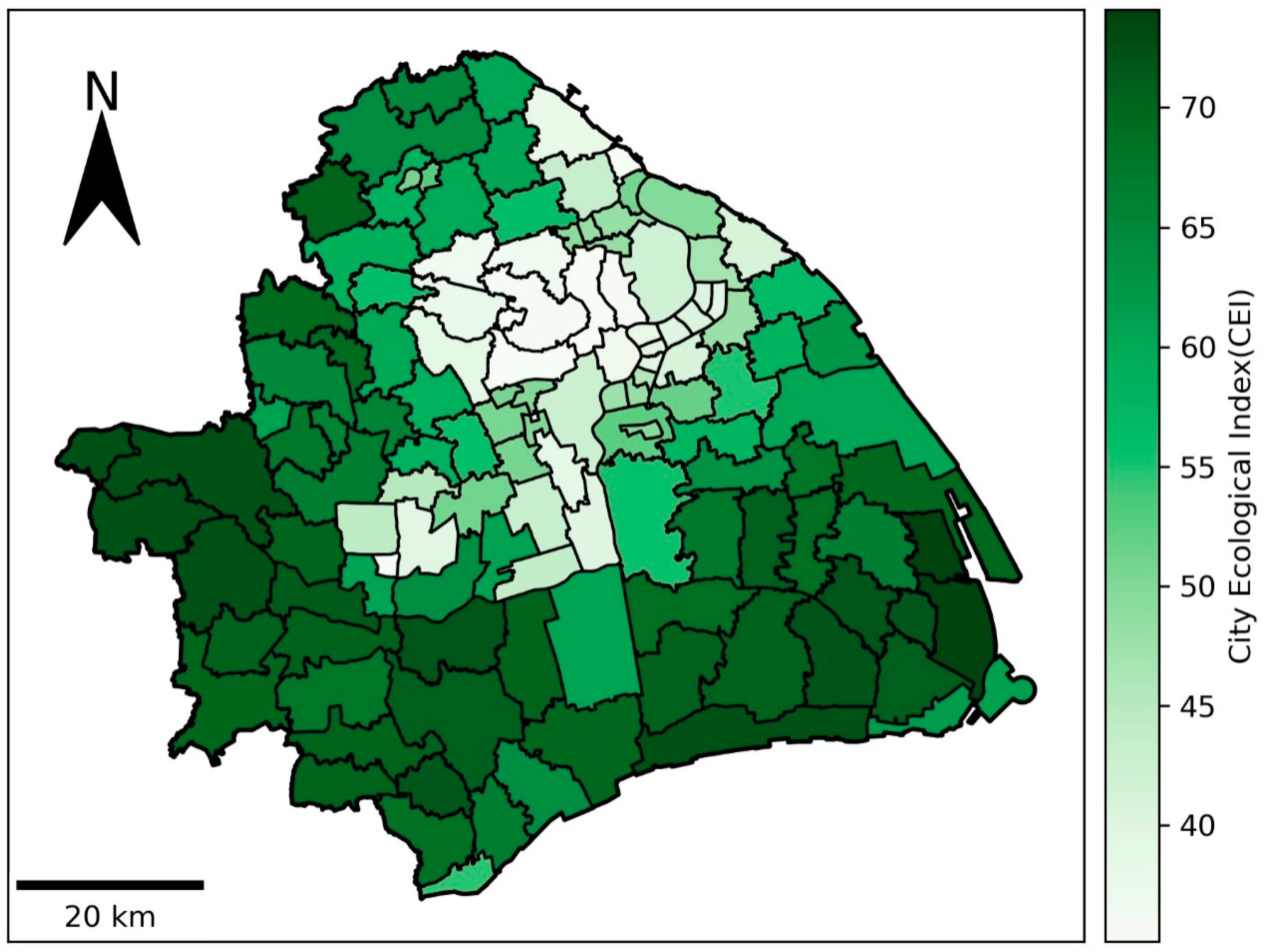
4.6. Impact Analysis of the Urban Ecological Environment Status Index
5. Discussion
6. Conclusions
Author Contributions
Funding
Institutional Review Board Statement
Informed Consent Statement
Data Availability Statement
Conflicts of Interest
References
- Sun, M.; Wang, J.; He, K. Analysis on the urban land resources carrying capacity during urbanization: A case study of Chinese YRD. Appl. Geogr. 2020, 116, 102170. [Google Scholar] [CrossRef]
- Shao, Q.; Liu, X.; Zhao, W. An alternative method for analyzing dimensional interactions of urban carrying capacity: Case study of Guangdong-Hong Kong-Macao Greater Bay Area. J. Environ. Manag. 2020, 273, 111064. [Google Scholar] [CrossRef]
- Liu, Z.; Ren, Y.; Shen, L.; Liao, X.; Wei, X.; Wang, J. Analysis on the effectiveness of indicators for evaluating urban carrying capacity: A popularity-suitability perspective. J. Clean. Prod. 2020, 246, 119019. [Google Scholar] [CrossRef]
- Chen, W.; Yi, C. Research on water resources bearing capacity of Wuhan based on multivariate linear regression model. J. Henan Polytech. Univ. Nat. Sci. 2017, 36, 75–79. (In Chinese) [Google Scholar]
- Shen, W.; Lu, F.; Qin, Y.; Xie, Z.; Li, Y. Analysis of temporal-spatial patterns and influencing factors of urban ecosystem carrying capacity in urban agglomeration in the middle reaches of the Yangtze River. Acta Ecol. Sin. 2019, 39, 3937–3951. (In Chinese) [Google Scholar]
- Lam, C.; Souza, P.C.L. Estimation and selection of spatial weight matrix in a spatial lag model. J. Bus. Econ. Stat. 2020, 38, 693–710. [Google Scholar] [CrossRef]
- Gao, C.; Feng, Y.; Tong, X.; Lei, Z.; Chen, S.; Zhai, S. Modeling urban growth using spatially heterogeneous cellular automata models: Comparison of spatial lag, spatial error and GWR. Comput. Environ. Urban Syst. 2020, 81, 101459. [Google Scholar] [CrossRef]
- Zhou, W.; Zhao, Y.; Ning, X. Analysis on the influencing factors of manufacturing structure change and spatial agglomeration in Beijing-Tianjin-Hebei urban agglomeration. Sci. Geogr. Sin. 2020, 40, 1921–1929. (In Chinese) [Google Scholar]
- Kolomak, E.A. Estimation of the spatial connectivity of the economic activity of Russian regions. Reg. Res. Russ. 2020, 10, 301–307. [Google Scholar] [CrossRef]
- Sun, F.; Matthews, S.A.; Yang, T.C.; Hu, M.-H. A spatial analysis of the COVID-19 period prevalence in US counties through June 28, 2020: Where geography matters? Ann. Epidemiol. 2020, 52, 54–59. [Google Scholar] [CrossRef]
- Guliyev, H. Determining the spatial effects of COVID-19 using the spatial panel data model. Spat. Stat. 2020, 38, 100443. [Google Scholar] [CrossRef]
- Liu, Y.; Chang, Y.; Li, F. Application of spatial error model to spatial distribution of forest carbon storage in Heilongjiang Province. Chin. J. Appl. Ecol. 2014, 25, 2779–2786. (In Chinese) [Google Scholar]
- Zhu, L.; He, Y. A Study of the dynamic evolution and influencing factors of cities’ bearing capacity in the Yangtze River economic belt—Based on the perspective of spatial spillover effect. J. China Exec. Leadersh. Acad. Jinggangshan 2020, 77, 60–69. (In Chinese) [Google Scholar]
- Pi, Q.; Wang, X.; Zhang, L. Study on the influencing factors of urban energy carrying capacity based on SD model. Stat. Decis. Mak. 2016, 32, 109–112. (In Chinese) [Google Scholar]
- Goodchild, M.F. Models of Scale and Scales of Modelling. In Modelling Scale in Geographical Information Science; Tate, N.J., Atkinson, P.M., Eds.; John Wiley and Sons: New York, NY, USA, 2001. [Google Scholar]
- Sheppard, E.; McMaster, R.B. (Eds.) Scale and Geographic Inquiry: Nature, Society and Method; Blackwell Publishing Ltd.: Malden, MA, USA, 2004. [Google Scholar]
- Fotheringham, A.S.; Yang, W.; Kang, W. Multiscale Geographically Weighted Regression (MGWR). Ann. Am. Assoc. Geogr. 2017, 107, 1247–1265. [Google Scholar] [CrossRef]
- Guo, J.; Sun, B.; Qin, Z.; Wong, S.W.; Wong, M.S.; Yeung, C.W.; Shen, Q. A Study of Plot ratio/Building Height Restrictions in High Density Cities Using 3D Spatial Analysis Technology: A Case in Hong Kong. Habitat Int. 2017, 65, 13–31. [Google Scholar] [CrossRef] [Green Version]
- Oh, K.; Jeong, Y.; Lee, D.; Lee, W.; Choi, J. Determining Development Density Using the Urban Carrying Capacity Assessment System. Landsc. Urban Plan. 2005, 73, 1–15. [Google Scholar] [CrossRef]
- Meng, C.; Du, X.; Ren, Y.; Shen, L.; Cheng, G.; Wang, J. Sustainable Urban Development: An Examination of Literature Evolution on Urban Carrying Capacity in the Chinese Context. J. Clean. Prod. 2020, 277, 122802. [Google Scholar] [CrossRef]
- Wei, Y.; Huang, C.; Li, J.; Xie, L. An Evaluation Model for Urban Carrying Capacity: A Case Study of China’s Mega-Cities. Habitat Int. 2016, 53, 87–96. [Google Scholar] [CrossRef]
- Zhou, Z. An Excellent Global City: National Mission and Ambition for Shanghai; Gezhi Publishing House, Shanghai People’s Publishing House: Shangai, China, 2019. (In Chinese) [Google Scholar]
- Fu, J.; Li, Y.; Xu, C. The evolution process and limiting factors of urban comprehensive carrying capacity. Urban Dev. Stud. 2014, 21, 117–122. (In Chinese) [Google Scholar]
- Ferreira, J.J.M.; Fernandes, C.I.; Raposo, M.L. The effects of location on firm innovation capacity. J. Knowl. Econ. 2017, 8, 77–96. [Google Scholar] [CrossRef]
- Kato, H. How does the location of urban facilities affect the forecasted population change in the Osaka metropolitan fringe area? Sustainability 2021, 13, 110. [Google Scholar] [CrossRef]
- Wang, J.-X.; Feng, B.; Hu, L.-S.; Tang, Y.-Q.; Yan, X.-X.; Wang, H.-M.; Liu, J.-B. Application of Geo-Environmental Capacity of Ground Buildings in Urban Planning. Environ. Earth Sci. 2013, 69, 93–102. [Google Scholar] [CrossRef]
- Shi, Y.; Wang, H.; Yin, C. Evaluation method of urban land population carrying capacity based on GIS-A case of Shanghai, China. Comput. Environ. Urban Syst. 2013, 39, 27–38. [Google Scholar] [CrossRef]
- Jennie, M. Ecological footprints and lifestyle archetypes: Exploring dimensions of consumption and the transformation needed to achieve urban sustainability. Sustainability 2015, 7, 4747–4763. [Google Scholar]
- Zhu, T.; Wang, J.; Kim, H. Research on enhancing talent gathering capacity in Shaoxing city: A comparative analysis based on relevant prefecture-level cities in the Yangtze River Delta. J. Asia-Pac. Stud. 2020, 27, 265–279. [Google Scholar]
- Miharja, M.; Sjafruddin, A.H. Urban Development Control Based on Transportation Carrying Capacity; IOP Conference Series: Earth and Environmental Science; IOP Publishing: Bristol, UK, 2017; Volume 70, p. 012019. [Google Scholar]
- Zhao, J.Z.; Lou, S.; Fonseca, C.; Feiock, R.; Shen, R. Explaining Transit Expenses in US Urbanised Areas: Urban Scale, Spatial Form and Fiscal Capacity. Urban Stud. 2021, 58, 280–296. [Google Scholar] [CrossRef]
- Elizaveta, D.; Olga, T.; Ilin, I. Analysis of the influence of external environmental factors on the development of high-tech enterprises. MATEC Web Conf. 2018, 170, 01027. [Google Scholar]
- Tsou, J.; Gao, Y.; Zhang, Y.; Genyun, S.; Ren, J.; Li, Y. Evaluating Urban Land Carrying Capacity Based on the Ecological Sensitivity Analysis: A Case Study in Hangzhou, China. Remote. Sens. 2017, 9, 529. [Google Scholar] [CrossRef] [Green Version]
- Zhang, Y.; Wei, Y.; Zhang, J. Overpopulation and Urban Sustainable development—population Carrying Capacity in Shanghai Based on Probability-Satisfaction Evaluation Method. Environ. Dev. Sustain. 2021, 23, 3318–3337. [Google Scholar] [CrossRef]
- Galli, A.; Iha, K.; Pires, S.M.; Mancini, M.S.; Alves, A.A.; Zokai, G.; Lin, D.; Murthy, A.; Wackernagel, M. Assessing the Ecological Footprint and Biocapacity of Portuguese Cities: Critical Results for Environmental Awareness and Local Management. Cities 2020, 96, 102442. [Google Scholar] [CrossRef]
- Shi, Y.; Shi, S.; Wang, H. Reconsideration of the methodology for estimation of land population carrying capacity in Shanghai metropolis. Sci. Total. Environ. 2019, 652, 367–381. [Google Scholar] [CrossRef] [PubMed]
- Shi, Y.; Wang, H.; Yin, C.; Wu, J.; Hang, T. Research on Estimation Methods for the Carrying Capacity of Resources and Environment in Shanghai Metropolitan Area; Building Industry Press: Beijing, China, 2015. (In Chinese) [Google Scholar]
- Shen, T.; Yu, H.; Zhou, L.; Gu, H. Influence mechanism of second-hand housing price in Beijing: A study based on multi-scale geographically weighted regression model. Econ. Geogr. 2020, 40, 75–83. (In Chinese) [Google Scholar]
- Xian, B.; Chen, X. Discussion on the determination method of reasonable floor area ratio. Planners 2008, 24, 60–65. (In Chinese) [Google Scholar]
- Zhang, L.; Lu, Y. Regional accessibility evaluation based on land transport network: A case study of the Yangtze River Delta. Acta Geogr. Sin. 2006, 61, 1235–1246. (In Chinese) [Google Scholar]
- Wu, Y.; Chen, Z. Spatial correlation and regional convergence analysis of household consumption level. World Econ. Pap. 2009, 29, 76–89. (In Chinese) [Google Scholar]
- Technical Ministry of Ecology and Environment of the PRC. Technical Specification for Evaluation of Ecological Environment conditions (HJ 192-2015). Available online: http://www.mee.gov.cn/ywgz/fgbz/bz/bzwb/stzl/201503/t20150324_298011.shtml (accessed on 9 August 2019). (In Chinese)
- Brunsdon, C.; Fotheringham, A.S.; Charlton, M.E. Geographically Weighted Regression: A Method for Exploring Spatial Nonstationarity. Geogr. Anal. 1996, 28, 281–298. [Google Scholar] [CrossRef]
- Huang, Y.; Zhao, C.; Song, X.; Chen, J.; Li, Z. A semi-parametric geographically weighted regression (S-GWR) approach for modelling spatial distribution of population. Ecological. Indicators 2018, 85, 1022–1029. [Google Scholar] [CrossRef]
- Chen, Y.; Waters, E.; Green, J. Geospatial analysis of childhood pertussis in Victoria, 1993–1997. Aust. N. Z. J. Public Health 2002, 26, 456–461. [Google Scholar] [CrossRef] [Green Version]
- Fotheringham, A.S.; Crespo, R.; Yao, J. Geographical and temporal weighted regression (GTWR). Geogr. Anal. 2015, 47, 431–452. [Google Scholar] [CrossRef] [Green Version]


| Independent Variables | Abbreviations | Main Authors |
|---|---|---|
| Location | Location | Ferreira et al., 2017; Kato, 2021 |
| Average floor area ratio | AFAR | Wang et al., 2013; Shi et al., 2013 |
| Consumption level of residents | CLR | Jennie, 2015 |
| Living service level | LSL | Zhu et al., 2020 |
| Public traffic convenience | PTC | Miharja and Sjafruddin, 2017; Zhao et al., 2021 |
| High-tech enterprise density | HED | Elizaveta et al., 2018 |
| Abundance of natural resources | ANR | Tsou et al., 2017 |
| Level of science and technology | LST | Zhang et al., 2020 |
| City ecological index | CEI | Galli et al., 2020 |
| Policies and regulations | PR | Oh et al., 2005 |
| Classification | Indicators | Weight | Normalized Coefficient Reference Value | Type |
|---|---|---|---|---|
| Environmental quality (B1) | Air quality compliance rate (H1) | 0.64 | 100 (A1) | + |
| Water quality up to standard (H2) | 0.36 | 100 (A2) | + | |
| Pollution load (B2) | Nitrogen oxide emission intensity (H3) | 0.5 | 0.1398466842 (A3) | - |
| Sulphur dioxide emission intensity (H4) | 0.5 | 0.0673890063 (A4) | - | |
| Ecological construction (B3) | Proportion of ecological land (H5) | 0.5 | 100 (A5) | + |
| Green space coverage (H6) | 0.5 | 171.02787754 (A6) | + |
| Predictive Variable | SEM Parameter Estimation | |
|---|---|---|
| Range of Coefficient | Mean | |
| Intercept term (location in MGWR) | −2.695 to 2.805 | −0.05 |
| Average floor area ratio (AFAR) | −0.449 to 1.426 | 0.52 |
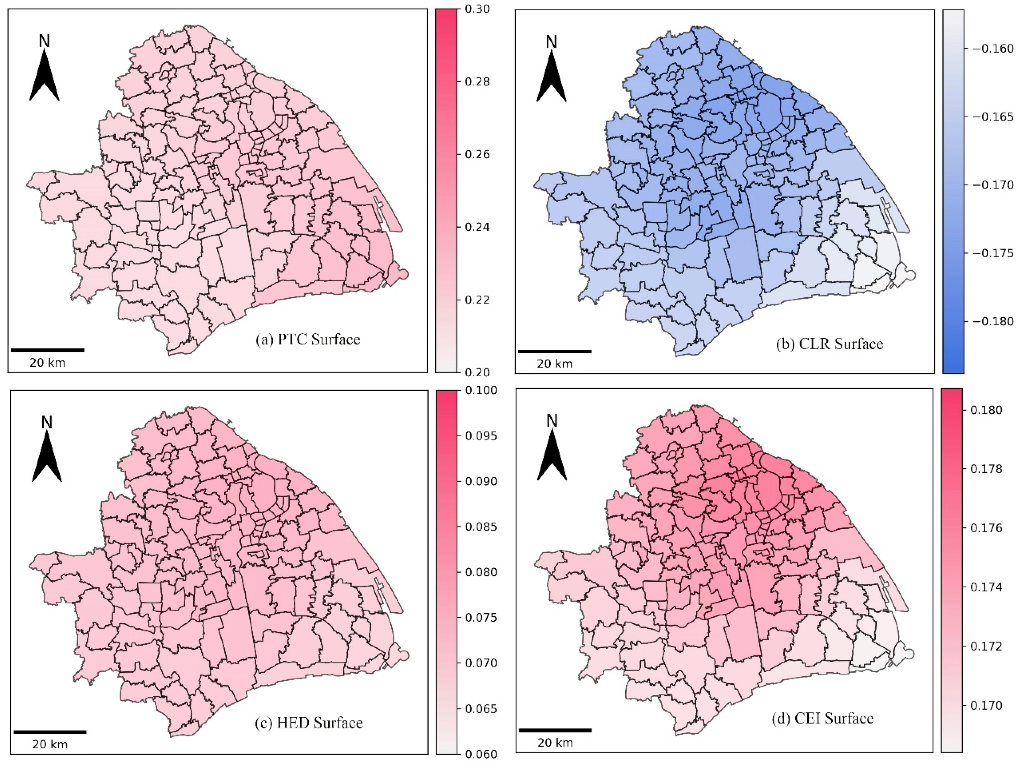
| Public transportation convenience (PTC) | 0.220 to 0.252 | 0.23 |
| Consumption level of residents (CLR) | −0.184 to −0.157 | −0.18 |
| High-tech enterprise density (HED) | 0.070 to 0.083 | 0.08 |
| City ecological index (CEI) | 0.168 to 0.180 | 0.17 |
| Model diagnosis | ||
| R-squared | 0.92 | |
| Number of effective parameters | 14.58 | |
| AIC | −194.57 | |
| Test | Value | p-value |
|---|---|---|
| Lagrange Multiplier (lag) | 39.53 | 0.00 |
| Robust LM (lag) | 0.20 | 0.66 |
| Lagrange Multiplier (error) | 85.67 | 0.00 |
| Robust LM (error) | 46.33 | 0.00 |
| Predictor Variable | SEM Parameter Estimation | MGWR Parameter Estimation | ||
|---|---|---|---|---|
| Coefficient | p-value | Range of Coefficient | Mean | |
| Intercept term (location in the MGWR) | −11.42 | 0.00 | −2.695 to 2.805 | −0.05 |
| Average floor area ratio (AFAE) | 0.78 | 0.00 | −0.449 to 1.426 | 0.52 |
| Public transportation convenience (PTC) | 0.11 | 0.01 | 0.220 to 0.252 | 0.23 |
| Consumption level of residents (CLR) | −0.25 | 0.00 | −0.184 to −0.157 | −0.18 |
| High-tech enterprise density (HED) | 0.02 | 0.24 | 0.070 to 0.083 | 0.08 |
| City Ecological index (CEI) | 0.07 | 0.00 | 0.168 to 0.180 | 0.17 |
| Lambda | 0.87 | 0.04 | ||
| Model diagnosis | SEM | MGWR | ||
| R-squared | 0.88 | 0.92 | ||
| Number of effective parameters | 6 | 14.58 | ||
| AIC | −126.93 | −194.57 | ||
Publisher’s Note: MDPI stays neutral with regard to jurisdictional claims in published maps and institutional affiliations. |
© 2021 by the authors. Licensee MDPI, Basel, Switzerland. This article is an open access article distributed under the terms and conditions of the Creative Commons Attribution (CC BY) license (https://creativecommons.org/licenses/by/4.0/).
Share and Cite
Cao, X.; Shi, Y.; Zhou, L.; Tao, T.; Yang, Q. Analysis of Factors Influencing the Urban Carrying Capacity of the Shanghai Metropolis Based on a Multiscale Geographically Weighted Regression (MGWR) Model. Land 2021, 10, 578. https://doi.org/10.3390/land10060578
Cao X, Shi Y, Zhou L, Tao T, Yang Q. Analysis of Factors Influencing the Urban Carrying Capacity of the Shanghai Metropolis Based on a Multiscale Geographically Weighted Regression (MGWR) Model. Land. 2021; 10(6):578. https://doi.org/10.3390/land10060578
Chicago/Turabian StyleCao, Xiangyang, Yishao Shi, Liangliang Zhou, Tianhui Tao, and Qianqian Yang. 2021. "Analysis of Factors Influencing the Urban Carrying Capacity of the Shanghai Metropolis Based on a Multiscale Geographically Weighted Regression (MGWR) Model" Land 10, no. 6: 578. https://doi.org/10.3390/land10060578