The Effects of Land Use on Concentrations of Nutrients and Selected Metals in Bottom Sediments and the Risk Assessment for Rivers of the Warta River Catchment, Poland

Abstract

Changes in the environment, aiming at agricultural intensification, progressive urbanisation and other forms of anthropopression, may cause an increase in soil erosion and a resulting increase in the pollution inflow to surface water. At the same time, this results in increased nutrient pollution of bottom sediments. In this study, the concentrations of total nitrogen (TN), total phosphorus (TP), total organic carbon (TOC), calcium (Ca), iron (Fe) and potassium (K) were analysed using bottom sediment samples collected at 39 sites located along the entire length of the Warta River and its tributaries. Agricultural use of land adjacent to rivers was found to significantly degrade sediment quality, while anthropogenic land use (as defined by Corine Land Cover classification—CLC), unlike previous studies, reduces the pollution loads in the bottom sediments. Forest use also contributes to the reduction of the pollution load in sediments. It was found that the significance of the relationship between pollutant concentrations and land use depends on the length of the river–land interface. According to the analyses, the level of correlation between the analysed constituents depends on the use of land adjacent to rivers. The impact of agricultural land use has the strongest effect in the 1 km zone and 5 km in the case of anthropogenic land use. The results showed that the variability of total phosphorus TP concentrations is strongly correlated with the variability of iron concentrations. SPI values indicate that the risk to sediment quality is low due to TOC and Fe concentrations. In contrast, the risk of sediment pollution by TN and TP shows greater differentiation. Although the risk is negligible for 40% of the samples, at the same time, for 33% of the samples, a very high risk of pollution with both TN and TP was found.

1. Introduction

River sediments are an important part of the cycling of materials in the aquatic ecosystem. The understanding of the pollution processes of river bottom sediments is of great importance because it can be an indicator of the ecological health of waters [1]. Sediments can accumulate pollutants and act as a buffer to absorb and release pollutants into the aquatic environment [2]. Loads of constituents such as carbon, nitrogen and phosphorus in bottom sediments and their interrelationships enable identification of the sources of organic matter and its transformations. The ratios of these constituents are affected by several environmental factors such as climate [3,4], terrestrial inflows, morphometry and use of adjacent areas [5] or the mineralogical composition of sediments [6]. Biochemical and biological transformations taking place in sediments and at the water–sediment interface [7,8], as well as the hydrodynamic processes of sediment transport in riverbeds [9], are also of great importance for concentrations and mutual proportions of constituents that can be found in bottom sediments.

The land-use pattern of the area located in the catchment is one of the more important factors affecting the concentrations of nutrients, as well as other pollutants, in river bottom sediments [10]. Intense agricultural production can be a significant source of nutrient inputs to surface waters, both as diffuse and point sources of pollution [11,12]. This impact varies over time and depends, among other things, on changes in agricultural production technology [13]. Szatten and Habel [14] showed that the decrease of intensive agricultural areas results in the reduction of sediments and nutrients loads flowing into the reservoir. Additionally, urbanised areas were indicated as a source of surface water pollution [15,16] and, consequently, also bottom sediment pollution. However, as indicated by Khatri and Tyagi [15], the anthropogenic factors affecting water pollution in rural areas differ from those in urban areas. The chemical composition of bottom sediments of the water bodies located in urban and industrial areas shows anthropogenic enrichment with organic matter, phosphorus, calcium and trace elements [17]. An increase in impermeable surfaces in these areas increases surface runoff and erosion processes, causing an increased inflow of sediments to rivers [18]. In turn, afforested areas enable a reduction in the inflow of pollutants to watercourses and, consequently, reduce their deposition in bottom sediments. Riparian forest buffer systems are an effective tool for controlling the number of sediments and related pollutants carried in surface runoff [19]. Forest ecosystems also reduce the leaching of soluble nutrients into stream water [20]. In this regard, there is a frequent emphasis on the role of riparian vegetation that can act as a buffer to intercept suspended sediments and pollutants [21]. Forested riparian zones can reduce loads of suspended sediment in the runoff by 90% [22]. Grass riparian filter strips show a similar reduction of sediments in runoff as observed in forested zones, while the reduction of nitrogen and phosphorus is near 50% [23,24]. However, using only the primary type of land use may not be sufficient to explain the influx of pollutants to the aquatic environment fully. Liu et al. [6] showed that more fragmented forms of land use would give higher pollutant loads even if they are of the same primary type of land use.

The assessment of a qualitative status of bottom sediments requires the adoption of certain standards defining the concentrations of chemicals, the exceeding of which causes the sediments to be considered polluted. This is mainly due to the simplicity and ease of their application in practice. These standards, depending on a local controller, may address a variety of substances, including organic carbon, nutrients, heavy metals, organic compounds and others, and have different thresholds [25,26].

The chemicals that make up bottom sediments are interrelated. According to previous studies, the relationships between TN, TP and TOC concentrations are the result of biochemical and geochemical processes occurring in the environment and enable the identification of the sources of pollution [27,28]. Carbon–nitrogen ratio is one of the main variables to determine the source of organic matter in rivers [29]. Yun and An [30] indicated that the N:P ratio could be used in diagnosing the ecological health of a stream. Additionally, the relationships between TP concentrations and Fe, Ca and TOC concentrations are indicated, but the links between these elements can be different for each river [31].

The researches on the quality of riverine bottom sediments in lowland areas of Poland conducted in recent years has focused mainly on the analysis of concentrations and hazards caused by heavy metals [32,33,34], while the risks of nutrients or organic matter have not been analysed in detail.

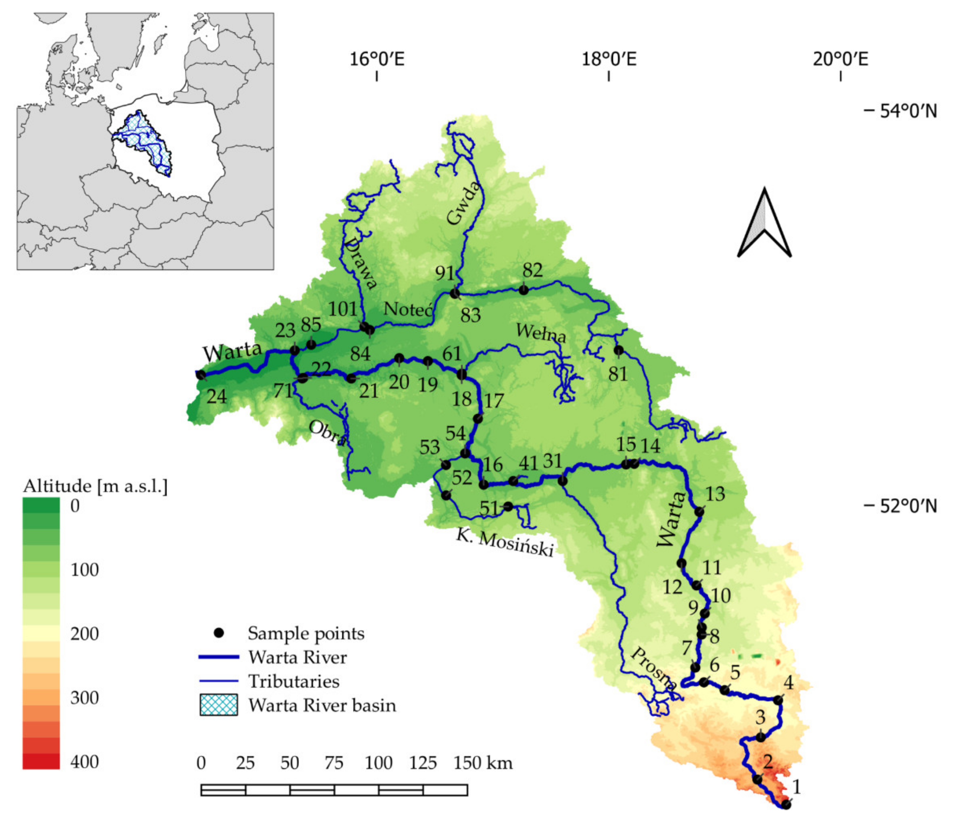
This study aims to analyse the spatial variability of TN, TP, TOC, Ca, Fe and K concentrations and their interrelationships in bottom sediments of the Warta River and its tributaries. The analysis also considered the effects of land cover structure and P, Ca and Fe concentrations in soils, found in areas adjacent to sediment sampling sites, on sediment composition for different lengths of the contact zone between the river and surrounding areas. This enables the assessment of sediment quality and the identification of factors affecting the concentrations of nutrients in sediments.

2. Materials and Methods

2.1. Site Description

The catchment area of the Warta River is 54,519 km². In terms of length, 808 km, it is the third-longest river in Poland (Figure 1). The tributaries of the Warta River, which were also analysed in the presented study, are the Prosna River; the Bobrowski Canal; the Mosiński Canal; the Wełna, Obra and Noteć rivers as well as the additional tributaries of the Noteć River: the Gwda and Drawa rivers (Figure 1). The source of the Warta River is 380 m above sea level, and its mouth to the Oder is 12 m above sea level. The catchment area of the Warta River varies in terrain. The upper-southern part of the catchment is located in the Kraków-Częstochowa Upland, passing through the Central Polish lowlands to the northern lake districts. The tributaries of the Warta River range from 11 km (the Bobrowski Canal) to 391 km (the Noteć River). Their areas range from 28 km² in the case of the Bobrowski Canal to 17,319 km² in the case of the Noteć River (

Table 1. Analysed rivers’ descriptions.

River	Length (km)	Basin Area (km2)	Corine Land Cover (%)
			1	2	3	4	5
Warta	808	54,519	5.6	60.2	32.5	0.2	1.4
Prosna *	227	4920	5.9	72.0	21.8	0.1	0.2
Kanał Bobrowski *	11	28	4.3	61.0	34.6	0	0
Kanał Mosiński *	142	2503	5.0	77.8	15.9	0.3	1.1
Wełna *	118	2620	3.6	72.0	22.5	0.1	1.8
Obra *	183	2759	3.8	50.7	43.7	0.2	1.6
Noteć *	391	17,319	3.1	51.0	43.1	0.3	2.4
Gwda **	145	4963	3.4	40.7	53.1	0.2	2.6
Drawa **	192	3290	2.0	32.2	61.8	0.1	3.9

Crine Land Cover: 1—Artificial surfaces, 2—Agricultural areas, 3—Forest and semi-natural areas, 4—Wetlands, 5—Water bodies; *—primary Warta tributary, **—secondary Warta tributary (via Noteć).

).

Almost along the entire length of the Warta river as well as its tributaries drains a post-glacial landscape formed during the retreat of the Vistulian ice-sheet. The layer of glacial sediments with a thickness of more than 200 m consists of tills, glacial sands and gravels and outwash sands and gravels [35]. In the Warta River catchment area, sandy soils make up 45% of the land area, clay soils 41% and organic soils and alluvial soils 14% of the land area [36]. According to the European Soil Database v2.0 m, the main soils are Podzol—32%, Luvisols—30%, Fluvisols—12% and Arenosols—12%.

According to the CLC classification, in the whole catchment area of the Warta River, agricultural land use makes up 60.2% of the catchment area, forest and semi-natural land use make up 32.5%, anthropogenic land use makes up 5.6%, surface water makes up 1.4% and the rest is covered by wetlands and peat moors (Table 1, Figure 2).

The highest proportion of agricultural land has the catchment area of the Mosiński Canal—approximately 78%. This catchment also has the lowest proportion of forest land and semi-natural land in a total catchment area—less than 16%. A slightly lower, compared to the aforementioned catchment, proportion of agricultural land in the total catchment area, 72%, is found in the catchment areas of the Prosna and Wełna rivers. On the other hand, the catchment area with the highest proportion of forest land and semi-natural forest land is the Drawa River catchment located in the northern part of the Warta catchment, where this proportion is 61.8%. This catchment also has the highest proportion of the open water area—3.9% of the total catchment area. The proportion of wetlands in all catchments is very small, reaching a maximum of 0.3% for the Mosiński Canal catchment.

An important source of bottom sediment contamination is the material brought into rivers as a result of erosion processes. One of the indicators that identify areas sensitive to erosion is the Topographic Wetness Index TWI. The TWI takes into account the upslope area and its slope, allowing the calculation of the steady-state wetness and runoff across the analysed area. Calculated TWIs show values in the range of 0.9–14.4 and are shown in Figure 3.

Geochemical conditions in the Warta River catchment, which describe the phosphorus, calcium and iron concentrations found in a 20 cm topsoil, are shown in Figure 4.

The Warta River catchment has the lowest annual precipitation in Poland [37]. Climatologically, according to the Köppen–Geiger’s classification, the catchment area is located in the oceanic climate (Cfb) that has warm summers and milder winters [38,39]. The average annual air temperature for the WRC is approximately 8 °C, while the annual precipitation ranges from 520 mm in the north-eastern part of the catchment to 675 mm in the southern part [40]. The mean annual runoff is 3.86 dm³·s⁻¹·km⁻² for the Warta catchment and it shows considerable spatial variability [41]. The lowest runoff values, below 2 dm³·s⁻¹·km⁻², are observed in the upper catchment of the Noteć River [42].

2.2. Materials

The analyses used data concerning the measurements of N, P, K, Ca, Fe and TOC concentrations in bottom sediments of the Warta River and its tributaries, which were obtained as part of the State Monitoring of the Natural Environment programme. Bottom sediment samples were collected from 39 sites in 2016 (Figure 1). Sampling sites were located at the borders of the catchment area, at the mouths of tributaries and below cities where large industrial plants are located. For chemical analyses, a 5 cm top layer of sediments was collected from 4–5 sites over a 50 m distance for each location using a van Veen grab sampler. Samples for each site were mixed and rubbed through a nylon sieve with 2 mm mesh. Laboratory measurements were performed for Ca, K, Fe and P using inductively coupled plasma atomic emission spectrometry (ICP-AES) according to PN-EN 13657:2006, PN-EN ISO 11885:2009. Total organic carbon (TOC) was measured using coulometric titration according to CZ_SOP_D06_07_055 (CSN ISO 10694, CSN EN 13137). Kjeldahl nitrogen was determined using titration according to PN-EN 13342:2002.

The boundaries of the catchment area of the Warta River, its course and the course of its analysed tributaries were determined based on a Computer Map of the Hydrographic Division of Poland, which contains full hydrographic data of Poland in vector format. The land-use structure in the catchment area was made based on the CLC database provided by the Chief Inspectorate for Environmental Protection. The landform was described using a Digital Elevation Model (DEM) on a grid of at least 100 m, which was obtained from the Central Office of Geodesy and Cartography. The Ca, Fe and P concentrations found in the 20 cm topsoil were estimated using the Geochemical Atlas of Poland at a scale of 1:500,000, which was obtained from PGI—PIB (Polish Geological Institute—National Research Institute).

2.3. Methods

2.3.1. Overall Statistics

To evaluate the variability of N, P, K, Ca, Fe and TOC concentrations in bottom sediments of the analysed rivers, the mean values of the concentrations, the median and their maximum and minimum values were calculated. Concentration distributions were determined using the Shapiro–Wilk test. Outliers were determined using the Interquartile Range (IQR) test. The values that fall below or above 1.5-IQR were considered as outliers of the variables:

Up = Q₃ + 1.5·IQR

(1)

Low = Q₁ − 1.5·IQR

(2)

where Up—concentrations for values that fall above the 75th quartile (${\mathrm{Q}}_3$) and Low—concentrations for values that fall below the 25th quartile (${\mathrm{Q}}_1$). Correlations were determined using Spearman’s rank coefficients.

All statistical calculations and visualisation of results were performed using R version 4.0.5.

2.3.2. Risk Assessment Method

An ecological risk assessment of nutrients in river bottom sediments was performed using a method based on the Single Pollution Index (SPI) [43].

The SPI_i is calculated based on the formula:

SPI_i = C_i/C_s

(3)

where C_i is a measured concentration of the evaluated i factor and C_s is a standard concentration of the evaluated i factor. Calculations were performed for TN, TP, TOC and Fe. Values of 550 mg-kg⁻¹, 600 mg-kg⁻¹, 1% and 2% were used as standard values for TN, TP, TOC and Fe, respectively, which are derived from safe nutrient concentration limits that can be found in the Sediment Quality Guidelines [25,43]. Based on the P_i, four hazard classes can be distinguished as shown in

Table 2. Single pollution index SPI_i classification.

Risk Level	TN	TP	TOC	Fe	Sediment Pollution
I	PTN < 1	PTP < 0.5	PTOC < 1	PFe < 0.5	Clean
II	1 ≤ PTN < 2	0.5 ≤ PTP < 1	1 ≤ PTOC < 5	0.5 ≤ PFe < 1	Slightly polluted
III	2 ≤ PTN < 3	1 ≤ PTP < 1.5	5 ≤ PTOC < 10	1 ≤ PFe < 2	Moderately polluted
IV	3 ≤ PTN	1.5 ≤ PTP	10 ≤ PTOC	2 ≤ PFe	Seriously polluted

[43].

C:P:N stoichiometry enables the description of potential sources of pollution as well as geochemical and biochemical processes occurring in the environment [31,44]. TOC/TN is one of more frequently used ratios, which identifies potential sources of organic matter [43]. TOC/TP reflects to some extent the rate of conversion of organic carbon and phosphorus compounds [45]. In contrast, TN/TP reflects the dynamics of accumulation, deposition and release of nitrogen and phosphorus in water [46,47]. TOC/TN > 10 indicates primarily a terrestrial source of organic matter. In contrast, TOC/TN < 10 indicates an aquatic source of organic matter. TOC/TN~10 indicates that the organic matter found in sediments is of both terrestrial and aquatic origin [48,49].

2.3.3. Analyses of Spatial Variability of Concentrations of Selected Elements Found in Bottom Sediments

The principal component analysis (PCA) and cluster analysis (CA) were used for the differentiation of groups of sampling sites exhibiting similar variability and similar sources. Due to concentrations of analysed substances in bottom sediments, the cluster analysis of sampling sites was performed using k-medoids [50,51]. K-medoids is a technique that is less sensitive to the effect of noise and outliers in analysed data, compared to the k-means. The number of cluster groups was found using the silhouette method [52].

Land cover was defined for river-adjacent zones of a width of 500 m, in % of the total area of the zone. The adopted zone lengths were 1, 2, 5 and 10 km from the sampling sites (Figure 5). In zones defined as above, GBI’s content index for P, Ca and Fe was also calculated based on the formula:

GBI = Σ(GBC_i·A_i)/ΣA_i

(4)

where GBC_i means the topsoil content class for each element, while A_i is the area per class in an analysed zone.

Spatial variability data concerning the parameters were determined using QGIS 3.18 whereas statistical calculations were performed using R 4.0.

3. Results and Discussion

3.1. General Characteristics of Concentration Variability

The results of measurements made in 2016 for TN, TP, Ca, Fe and TOC concentrations found in the bottom sediments of the Warta River and its tributaries are shown in

Table A1. Concentrations of chosen elements (mg·kg⁻¹) and TOC (% d.m.) in the bottom sediments of the Warta river.

River	Site No.	TN	TP	TOC	Ca	Fe	K
Warta	1	207	276	0.568	22,430	9460	170
	2	491	217	1.98	630	3200	129
	3	331	320	2.27	2232	6640	216
	4	16,240 *	3405 *	21.5 *	21,810	38,180	1384
	5	260	193	1.24	3398	4270	212
	6	354	220	0.643	1705	3608	100
	7	71.5	48.8	0.202	423	2518	332
	8	156	108	0.233	2010	3044	137
	9	82.7	294	0.375	3068	4877	237
	10	330	283	1.84	1457	4840	255
	11	211	464	2.36	2050	6874	227
	12	1380	881	5.15	8420	20,300	1192
	13	127	71.9	0.26	760	2017	117
	14	701	927	1.93	4081	12,760	511
	15	3040	1419	3.49	8486	15,870	950
	16	219	186	0.709	808	2626	116
	17	1380	1756	2.18	11,470	17,550	1428
	18	998	683	2.53	3467	8269	440
	19	1100	3280 *	4.99	8288	21,160	879
	20	3070	3054 *	3.86	11,990	19,380	1119
	21	935	573	6.22	3285	6640	325
	22	367	251	1.43	3763	8368	470
	23	4630	3773 *	5.51	15,090	39,680 *	2731 *
	24	650	108	2.38	999	1602	122
Prosna	31	1560	837	1.66	3188	13,800	726
K. B. 1	41	3490	631	7.34	5985	14,310	320
Kanał Mosiński	51	1860	1229	0.839	54,010 *	22,070	2994 *
	52	188	427	1.52	2637	7734	276
	53	3950	1638	2.71	41,250 *	20,050	1197
	54	1560	1213	1.6	11,590	14,000	890
Wełna	61	169	126	0.818	1915	1964	211
Obra	71	2920	1145	3.42	12,160	18,610	1169
Noteć	81	544	228	1.25	13,630	8174	1828
	82	11,040 *	8864 *	18.2 *	21,200	68,280 *	1208
	83	4230	275.3	13.8 *	8257	7041	556.1
	84	4790	2000	9.37 *	12,990	18,750	874.6
	85	1970	332	1.74	6388	4937	416.8
Gwda	91	7550 *	1992	5.78	18,050	23,800	1584
Drawa	101	1450	324.2	2.55	8108	6835	505.7

¹ Kanał Bobrowski, * outliers.

. Concentrations of individual elements are within N: 71.5–16,240 mg-kg⁻³, P: 48.8–8864 mg-kg⁻¹, Ca: 423–54,010 mg-kg⁻¹, Fe: 1602–68,280 mg-kg⁻¹ and TOC: 0.20–21.50 % d.m.

The average concentrations of the analysed elements ranged from 13,182 mg-kg⁻¹ for Fe through 9320 mg-kg⁻¹ for Ca, 2169 mg-kg⁻¹ for N to 1130 mg-kg⁻¹ for P and 3.76% for TOC (

Table 3. The descriptive statistics concentrations of chosen elements (mg·kg⁻¹) and TOC (% d.m.).

Site No.	TN	TP	TOC	Ca	Fe
min	71.5	48.8	0.20	423	1602
median	998	464	2.18	5985	8269
mean	2169	1130	3.76	9320	13,182
max	16,240	8864	21.50	54,010	68,280
range	16,169	8815.2	21.298	53,587	66,678
sd	3244	1619	4.70	11,078	12,930
skew	2.68	3.00	2.33	2.29	2.27
kurtosis	7.79	10.81	5.16	5.80	6.42
IQR	2685	1084.5	3.18	9934	13,821.5

). The median values are 8269 mg-kg⁻¹, 11,078 mg-kg⁻¹, 998 mg-kg⁻¹, 464 mg-kg⁻¹ and 2.18% for Fe, Ca, N, P and TOC, respectively. The TOC values measured in 1998–2000 are similar to those measured in bottom sediments of the Oder, which is a receiving body for the water of the Warta River, when they ranged from 0.2% d.m. to 18.2% d.m., averaging 4.9% d.m [53]. Similar values for P, Ca, Fe and TOC concentrations were observed by House and Denison [31,54] in seven rivers in southern England. Their reported data concerning concentrations were 40–47,000 mg-kg⁻¹ for Fe, 40–19,000 mg-kg⁻¹ for Ca, 10–2000 mg-kg⁻¹ for P and 0.6–19% d.m. for TOC. This may indicate similar sources of sediment pollution and similar land use of catchments.

The IQR values shown in Table 3 were 2685 mg-kg⁻¹, 1084 mg-kg⁻¹, 9934 mg-kg⁻¹, 13,821 mg-kg⁻¹ and 3.18% for TN, TP, Ca, Fe and TOC, respectively. The IQR test showed several outliers involving N concentrations in the Warta River bottom sediments at site no. 4 and the Noteć River sediments at site no. 82. For phosphorus, concentration outliers were found in the Warta River sediments at sites no. 4, 19, 20 and in the Noteć River sediments, at site no. 82. For Ca, outliers were observed in the Mosiński Canal at sites no. 51 and 53. For Fe, outliers were found in the Noteć River at site no. 82. Outlier TOC values were observed in the Warta River sediments at site no. 4 and in the Noteć River bottom sediments at sites no. 82, 83 and 84. The outliers were most frequently observed at site no. 82 (Noteć River)—four times and three times higher/lower at sites no. 4 and 23 (Warta River).

The analysis of distributions of the analysed concentrations showed that none of the concentration distributions is a normal distribution (Figure 6). In contrast, for all p > 0.05 parameters, all distributions are similar to a log-normal distribution.

All analysed concentrations are strongly positively correlated with one another. Spearman’s correlation coefficients range from 0.50 for the correlation between TOC and Ca to 0.93 for the correlation between TP and Fe. Almost all correlation coefficients are significant at the p < 0.0001 level (

Table 4. Correlation coefficients between analysed elements.

	TN	TP	TOC	Ca	Fe
TP	0.79	-
TOC	0.82	0.71	-
Ca	0.74	0.76	0.50	-
Fe	0.79	0.93	0.65	0.87	-
K	0.74	0.79	0.54	0.83	0.86

). Only the TOC–Ca correlation is significant at the p < 0.01 level, whereas the TOC–K correlation is significant at the p < 0.001 level. The strongest correlation is between Fe concentrations and TP, Ca and K concentrations, for which the correlation coefficients are 0.93, 0.87 and 0.86, respectively. In contrast, the correlations between TOC and Ca/K are the least correlated, but still significant at the p < 0.01 level.

Inorganic constituents that can combine with or adsorb phosphates are one of the factors affecting TP concentrations in bottom sediments [55,56]. Immobilising components include metals, such as iron, which combine with phosphorus, forming crystalline metal phosphates (e.g., strengite or vivianite), or they can adsorb phosphorus on the oxide/hydroxide layer. In the case of the presence of large amounts of calcium, phosphate precipitation may occur in the form of hydroxylapatite (HA) or various calcium phosphates [55,57,58]. Furthermore, iron (III) plays an important role in the phosphate sorption by humic elements, forming iron (III)–humus complexes with phosphates [55,59].

3.2. C:N:P Stoichiometry

The calculated characteristic values of C:N, C:P and N:P ratios indicate their high variability as shown in

Table 5. Descriptive statistics of C:N, C:P and N:P ratios.

Item	Min	Median	Mean	Max	1st Qu	3rd Qu	SD
C:N	4.51	22.98	30.1	111.85	12.90	39.65	22.91
C:P	6.83	37.04	58.3	501.27	20.55	63.70	82.68
N:P	0.28	1.47	2.32	15.37	1.18	2.40	2.61

and Figure 7. C:N values range from 4.51 to nearly 112, with a median value of 22.98. The highest C:N values of 112, 81, 68 and 61 were observed at sites no. 11, 52, 3 and 21, respectively. A total of 33 sites had C:N > 10, two sites had ratios similar to 10, and only four sites had C:N < 10 (Figure 7). This indicates that the organic matter found in bottom sediments derives mainly from runoff from surrounding areas. Similarly, high C:N values were also obtained by Lu [60], indicating that exogenous sources of pollution are the cause. On the other hand, the lowest C:N values have sediments at sites located in the vicinity of the aforementioned site no. 52, i.e., sites no. 51 and 53–4.5 mg-kg⁻¹ and 6.9 mg-kg⁻¹, respectively. The bottom sediments at these two sites have high nitrogen concentrations as well as very high P, Ca and Fe concentrations (Table A1).

C:P ratio values in bottom sediments of rivers of the Warta River catchment ranged from 6.83 to 501.27, with a mean value of 58.3. The highest value of this parameter was obtained for site no. 83—the Noteć River, while the lowest for site no.—the Mosiński Canal.

N:P ratios in the bottom sediments of rivers of the Warta River catchment ranged from 0.28 to 15.37, with a mean value of 2.32. According to Chen et al. [45], low N:P values correspond to eutrophic and mesotrophic conditions with the predominant supply of nutrients derived from external sources. The nutrients from such sources are complex and have low N:P ratios. In contrast, high TN/TP values can be observed under oligotrophic conditions when natural nutrient supply sources have high N:P ratios. Knösche [55] reports that the TN:TP ratio in river sediments decreases significantly from low-density Paleopotamal sediments (median TN:TP = 23.7) to high-density Eupotamal sediments (median 8.5). He also observed a similar correlation for the TOC:TP ratio. At the same time, Ostendorp [61] indicated that N:P:OC ratios could be explained by the variability of organic content rather than by eutrophication processes in each case.

3.3. Single Pollution Index (SPI)

The pollution status of bottom sediments of the rivers of the Warta River catchment shows great spatial variation, as shown in Figure 8. SPI values for nitrogen range from 0.13 to 29.5. The largest proportion of sediment samples, 41%, can be classified as Class I (

Table 6. SPI classes distribution for Warta River basin in %.

Site No.	I	II	III	IV
TN	41	13	13	33
TP	39	15	10	36
TOC	23	54	15	8
Fe	56	23	18	3

). Class II includes 13% of the samples. Sampling sites with a low risk of nitrogen pollution are located mainly in the upper part of the Warta River (sites no. 1–14, excluding sites no. 4 and 12) and in its lower reaches (sites no. 18–24, excluding site no. 20). On the other hand, Class III includes 13% of sediment samples and Class IV, with the highest pollution, includes as many as 33% of samples. These sites are located primarily in the middle course of the Warta River and in its tributaries.

SPI values for sediments polluted with phosphorus ranged from 0.08 to 14.8. Classification of sediment samples classifies 39% of samples into Class I, 15% into Class II, 10% into Class III and 36% into Class IV. These values are similar to SPI for TN. As with nitrogen, the sampling sites classified as Class I and II are located in the upper and lower reaches of the Warta River. The SPI values for TOC allow 23% of sediment samples to be classified as Class I and 54% as Class II. On the other hand, 15% and 8% of sediment samples should be classified into Class III and IV, respectively. This indicates a much lower risk of bottom sediment pollution by TOC than by TN or TP. The lowest pollution risk to bottom sediments was found for Fe. SPI values ranging from 0.08 to 3.4 enabled 56%, 23%, 18% and 3% of the samples to be classified as classes II–V, respectively.

The obtained SPI values indicate a lower pollution risk to bottom sediments of the Warta River than those obtained by He et al. [43] for Chinese rivers.

3.4. Spatial Variation of Pollutant Concentrations

The clustering analysis of TN, TP, TOC, Ca, Fe and K concentrations in bottom sediments using the Partitioning Around Medoids (PAM) identified three groups of bottom sediment sampling sites (Figure 9). A simultaneous principal component analysis (PCA) found that the first two principal components, for which the eigenvalues are greater than 1, explain approximately 87% of the total variance (

Table 7. Eigenvalues, percent of variance and cumulative percent of variance for the PCA.

Component.	Eigenvalue	Percent of Variance	Cumulative Percent of Variance
1	4.0463	67.44	67.44
2	1.1709	19.52	86.96
3	0.4460	7.43	94.39
4	0.2323	3.87	98.26
5	0.0799	1.33	99.59
6	0.0247	0.41	100.00

).

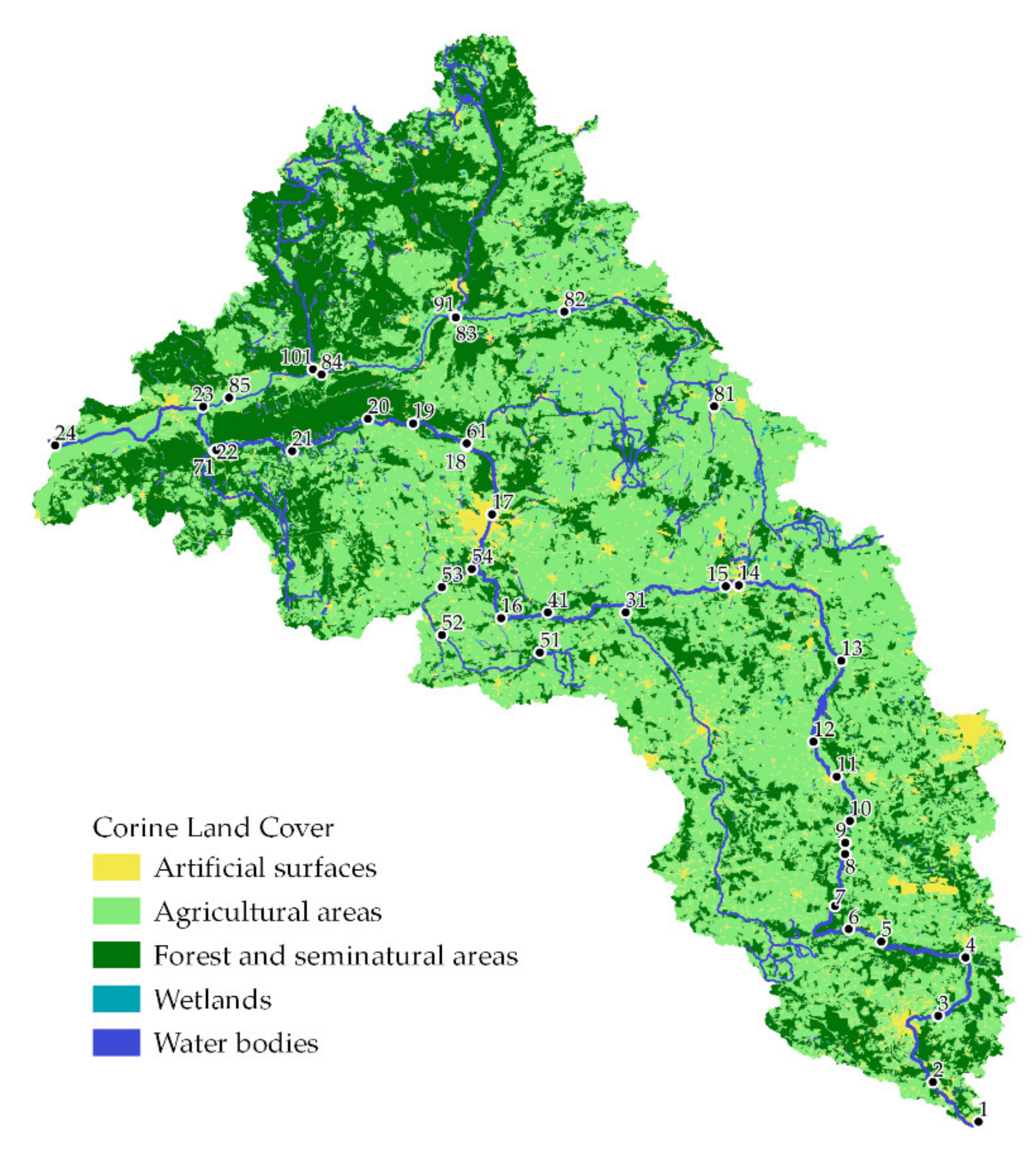
The land-use structure, as determined by the CLC classification, shows varying effects on the levels of constituents found in river sediments of the Warta River catchment. Anthropogenic lands (C_1) and forests and semi-natural ecosystems (C_3) show a negative correlation, while agricultural lands (C_2) and lands covered by water (C_5) show a positive correlation with concentrations of all elements; however, this relationship is not statistically significant in most cases. It should be noted that previous studies highlighted the negative impact of urbanised areas on the quality of bottom sediments in rivers. This was mainly due to the impact of direct discharge of wastewater into rivers or increasing surface runoff from areas with impervious surfaces [62,63]. However, the following phenomena that have been marked in recent years, such as the connection of most wastewater sources to wastewater treatment plants, the increase of areas that enable rainwater infiltration or, for example, measures to retain rainwater runoff from impervious surfaces, may reduce or neutralise the negative impact of urbanisation on the quality of surface water and bottom sediments. The negative impact of agricultural areas is mainly caused by an increased input of nutrients [12], inorganic suspended solids [64] and organic matter [65] from these areas to surface waters.

Factor loadings for the first two principal components are shown in

Table 8. Loading for PCA matrix.

	Components
	1	2
TN	0.888 **	−0.295
TP	0.887 **	−0.172
TOC	0.798 **	−0.500 *
Ca	0.651 *	0.649 *
Fe	0.957 **	−0.045
K	0.704 *	0.617 *

**—strong effect; *—moderate effect.

. According to the classification presented by Liu et al. [66], factor loadings were classified as “strong,” “average,” and “weak” for values of >0.75, 0.75–0.50, and 0.50–0.30, respectively. PC1, which explains 67.4% of the total variance, has strong positive Fe, TN, TP and TOC loadings, while also showing average K and Ca loadings.

Table 9. Correlation coefficient matrix showing element–land cover and element–geochemical background relationships in sediments.

Buffer Length (km)	Parameter	N	P	TOC	Ca	Fe	K
1	C_1	−0.23	−0.28	−0.34 *	−0.28	−0.24	−0.30
	C_2	0.36 *	0.33 *	0.40 *	0.37 *	0.39 *	0.41 **
	C_3	−0.29	−0.14	−0.17	−0.31	−0.30	−0.31
	C_4	-	-	-	-	-	-
	C_5	0.09	0.35 *	0.19	0.24	0.13	0.19
2	C_1	−0.22	−0.26	−0.35 *	−0.27	−0.24	−0.31
	C_2	0.29	0.28	0.36 *	0.29	0.29	0.35 *
	C_3	−0.24	−0.11	−0.15	−0.22	−0.24	−0.27
	C_4	-	-	-	-	-	-
	C_5	0.12	0.34 *	0.21	0.27	0.17	0.24
5	C_1	−0.27	−0.32 *	−0.37 *	−0.26	−0.34 *	−0.32 *
	C_2	0.10	0.10	0.14	0.07	0.14	0.13
	C_3	−0.18	−0.03	−0.09	−0.13	−0.18	−0.18
	C_4	-	-	-	-	-	-
	C_5	0.20	0.42 **	0.32 *	0.34 *	0.25	0.32 *
10	C_1	0.00	−0.31	−0.19	−0.12	−0.07	−0.12
	C_2	0.14	0.22	0.21	0.17	0.24	0.19
	C_3	−0.30	−0.15	−0.20	−0.22	−0.33 *	−0.28
	C_4	0.04	0.25	0.20	−0.12	0.04	−0.04
	C_5	0.10	0.34 *	0.21	0.21	0.14	0.17
2	Ca_geo	0.17	0.22	0.18	0.17	0.05	0.15
	Fe_geo	0.24	0.16	0.24	0.08	0.19	0.07
	P_geo	0.36 *	0.35 *	0.45 **	0.32 *	0.41 **	0.29

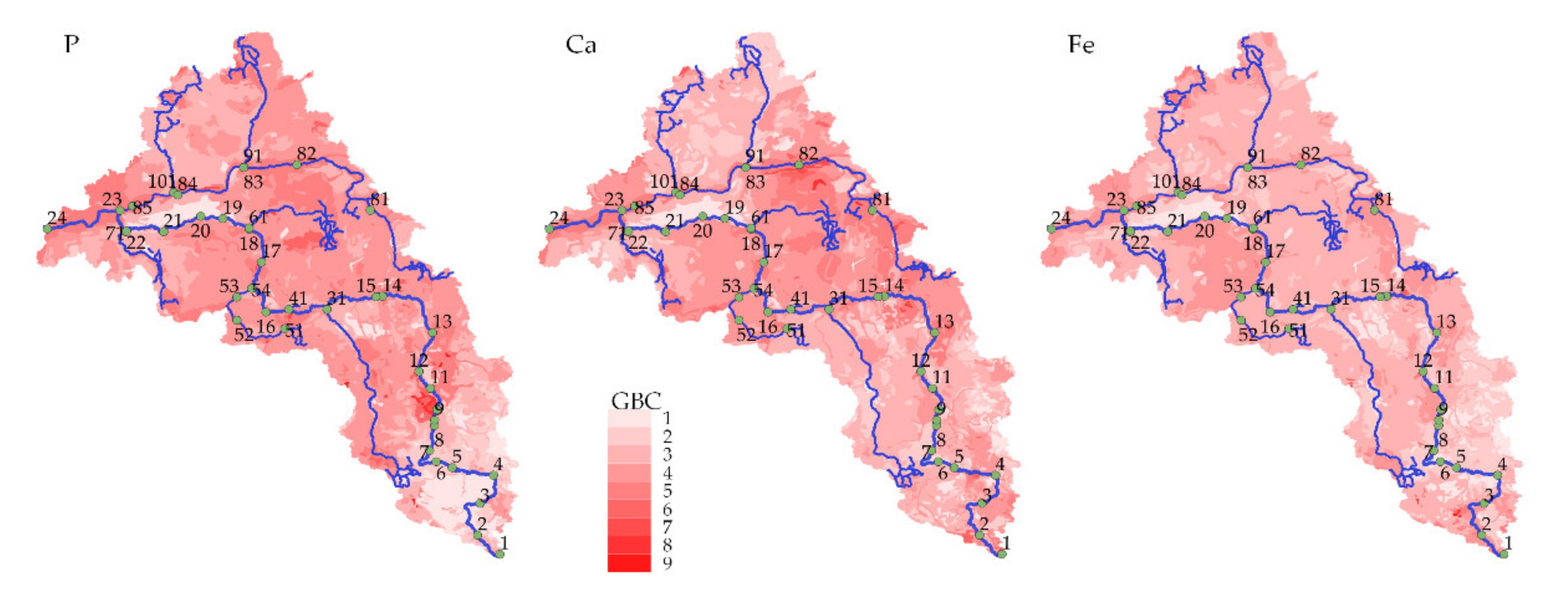
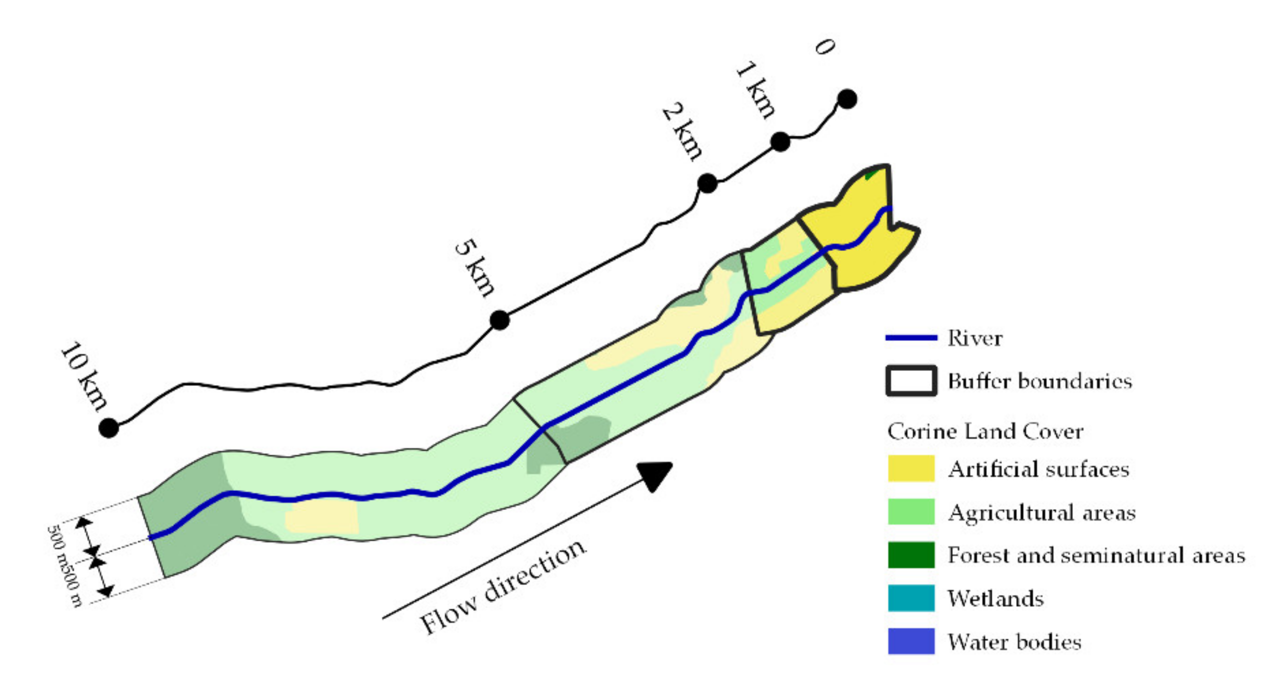
*—significant at p < 0.05; **—significant at p < 0.01; Land Cover: C1—Artificial, C2—Agricultural, C3—Forests and seminatural, C4—Wetlands, C5—Water.

shows the Spearman’s correlation coefficient values of TN/TP/K/Ca/Fe/TOC concentrations in bottom sediments with land cover structure in the zones of a width of 1000 m, adjacent to the river on a length of 1, 2, 5 and 10 km, and the calculated Ca, Fe and P content index of the topsoil.

The significance of the land-use impact depends not only on the land-cover structure itself, but also on the length of the contact zone of land adjacent to the watercourse. A significant (p < 0.05) effect of agricultural land (C_2) on the concentration levels of all analysed elements was observed for the 1 km buffer area. For longer buffer lengths, excluding K and TOC concentrations in the 2 km buffer area, that effect was no longer statistically significant. In contrast, the proportion of anthropogenic land (C_1) is significantly linked to P, K, Fe and TOC concentrations in the 5 km buffer area. Additionally, the proportion of the area covered by water (C_5) shows the strongest relationships with P, K, Ca and TOC concentrations in the 5 km buffer area. At the same time, the proportion of the land covered by water is the only one that is significantly correlated with phosphorus concentrations for all buffer lengths. Except for the effects of forest land proportion (C_3) on Fe concentrations in the 10 km buffer area, there was no significant impact of that land-use category on concentrations of analysed substances found in bottom sediments.

The results indicate a significant positive relationship between the geochemical background level of phosphorus in the 2 km buffer area and N, P, Ca, Fe and TOC concentrations in the bottom sediments analysed. In contrast, the geochemical background levels of Ca and Fe do not show such a relationship.

3.5. The Relationships between Water Quality Parameters and Land Use

The analysis of land use as identified based on the CLC data in individual buffers enabled four land-cover groups to be distinguished. The clustering results and the distribution of each group are shown in Figure 10. The first group includes areas dominated by anthropogenic lands, with a low proportion of forests. The second group includes buffer areas that are predominantly forested. The third group includes buffer areas dominated by agricultural lands. The fourth group consists of buffer areas where the proportion of lands covered by water is at least 10%, regardless of other land-use categories.

The Spearman’s correlation coefficients between parameters describing constituent concentrations in bottom sediments for defined land-use groups are shown in

Table A2. The correlation coefficients between the concentrations of elements in the bottom sediments for buffer zones with various land covers.

	TN	TP	TOC	Ca	Fe
Anthropogenic land cover (cluster 1, n = 8)
TP	0.86 **
TOC	0.69	0.76 *
Ca	0.36	0.40	0.05
Fe	0.83 *	0.93 ***	0.52	0.62
K	0.76*	0.62	0.52	0.60	0.69
Forest land cover (cluster 2, n = 8)
TP	0.95 ***
TOC	0.93 ***	0.83 *
Ca	0.79 *	0.79 *	0.86 **
Fe	0.86 **	0.90 **	0.81 *	0.83 *
K	0.57	0.52	0.69	0.74 *	0.69
Agricultural land cover (cluster 3, n = 17)
TP	0.74 ***
TOC	0.86 ***	0.60 *
Ca	0.76 ***	0.80 ***	0.50 *
Fe	0.75 ***	0.92 ***	0.62 **	0.88 ***
K	0.74 ***	0.81 ***	0.49 *	0.93 ***	0.92 ***
Water land cover (cluster 4, n = 6)
TP	0.89 *
TOC	0.60	0.60
Ca	0.83 *	0.89 *	0.26
Fe	0.77	0.94 **	0.31	0.94 **
K	0.83 *	0.89 *	0.26	1.00 ***	0.94 **

*—p < 0.05, **—p < 0.01, ***—p < 0.001; n—number of samples.

. In group 1, where anthropogenic land use is the main factor, the strongest relationship is between TP and Fe, TN and TOC concentrations. However, the relationships between the elements show a higher correlation in the case of buffers that were identified based on a significant proportion of forest land. The highest correlation is between TP and TN, TN and TOC and TP and Fe. Unlike cluster 1, there is also a strong correlation between TOC and Fe in cluster 2.

The highest levels of correlation between bottom sediment constituents occur when the river is adjacent to agricultural land (cluster 3). In this case, all correlation coefficients are statistically significant, at least at the p < 0.05 level. The highest correlation in cluster 3 is between Ca and K, TP and Fe and Fe and K. The lands included in cluster 4 have surface water within the buffer area, the proportion of which is between 10% and 20% (highest proportion) of the total buffer area. In the case of sediment samples collected at sites assigned to this cluster, the highest correlation occurred between Ca and K concentrations, where r = 1.0. Again, very high levels of correlation occurred between Fe and TP and Ca and K.

It should be noted that regardless of the influence of the environment, phosphorus concentrations show the highest correlation with iron concentrations and slightly lower correlation with calcium concentrations, which is due to the already mentioned mutual interactions between these constituents, leading to precipitation or release of phosphorus [67,68,69]. The strong correlations between TP and TN concentrations for all use categories of the river-adjacent zones, except for the relatively low correlation for agricultural use, may indicate similar sources of nutrients in these areas. In agricultural lands, however, sources of pollution are of different nature—diffuse or point. Nutrients may derive from both field crops and animal husbandry, and they have different nutrient ratios, as also indicated by Lee [70] and Jones [10]. At the same time, bottom sediments collected from sites included in cluster 3 have the highest average TN, TOC, Ca and Fe concentrations and also high TP concentrations (

Table 10. Mean concentrations of elements (mg·kg⁻¹) and TOC (%) in sediments samples for land-use clusters.

Cluster	TN	TP	TOC	Ca	Fe	K
1	634	622	1.35	8375	9153	1025
2	839	370	1.67	3976	6159	387
3	3651	1475	5.76	13,015	17,339	855
4	1792	1840	4.06	7236	16,138	941

). In contrast, the concentration values for clusters 1 and 2 (i.e., river-adjacent zones with anthropogenic and forest land uses) are significantly lower. Average sediment constituent concentrations for cluster 3 compared to concentrations for clusters 1 and 2 are 4.3–5.8 times greater for nitrogen, 2.3–4.0 times greater for phosphorus, 3.4–4.2 times greater for TOC, 4.3–5.8 times greater for calcium and 1.9–2.8 times greater for iron. The intermediate values of constituent concentrations were found in the sediments for cluster 3 determined on the basis of the proportion of surface water in the river-adjacent zone. As this proportion is between 10–20%, the remaining area of the land may have very different uses and, consequently, average out the effects of different land uses on the bottom sediment composition.

4. Conclusions

Based on the results of analyses concerning spatial variability of N, P, TOC, Ca, Fe and K concentrations in the bottom sediments of the Wart River and its tributaries, the following conclusions can be made:

• The dominance of agricultural activities in the zone of land adjacent to the river was found to be a significant factor increasing the pollutant content found in the bottom sediments of the analysed rivers. On the other hand, artificial and wooded areas reduce the concentrations of analysed substances in bottom sediments. The significance of this impact also depends on the length of the contact zone between the river and the land adjacent to it.
• The results of C:N:P ratios indicate that the organic matter found in sediments has mainly a terrestrial source. These results also indicate that there is a threat of eutrophication to a substantial number of the rivers.
• Based on the analysis of SPI values, it can be concluded that the risk resulting from TOC and Fe is relatively low or absent in almost 80% of the sampling sites, and it is medium to high in the remaining sampling sites. On the other hand, SPI values for TN and TP indicate that although the risk is absent for 40% of the samples, at the same time, more than a third of the samples are severely polluted.
• Future analyses will require consideration of the temporal variability of pollutant concentrations. Numerous studies indicate that sediment parameters vary not only over annual periods but also over multi-year periods [32]. This is due to the influence of river processes on sediment composition, in addition to the inflow of substances from adjacent areas, due to different water flow rates and the resulting migration of pollutants.

References

1. Liao, J.; Chen, J.; Ru, X.; Chen, J.; Wu, H.; Wei, C. Heavy metals in river surface sediments affected with multiple pollution sources, South China: Distribution, enrichment and source apportionment. J. Geochem. Explor. 2017, 176, 9–19. [Google Scholar] [CrossRef]
2. Petticrew, E.L.; McConnachie, J.L. Sediment-water interactions. In Sediment Dynamics and Pollutant Mobility in Rivers; Westrich, B., Förstner, U., Eds.; Environmental Science and Engineering; Springer: Berlin/Heidelberg, Germany, 2007; pp. 217–268. ISBN 978-3-540-34782-8. [Google Scholar]
3. Ruttenberg, K.C.; Goñi, M.A. Phosphorus distribution, C:N:P ratios, and Δ13Coc in arctic, temperate, and tropical coastal sediments: Tools for characterizing bulk sedimentary organic matter. Mar. Geol. 1997, 139, 123–145. [Google Scholar] [CrossRef]
4. Owens, P.N. Sediment behaviour, functions and management in river basins. In Sustainable Management of Sediment Resources; Elsevier: Amsterdam, The Netherlands, 2008; Volume 4, pp. 1–29. ISBN 978-0-444-51961-0. [Google Scholar]
5. Walling, D.E. Tracing suspended sediment sources in catchments and river systems. Sci. Total Environ. 2005, 344, 159–184. [Google Scholar] [CrossRef]
6. Liu, A.; Duodu, G.O.; Goonetilleke, A.; Ayoko, G.A. Influence of land use configurations on river sediment pollution. Environ. Pollut. 2017, 229, 639–646. [Google Scholar] [CrossRef]
7. Fillos, J.; Swanson, W.R. The release rate of nutrients from river and lake sediments. J. Water Pollut. Control Fed. 1975, 47, 1032–1042. [Google Scholar]
8. Qian, Y.; Liang, X.; Chen, Y.; Lou, L.; Cui, X.; Tang, J.; Li, P.; Cao, R. Significance of biological effects on phosphorus transformation processes at the water–sediment interface under different environmental conditions. Ecol. Eng. 2011, 37, 816–825. [Google Scholar] [CrossRef]
9. Symader, W.; Bierl, R.; Kurtenbach, A.; Krein, A. Transport indicators. In Sediment Dynamics and Pollutant Mobility in Rivers; Westrich, B., Förstner, U., Eds.; Environmental Science and Engineering; Springer: Berlin/Heidelberg, Germany, 2007; pp. 269–304. ISBN 978-3-540-34782-8. [Google Scholar]
10. Johnes, P.J. Evaluation and management of the impact of land use change on the nitrogen and phosphorus load delivered to surface waters: The export coefficient modelling approach. J. Hydrol. 1996, 183, 323–349. [Google Scholar] [CrossRef]
11. Jarvie, H.P.; Withers, P.J.A.; Bowes, M.J.; Palmer-Felgate, E.J.; Harper, D.M.; Wasiak, K.; Wasiak, P.; Hodgkinson, R.A.; Bates, A.; Stoate, C.; et al. Streamwater phosphorus and nitrogen across a gradient in rural–agricultural land use intensity. Agric. Ecosyst. Environ. 2010, 135, 238–252. [Google Scholar] [CrossRef]
12. Dauer, D.M.; Weisberg, S.B.; Ranasinghe, J.A. Relationships between benthic community condition, water quality, sediment quality, nutrient loads, and land use patterns in Chesapeake Bay. Estuaries 2000, 23, 80. [Google Scholar] [CrossRef]
13. Renwick, W.H.; Vanni, M.J.; Fisher, T.J.; Morris, E.L. Stream nitrogen, phosphorus, and sediment concentrations show contrasting long-term trends associated with agricultural change. J. Environ. Qual. 2018, 47, 1513–1521. [Google Scholar] [CrossRef] [PubMed] [Green Version]
14. Szatten, D.; Habel, M. Effects of land cover changes on sediment and nutrient balance in the catchment with cascade-dammed waters. Remote Sens. 2020, 12, 3414. [Google Scholar] [CrossRef]
15. Khatri, N.; Tyagi, S. Influences of natural and anthropogenic factors on surface and groundwater quality in rural and urban areas. Front. Life Sci. 2015, 8, 23–39. [Google Scholar] [CrossRef]
16. Peters, N.E.; Meybeck, M. Water quality degradation effects on freshwater availability: Impacts of human activities. Water Int. 2000, 25, 185–193. [Google Scholar] [CrossRef]
17. Machowski, R.; Rzetala, M.A.; Rzetala, M.; Solarski, M. Anthropogenic enrichment of the chemical composition of bottom sediments of water bodies in the neighborhood of a non-ferrous metal smelter (Silesian Upland, Southern Poland). Sci. Rep. 2019, 9, 14445. [Google Scholar] [CrossRef]
18. O’Driscoll, M.; Clinton, S.; Jefferson, A.; Manda, A.; McMillan, S. Urbanization effects on watershed hydrology and in-stream processes in the Southern United States. Water 2010, 2, 605–648. [Google Scholar] [CrossRef]
19. Lowrance, R.; Altier, L.S.; Newbold, J.D.; Schnabel, R.R.; Groffman, P.M.; Denver, J.M.; Correll, D.L.; Gilliam, J.W.; Robinson, J.L.; Brinsfield, R.B.; et al. Water quality functions of riparian forest buffers in Chesapeake Bay watersheds. Environ. Manag. 1997, 21, 687–712. [Google Scholar] [CrossRef]
20. Qualls, R.G.; Haines, B.L.; Swank, W.T.; Tyler, S.W. Retention of soluble organic nutrients by a forested ecosystem. Biogeochemistry 2002, 61, 135–171. [Google Scholar] [CrossRef]
21. Vigiak, O.; Malagó, A.; Bouraoui, F.; Grizzetti, B.; Weissteiner, C.J.; Pastori, M. Impact of current riparian land on sediment retention in the Danube River Basin. Sustain. Water Qual. Ecol. 2016, 8, 30–49. [Google Scholar] [CrossRef]
22. McKergow, L.A.; Weaver, D.M.; Prosser, I.P.; Grayson, R.B.; Reed, A.E.G. Before and after riparian management: Sediment and nutrient exports from a small agricultural catchment, Western Australia. J. Hydrol. 2003, 270, 253–272. [Google Scholar] [CrossRef]
23. Daniels, R.B.; Gilliam, J.W. Sediment and chemical load reduction by grass and riparian filters. Soil Sci. Soc. Am. J. 1996, 60, 246–251. [Google Scholar] [CrossRef]
24. Yuan, Y.; Bingner, R.L.; Locke, M.A. A review of effectiveness of vegetative buffers on sediment trapping in agricultural areas. Ecohydrology 2009, 2, 321–336. [Google Scholar] [CrossRef]
25. Persaud, D.; Jaagumagi, R.; Hayton, A. Guidelines for the Protection and Management of Aquatic Sediment Quality in Ontario; Queen’s Printer for Ontario: Toronto, ON, Canada, 1993. [Google Scholar]
26. Burton, G.A. Sediment quality criteria in use around the world. Limnology 2002, 3, 65–76. [Google Scholar] [CrossRef]
27. Peñuelas, J.; Poulter, B.; Sardans, J.; Ciais, P.; van der Velde, M.; Bopp, L.; Boucher, O.; Godderis, Y.; Hinsinger, P.; Llusia, J.; et al. Human-induced nitrogen–phosphorus imbalances alter natural and managed ecosystems across the globe. Nat. Commun. 2013, 4, 2934. [Google Scholar] [CrossRef] [PubMed] [Green Version]
28. Zhang, W.; Jin, X.; Liu, D.; Tang, W.; Shan, B. Assessment of the sediment quality of freshwater ecosystems in Eastern China based on spatial and temporal variation of nutrients. Environ. Sci. Pollut. Res. 2017, 24, 19412–19421. [Google Scholar] [CrossRef]
29. Venkatesh, M. Appraisal of the carbon to nitrogen (C/N) ratio in the bed sediment of the Betwa River, Peninsular India. Int. J. Sediment Res. 2020, 35, 69–78. [Google Scholar] [CrossRef]
30. Yun, Y.-J.; An, K.-G. Roles of N:P ratios on trophic structures and ecological stream health in lotic ecosystems. Water 2016, 8, 22. [Google Scholar] [CrossRef]
31. House, W.A.; Denison, F.H. Total phosphorus content of river sediments in relationship to calcium, iron and organic matter concentrations. Sci. Total Environ. 2002, 282–283, 341–351. [Google Scholar] [CrossRef]
32. Jaskuła, J.; Sojka, M.; Fiedler, M.; Wróżyński, R. Analysis of spatial variability of river bottom sediment pollution with heavy metals and assessment of potential ecological hazard for the Warta River, Poland. Minerals 2021, 11, 327. [Google Scholar] [CrossRef]
33. Sojka, M.; Siepak, J.; Jaskuła, J.; Wicher-Dysarz, J. Heavy metal transport in a river-reservoir system: A case study from Central Poland. Pol. J. Environ. Stud. 2018, 27, 1725–1734. [Google Scholar] [CrossRef]
34. Boszke, L.; Sobczyński, T.; Glosińska, G.; Kowalski, J.; Siepak, J. Distribution of mercury and other heavy metals in bottom sediments of the Middle Odra River (Germany/Poland). Pol. J. Environ. Stud. 2004, 13, 495–502. [Google Scholar]
35. Galon, R. Morphology of the Noteć–Warta (or Toruń–Eberswalde) Ice Marginal Streamway; Geographical Studies; Wydawnictwa Geologiczne: Warszawa, Poland, 1961; pp. 1–129.
36. Ilnicki, P.; Górecki, K.; Melcer, B. Eutrophication of Rivers in the Warta Catchment in 1992–2002; Poznań University of Life Sciences: Poznań, Poland, 2008; ISBN 978-83-7160-531-4. [Google Scholar]
37. Ilnicki, P.; Farat, R.; Górecki, K.; Lewandowski, P. Long-term air temperature and precipitation variability in the Warta River catchment area. J. Water Land Dev. 2015, 27, 3–13. [Google Scholar] [CrossRef] [Green Version]
38. Kottek, M.; Grieser, J.; Beck, C.; Rudolf, B.; Rubel, F. World map of the Köppen-Geiger climate classification updated. Meteorol. Z. 2006, 15, 259–263. [Google Scholar] [CrossRef]
39. Rubel, F.; Brugger, K.; Haslinger, K.; Auer, I. The climate of the European Alps: Shift of very high resolution Köppen-Geiger climate zones 1800–2100. Meteorol. Z. 2017, 26, 115–125. [Google Scholar] [CrossRef]
40. Climate Maps of Poland. Available online: https://klimat.imgw.pl/pl/climate-maps/ (accessed on 22 April 2021).
41. Ilnicki, P.; Farat, R.; Górecki, K.; Lewandowski, P. Impact of climatic change on river discharge in the driest region of Poland. Hydrol. Sci. J. 2014, 59, 1117–1134. [Google Scholar] [CrossRef] [Green Version]
42. Pasławski, Z.; Koczorowska, J.; Olejnik, K. Average outflow in the Warta River catchment. Water Manag. 1972, 6, 214–218. [Google Scholar]
43. Ye, H.; Yang, H.; Han, N.; Huang, C.; Huang, T.; Li, G.; Yuan, X.; Wang, H. Risk assessment based on nitrogen and phosphorus forms in watershed sediments: A case study of the upper reaches of the Minjiang Watershed. Sustainability 2019, 11, 5565. [Google Scholar] [CrossRef] [Green Version]
44. Gu, Y.-G.; Ouyang, J.; Ning, J.-J.; Wang, Z.-H. Distribution and sources of organic carbon, nitrogen and their isotopes in surface sediments from the largest mariculture zone of the Eastern Guangdong Coast, South China. Mar. Pollut. Bull. 2017, 120, 286–291. [Google Scholar] [CrossRef] [PubMed]
45. Chen, M.; Zeng, G.; Zhang, J.; Xu, P.; Chen, A.; Lu, L. Global landscape of total organic carbon, nitrogen and phosphorus in lake water. Sci. Rep. 2015, 5, 15043. [Google Scholar] [CrossRef] [Green Version]
46. Chlot, S. Nitrogen and Phosphorus Interactions and Transformations in Cold-Climate Mine Water Recipients. Ph.D. Thesis, Department of Civil Environmental and Natural Resources Engineering, Luleå University of Technology, Luleå, Sweden, 2013. [Google Scholar]
47. Yang, Y.; Gao, B.; Hao, H.; Zhou, H.; Lu, J. Nitrogen and phosphorus in sediments in China: A national-scale assessment and review. Sci. Total Environ. 2017, 576, 840–849. [Google Scholar] [CrossRef]
48. Mathew, J.; Gopinath, A.; Martin, G.D. Spatial and temporal distribution in the biochemical composition of sedimentary organic matter in a tropical estuary along the West Coast of India. SN Appl. Sci. 2019, 1, 150. [Google Scholar] [CrossRef] [Green Version]
49. Stein, R. Accumulation of organic carbon in Baffin Bay and Labrador Sea sediments (ODP-Leg 105). In Accumulation of Organic Carbon in Marine Sediments; Lecture Notes in Earth Sciences; Springer: Berlin/Heidelberg, Germany, 1991; Volume 34, pp. 40–84. ISBN 978-3-540-53813-4. [Google Scholar]
50. Schubert, E.; Rousseeuw, P.J. Faster k-Medoids clustering: Improving the PAM, CLARA, and CLARANS algorithms. In Similarity Search and Applications; Amato, G., Gennaro, C., Oria, V., Radovanović, M., Eds.; Lecture Notes in Computer Science; Springer International Publishing: Cham, Switzerland, 2019; Volume 11807, pp. 171–187. [Google Scholar] [CrossRef] [Green Version]
51. Kassambara, A. Practical Guide To Cluster Analysis in R. Unsupervised Machine Learning. Available online: https://www.datanovia.com/en/product/practical-guide-to-cluster-analysis-in-r/ (accessed on 2 June 2021).
52. Batool, F.; Hennig, C. Clustering with the average silhouette width. Comput. Stat. Data Anal. 2021, 158, 107190. [Google Scholar] [CrossRef]
53. Niemirycz, E.; Gozdek, J.; Koszka-Maron, D. Variability of organic carbon in water and sediments of the Odra River and its tributaries. Pol. J. Environ. Stud. 2006, 15, 557–563. [Google Scholar]
54. House, W.A.; Denison, F.H. Nutrient dynamics in a lowland stream impacted by sewage effluent: Great Ouse, England. Sci. Total Environ. 1997, 205, 25–49. [Google Scholar] [CrossRef]
55. Knösche, R. Organic sediment nutrient concentrations and their relationship with the hydrological connectivity of floodplain waters (River Havel, NE Germany). Hydrobiologia 2006, 560, 63–76. [Google Scholar] [CrossRef]
56. Watson, S.J.; Cade-Menun, B.J.; Needoba, J.A.; Peterson, T.D. Phosphorus forms in sediments of a river-dominated estuary. Front. Mar. Sci. 2018, 5, 302. [Google Scholar] [CrossRef]
57. Richardson, C.J.; Reddy, K.R. Methods for soil phosphorus characterization and analysis of wetland soils. In Methods in Biogeochemistry of Wetlands; John Wiley & Sons, Ltd.: Hoboken, NJ, USA, 2013; pp. 603–638. ISBN 978-0-89118-961-9. [Google Scholar]
58. Stevenson, F.J.; Cole, M.A. Cycles of Soil: Carbon, Nitrogen, Phosphorus, Sulfur, Micronutrients, 2nd ed.; Wiley: New York, NY, USA, 1999; ISBN 978-0-471-32071-5. [Google Scholar]
59. Håkanson, L.; Jansson, M. Principles of Lake Sedimentology; Springer: Berlin, Germany; New York, NY, USA, 1983. [Google Scholar]
60. Lu, S.; Si, J.; Qi, Y.; Wang, Z.; Wu, X.; Hou, C. Distribution characteristics of TOC, TN and TP in the wetland sediments of Longbao Lake in the San-Jiang Head waters. Acta Geophys. 2016, 64, 2471–2486. [Google Scholar] [CrossRef] [Green Version]
61. Ostendorp, W. Sedimente und Sedimentbildung in Seeuferröhrichten des Bodensee-Untersees. Limnologica 1992, 22, 16–33. [Google Scholar]
62. Slaymaker, O. Land use effects on sediment yield and quality. In Sediment/Freshwater Interaction; Sly, P.G., Ed.; Springer: Dordrecht, The Netherlands, 1982; pp. 93–109. ISBN 978-94-009-8011-2. [Google Scholar]
63. Rimoldi, F.; Peluso, L.; Bulus Rossini, G.; Ronco, A.E.; Demetrio, P.M. Multidisciplinary approach to a study of water and Bottom sediment quality of streams associated with mixed land uses: Case study Del Gato Stream, La Plata (Argentina). Ecol. Indic. 2018, 89, 188–198. [Google Scholar] [CrossRef]
64. Crosbie, B.; Chow-Fraser, P. Percentage land use in the watershed determines the water and sediment quality of 22 marshes in the Great Lakes Basin. Can. J. Fish. Aquat. Sci. 1999, 56, 1781–1791. [Google Scholar] [CrossRef]
65. Marval, Š.; Hejduk, T.; Zajíček, A. An analysis of sediment quality from the perspective of land use in the catchment and pond management. Soil Sediment Contam. Int. J. 2020, 29, 397–420. [Google Scholar] [CrossRef]
66. Liu, C.-W.; Lin, K.-H.; Kuo, Y.-M. Application of factor analysis in the assessment of groundwater quality in a blackfoot disease area in Taiwan. Sci. Total Environ. 2003, 313, 77–89. [Google Scholar] [CrossRef]
67. Chen, M.; Ding, S.; Chen, X.; Sun, Q.; Fan, X.; Lin, J.; Ren, M.; Yang, L.; Zhang, C. Mechanisms driving phosphorus release during algal blooms based on hourly changes in iron and phosphorus concentrations in sediments. Water Res. 2018, 133, 153–164. [Google Scholar] [CrossRef] [PubMed]
68. Van der Grift, B.; Osté, L.; Schot, P.; Kratz, A.; van Popta, E.; Wassen, M.; Griffioen, J. Forms of phosphorus in suspended particulate matter in agriculture-dominated lowland catchments: Iron as phosphorus carrier. Sci. Total Environ. 2018, 631–632, 115–129. [Google Scholar] [CrossRef] [PubMed]
69. Smolders, A.J.P.; Lamers, L.P.M.; Lucassen, E.C.H.E.T.; Van Der Velde, G.; Roelofs, J.G.M. Internal eutrophication: How it works and what to do about it—A review. Chem. Ecol. 2006, 22, 93–111. [Google Scholar] [CrossRef]
70. Lee, J.Y.; Yang, J.S.; Kim, D.K.; Han, M.Y. Relationship between land use and water quality in a small watershed in South Korea. Water Sci. Technol. 2010, 62, 2607–2615. [Google Scholar] [CrossRef] [PubMed] [Green Version]
Figure 1. Study site location.
Land 10 00589 g001
Figure 2. Land cover of the River Warta basin according to Corine Land Cover.
Land 10 00589 g002
Figure 3. Distribution of Topographic Wetness Index TWI for the Warta River basin.
Land 10 00589 g003
Figure 4. Classes of P, Ca and Fe content (GBC) in the upper layer of soils in the Warta River basin.
Land 10 00589 g004
Figure 5. Scheme of buffer zones for land-cover analysis.
Land 10 00589 g005
Figure 6. Variation of the concentrations of TN, TP, TOC, Ca, Fe and K in the bottom sediments of analysed rivers.
Land 10 00589 g006
Figure 7. Spatial distribution of C:N, C:P and N:P ratios in the bottom sediments.
Land 10 00589 g007
Figure 8. Spatial distribution of SPI for TN, TP, TOC and Fe.
Land 10 00589 g008
Figure 9. Partitioning clustering of sampling sites according to element concentrations in sediments (A) and location of points (B).
Land 10 00589 g009
Figure 10. Classification of sampling points according to land use.
Land 10 00589 g010