Article

Use of Pedotransfer Functions in the Rosetta Model to Determine Saturated Hydraulic Conductivity (Ks) of Arable Soils: A Case Study

Department of Land Reclamation and Environmental Development, Faculty of Environmental Engineering and Land Surveying, University of Agriculture in Krakow, Al. Mickiewicza 24-28, 30-059 Krakow, Poland
*
Author to whom correspondence should be addressed.
Land 2021, 10(9), 959; https://doi.org/10.3390/land10090959
Submission received: 10 August 2021 / Revised: 6 September 2021 / Accepted: 8 September 2021 / Published: 10 September 2021

Abstract

:
A key parameter for the design of soil drainage and irrigation facilities and for the modelling of surface runoff and erosion phenomena in land-formed areas is the saturated hydraulic conductivity (Ks). There are many methods for determining its value. In situ and laboratory measurements are commonly regarded as the most accurate and direct methods; however, they are costly and time-consuming. Alternatives can be found in the increasingly popular models of pedotransfer functions (PTFs), which can be used for rapid determination of soil hydrophysical parameters. This study presents an analysis of the Ks values obtained from in situ measurements conducted using a double-ring infiltrometer (DRI). The measurements were conducted using a laboratory permeability meter (LPM) and were estimated using five PTFs in the Rosetta program, based on easily accessible input data, i.e., the soil type, content of various grain sizes in %, density, and water content at 2.5 and 4.2 pF, respectively. The degrees of matching between the results from the PTF models and the values obtained from the in situ and laboratory measurements were investigated based on the root-mean-square deviation (RMSD), Nash–Sutcliffe efficiency (NSE), and determination coefficient (R2). The statistical relationships between the tested variables tested were confirmed using Spearman’s rank correlation coefficient (rho). Data analysis showed that in situ measurements of Ks were only significantly correlated with the laboratory tests conducted on intact samples; the values obtained in situ were much higher. The high sensitivity of Ks to biotic and abiotic factors, especially in the upper soil horizons, did not allow for a satisfactory match between the values from the in situ measurements and those obtained from the PTFs. In contrast, the laboratory measurements, showed a significant correlation with the Ks values, as estimated by the models PTF-2 to PTF-5; the best match was found for PTF-2.

1. Introduction

Water permeability is a key property of soils, especially with regard to the design of soil irrigation and drainage facilities, modelling of surface runoff and erosion phenomena in land-formed areas, and environmental processes occurring in porous media [1,2,3]. The study of soil physics, and in particular the determination of the filtration coefficient (Ks) based on direct methods, is a very interesting issue; nevertheless, it is both labour-intensive and costly [4,5,6,7,8,9].
Climate change in a region or environment entail changes in the method of soil cultivation and plant production. Changes in the interactions between agriculture (i.e., soil compaction) and natural environment (i.e., weather, soil conditions) are a key feature of the transitions which scientists are trying to explain. Therefore, learning the landscape is an important tool in the proper management of water resources in rural areas. Agricultural development depends on the temperature and rainfall distribution during the growing season and on the fertilities and properties of soils, including their abilities to conduct and retain water. The climatic and soil conditions are often unfavourable for the rational and efficient management of environmental resources. Moreover, global climate change, as characterised by an increased frequency of periods of excesses and shortages of water, may hinder the development of modern agriculture, i.e., by reducing the quantity and quality of crop yields. To counteract these adverse phenomena, water engineering and land reclamation facilities are being used in many regions of the world [10,11]. However, to correctly design the spacing for drains, drainage elements, and irrigation ditches and/or the technical parameters of irrigation devices influencing the intensity of the water supply, it is crucial to identify the water permeability of the corresponding soils, including their infiltration and filtration processes [12,13].
The saturated hydraulic conductivity (i.e., Ks) is a key input parameter for modelling the water flow in a soil [14]. Its value can be determined using in situ and laboratory methods, but this often turns out to be a difficult task, owing to the large spatial and temporal variabilities of soil properties [15], and the need to take special care of samples (e.g., to provide an intact structure [16]. Ks is a basic physical property of the soil that affects all soil-plant-water relationships and processes. However, it is one of the most variable soil properties, as it is related to the soil texture and structure, and is influenced by factors such as the land topography, vegetation, land use, and climate [17]. It is widely accepted that in situ measurements provide the most accurate results for the determination of a soil’s physical and hydraulic properties.
There are different ways to determine the movements of water in unsaturated (infiltration) and saturated (filtration) zones that are of interest to the scientific community and engineers in various industries. The high cost and effort of in situ measurements and the growing demand for such data have led scientists to seek alternative indirect methods [18,19]. In recent years, pedotransfer functions (PTFs) have become popular and have been used to estimate time-consuming and difficult-to-measure soil properties, such as Ks or soil water retention (pF) values [1,20,21,22]. Ahuja et al. [23], Rawls et al. [24], Timlin et al. [25], and Suleiman and Ritchie [26] proposed formulas for estimating Ks values based on the effective porosity. Cosby et al. [27], Wösten et al. [28], Saxton and Rawls [29], and Weynants et al. [30] proposed formulas for determining Ks values based on using the textural composition, density, and other physical properties of soils. Currently, studies demonstrating the possibility of using neural networks to estimate Ks values [5,31] are very popular, along with studies aiming to improve existing formulas with appropriate amendments [32]. Puckett et al. [33] proposed a model to predict Ks based on only clay-sized particles. The authors showed that fine sand, sand, and clay percentages were highly correlated with Ks. Jabro [4] developed a model that used the site-average dry bulk density and grain size as predictive variables of Ks. A simple Campbell’s model, with soil texture data, can be used [34] or Smettem and Bristow’s model from soil clay content using a variety of agricultural topsoil samples [35,36] published a model which were used the relationships between soil texture and soil moisture content at saturation and soil texture and Ks.
Pedotransfer functions, as a five hierarchical models, offered by Rosetta are one of the most applied PTFs, as demonstrated by a number of citations in other research papers more than 1000 times (in Google scholar website). One of the reasons for the Rosetta PTFs popularity is its easy availability and an extensive soil database from North America and Europe containing 2134 soil samples with water retention data and measurements for the saturated hydraulic conductivity (Ks) for 1306 of soils samples and continues to be developed [37]. The majority of work on the performance of PTFs in Rosetta with the aim of determining Ks factor has focused on surface layers of the soil (0–30 cm or 0–50 cm) [13,14,38].
In this work concentrated on the full depth soil pits (150 cm) and including an estimate of Ks for surface layers (0–50 cm) and additionally for a deeper levels of soil (50–150 cm). It was considered that for engineering purposes, such as irrigation or drainage planning, it is advisable to know the Ks parameter.
The aim of this research was to test the possibility of using PTFs in the Rosetta program to determine the Ks values of arable soils based on easily accessible input data, i.e., the soil type, granulometric composition, density, and water content. We hypothesize that the Ks values obtained from PTFs in the Rosetta program for arable soils correspond to the values obtained from (i) direct in situ and (ii) laboratory measurements. To test the hypothesis we examined the arable soils in Central Europe (district of Racibórz, south Poland) in a 150 cm depth soil pits.

2. Materials and Methods

2.1. Description of Study Area

The study area is located in the southwestern part of the Silesian Voivodeship (Poland) in the district of Racibórz (Figure 1). According to Kondracki’s [39] division of Poland into physio-geographical regions, the study area is located in the Central European Plain (31), in the macroregion of the Silesian Lowlands (318.5), and on the border of two mesoregions: the Głubczyce Plateau (318.58) and Racibórz Basin (318.59). The main watercourse flowing through the region is the Oder River, along with its left tributary, the Psina River.

2.2. Meteorological Conditions

In terms of climate, the study area is considered as one of the warmest areas in this region. In general, Poland has a mostly temperate climate, in transition between an oceanic climate dominating in the north and west of the country, and a continental climate in the south and east. In the multiannual period from 1971–2000, the mean annual air temperature was 8.5 °C, and total precipitation was 616 mm (according to the Institute of Meteorology and Water Management—station in Racibórz). Higher mean temperatures and a decrease in rainfall have been observed over the last decade. The characteristics of the meteorological conditions are listed in Table 1.
To assess the meteorological conditions of the region where the study was conducted, Selyaninov’s hydrothermal coefficient (HTC) values were calculated, as a measure of the precipitation efficiency in a given month. The calculation was performed as follows [40]:
HTC = 10   ·   P   Σ t   ( )
In the above, P is the monthly sum of precipitation (mm), and Σt is the sum of the mean daily air temperature values in a given month (in °C).
Based on the value of the HTC, the months of the growing season (April-September) were classified as follows: HTC ≤ 0.4—extremely dry; 0.4 < HTC ≤ 0.7—very dry; 0.7 < HTC ≤ 1.0—dry; 1.0 < HTC ≤ 1.3—relatively dry; 1.3 < HTC ≤ 1.6—optimal; 1.6 < HTC ≤ 2.0—moderately humid; 2.0 < HTC ≤ 2.5—humid; 2.5 < HTC ≤ 3.0—very humid; HTC > 3.0—extremely humid.
Based on the HTC values calculated for the months of the growing season from the 2010–2019, and as shown in Table 1, it was determined that 58.4% of the months were dry (8.3% extremely dry, 13.3% very dry, 28.5% dry, and 8.3% relatively dry); in 13.3% of the months, the conditions were optimal; and 28.3% of the months were humid (8.3% moderately humid, 6.7% humid, 8.3% very humid, and 5.0% extremely humid). In general, the variable meteorological conditions in the study area, characterised by periods with excesses and shortages of water, indicate the need to use drainage and irrigation facilities for agriculture. To determine their technical parameters, information on the soil permeability is needed. This confirms the advisability of conducting research on the possibility of using mathematical models to determine the soil Ks values, as an alternative to time-consuming in situ or laboratory tests.

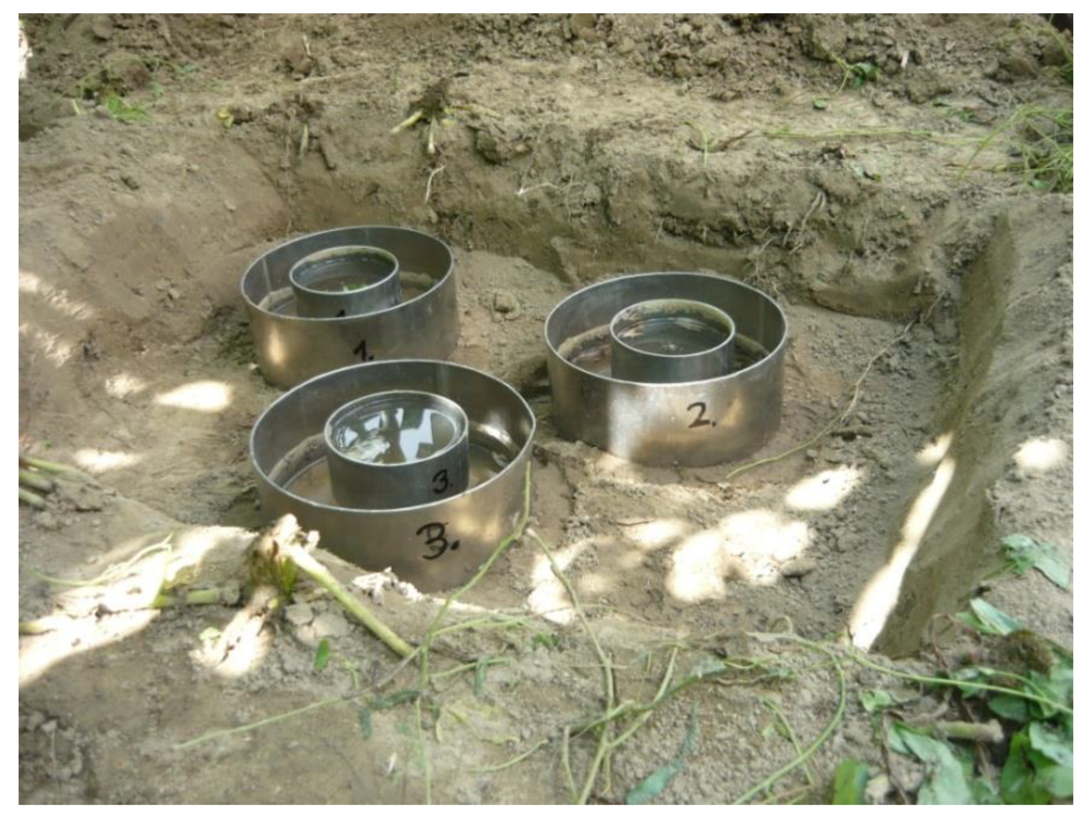
2.3. Field Measurement and Soil Sampling

The research was conducted on arable lands during the agricultural season from 2012 to 2015. The field soil tests were conducted at 16 measurement-control points (up to a depth of 150 cm) in Wojnowice (2 points), Bojanów (2 points), Owsiszcze (6 points), Strzybnik (2 points), and Tworków (4 points). Three to five genetic levels were identified for each soil profile.
The soil infiltration was measured in situ, at depths of 10 cm (topsoil) and 35 cm (subsoil), using a double-ring infiltrometer (DRI) method (Figure 2). The DRI comprised an inner ring (9.5 cm diameter) and outer ring (19.5 cm diameter) inserted into the ground at a depth of 10 cm. The DRI was inserted by using a falling weight-type hammer striking on a wooden plank placed uniformly on top of the ring, and without undue disturbance to the soil surface. Each ring of the DRI was filled with a constant head of water level, and the outer ring helped when checking the lateral flow from the inside ring, so as to better estimate the infiltration, reducing losses. The Ks value was estimated when the water flow rate inside the inner ring reached a steady state [1], which in the case of the studied soils, lasted approximately 3–4 h. The infiltration rate was calculated for the respective time intervals ΔT as follows [41]:
i = 864   ·   4   ·   V   3.14   ·   D r 2   ·   Δ T   ( m · day 1 )
where V is the volume of water (cm3) added to the inner ring at time ΔT (s), and Dr is the diameter of the inner ring (cm2).
For steady infiltration (as a constant value for the soil), the Land and Water Development Division [42] developed infiltration classes, as follows: very slow—<0.024 m·day−1; slow—0.024 ÷ 0.12 m·day−1; moderately slow—0.12 ÷ 0.48 m·day−1; moderate—0.48 ÷ 1.56 m·day−1; moderately rapid—1.56 ÷ 4.20 m·day−1; rapid—4.20 ÷ 5.81 m·day−1; and very rapid—>5.81 m·day−1.
Undisturbed soil samples were taken from each genetic horizon, using cylinders with a volume of 100 cm3 (three replicates). In addition, approximately 1.0 kg of disturbed soil from each genetic horizon was used to determine the soil texture, and other laboratory analyses were performed.

2.4. Laboratory Analysis

The properties of the collected soil samples were determined as follows.
  • The soil texture was determined using the Bouyoucose-Casagrande areometric method, based on a measurement of the density of the soil suspension during progressive sedimentation, and a sieving method to fractionate the sand. The contents of the particle size classes (sand, 2.0–0.05 mm; silt, 0.05–0.002 mm; and clay, <0.002 mm) were determined according to the Soil Taxonomy system from the United States Department of Agriculture [43].
  • The soil bulk density (BD) was determined based on the gravimetric method, based on cylinders (100 cm3) for determining the mass of the dry soil per volume. The weight of each soil core was determined after drying in an oven at 105 °C for approximately 18–24 h. The dry bulk density for each core sample was then calculated as follows [44]:
    B D = M s V t   ( g · cm 3 )
In the above, Ms is the mass of the dry soil weight (g), and Vt is the volume of the total soil sample (cm3).
  • The soil water retention was investigated based on determining the soil suction using ceramic plates in a 5/15 bar pressure plate extractor. The pressure plate equipment used in this study was manufactured by the American Soil Moisture Equipment Corporation. In engineering practice, the soil suction is usually calculated in units of pF, as follows:
    pF = log   h   ( )
Here, h is soil suction pressure (in cm H2O).
In the laboratory, the soil water potentials were measured at 300 cm H2O ≈ 33 kPa ≈ 2.5 pF (representing the field capacity) and 15,000 cm H2O ≈ 1500 kPa ≈ 4.2 pF (representing the permanent wilting point) [45]. The soil volumetric water content (θV) at pF = 2.5 and 4.2 was determined based on the gravimetric method. In particular, it was calculated as the ratio of the amount of water in the soil sample to the dry weight of the soil, after drying in an oven at 105 °C for approximately 18–24 h, as follows [44]:
θ V = V H 2 O V t   ( cm 3 · cm 3 )
In the above, VH2O is the volume of water in the soil sample (cm3), and Vt is the volume of the total soil sample (cm3).
  • The Ks was measured under laboratory conditions using a laboratory permeameter (Figure 3) and using the Darcy’s law [46] with constant head method (Equation (6)) and falling head method (Equation (7) on undisturbed soil samples for three replications. The constant method can be used with virtually any soil, apart from poorly permeable soils such as clay, whereas the falling-head method is used to measure low-permeability soils, such as f.i. clay or peat samples [47,48]. The soil samples were placed in the laboratory permeameter and then saturated in water for 2–3 days. For the purpose of this study, a permeameter produced by the Eijkelkamp with a closed or open system and 25 holders was used. The Ks was calculated using the Darcy’s [46] equation, as follows:
    V = K   · i   · A   · t
Here, explanations below;
Determining Ks using the constant head method was calculated from the following equation:
  Ks = V   · L A   · t   · h
Here, V is the volume of water flowing through the sample (cm3); K is the permeability coefficient or ‘Ks’ (cm·day1 or m·day1); h is the water level difference inside and outside ringholder or sample cylinder (cm); L is the length of the soil sample (cm); i is the permeability rise gradient or h/L (–); A is the cross-sectional area of the sample (m2); and t is the time used for flow through of water volume (day). During measuring the following parameters have been determined: L and A—constants, depending on the type of sample ring used; V—volume measured in the burette (1 mL = 1 cm3); t—length of time lapse; h—calculated with the water levels measured with the water level meter.
Determining Ks using the falling head method was calculated from the following equation:
K s = a   · L A   · ( t 2 t 1 )   · l n h 1 h 2 + x   · a   · L A   ·   ( h 1   ·   h 2 )
Here, Ks is the permeability coefficient (cm·day1 or m·day−1); h is the water level difference inside and outside ringholder or sample cylinder (cm) h1 and h2 water level difference inside and outside the ringholder at respectively t1(start) and t2 (end); A is the surface of a cross-section of the sample (cm2); L is the length of the soil sample (cm); t is the time between beginning and end of the measuring t2t1 (day); a is the cross-section surface of a ringholder or sample cylinder (cm2) for a sample cylinder applies A = a; x is the evaporation factor (literature value): 0.0864 cm·day−1 or 0.000864 m·day−1.
The permeability of the soil is also determined by viscosity of the soil solution. Viscosity depends on the temperature. The laboratory water temperature varies from 18 to 22 °C, whereas the average groundwater temperature is 10 °C. Therefore, for certain applications the permeability will have to be corrected for the viscosity of the soil solution (usually water). The Ks for viscosity was corrected using the following equation [49]:
K 10 = K T   ·   h T h 10
Here, K10 is the corrected Ks at 10 °C (cm·day−1 or m·day−1); KT is the Ks at the applied temperature (cm·day−1 or m·day−1); h10 is the dynamic viscosity of water at 10 °C (Pa·s); hT is the dynamic viscosity of water at T °C (Pa·s).
The soil classification was established according to the Polish Soil Classification [50], World Reference Base for Soil Resources (FAO and International Union of Soil Sciences (IUSS) Working Group World Reference Base (WRB), [51]), and USDA soil taxonomy (Soil Survey Staff, [43]).

2.5. Rosetta Description

The Ks values were calculated using the published neural network program Rosetta, with hierarchical PTFs based on five levels of input data [5]. The first level (PTF-1) used soil textural classes based on a lookup table providing parameter means for each USDA textural class. The second level (PTF-2) used the sand, silt, and clay percentages as inputs, and in contrast to PTF-1, provided hydraulic parameters that varied continuously with the texture. The third level (PTF-3) included the predictors used in the level PTF-2, along with the soil dry-bulk density. The fourth level (PTF-4) used PTF-3 and the soil volumetric water content (θ) at a water suction of 33 kPa (2.5 pF). The last level (PTF-5) comprised all of the other parameters, plus the θ value at a water suction of 1500 kPa (4.2 pF) [38,52]. The necessary input data for the Rosetta program (e.g., % soil texture group and bulk density) were determined based on the laboratory analyses of soil samples from the different soil horizons (Table 2, Table 3 and Table 4).
In the Rosetta program, the relationship between θ and the water suction (h), i.e., the water retention θ(h), as well as Ks, are described using the well-known Mualem–van Genuchten equations [53] and are given as follows:
θ ( h ) = θ r + θ s θ r   [ 1 + ( α | h | n ] m
K ( h ) = K s { 1 ( α   · h ) n 1 [ 1 + ( α   · h ) n ) ] m } 2 [ 1 + ( α   · h ) n ] m / 2
In the above, θ(h) is the soil volumetric water content (cm3∙cm−3) at suction h (cm H2O); θs and θr are the saturated and residual water contents (cm3∙cm−3) at h = 0 and 15,000 cm H2O, respectively; α (>0 in cm−1) is related to the inverse of the air entry suction; n (>1) is a measure of the pore-size distribution, and m = 1 − 1/n; and Ks is the saturated hydraulic conductivity (m∙day−1), as mentioned above.

2.6. Statistical Analysis and Model Performance Evaluation

The data set comprised the analytical results from the soil samples collected from the 16 soil pits. For the statistical analysis, the procedures provided by the program Statistica PL Version 12.5 were used, with a 5% significance level. The minimum and maximum values were determined for each physical parameter of the soil, and the arithmetic mean, median, standard deviation (SD), and coefficient of variation (CV) were computed. Moreover, a Spearman correlation test was conducted for the dataset. The correlation strength and direction of the relationship between two variables were determined based on Spearman’s rank correlation coefficient (rho), which takes values from −1 to 1. A positive sign of the coefficient indicated the existence of a positive correlation, and vice versa. The closer the values were to −1 and 1, the stronger the correlation. When rho = 0, there was no correlation between the examined variables [54]. This statistical method was chosen after finding that most data were not normally distributed (Shapiro-Wilk test). All of data are presented in the tables and graphs, i.e., to produce a visual image that is helpful in interpreting the results.
Based on the available soil data in this study, five widely used PTFs were selected to assess their respective performances in estimating Ks, via comparison with the measured Ks values (via the DRI) for the soil cores collected in the field (using a laboratory permeameter). The calculated values of Ks obtained using Rosetta were compared to the corresponding measured values and evaluated using two statistical parameters: root-mean-square deviation (RMSD) and Nash–Sutcliffe efficiency (NSE). The RMSD gives the mean difference between the measured and calculated values of Ks, and is calculated as follows [38,55]:
RMSD = 1 n   i = 1 n ( m i p i ) 2
where: mi is the measured value of Ks, and pi is the corresponding (predicted) value of Ks as obtained using the Rosetta program.
The RMSD values are always non-negative and should be as low as possible; RMSD = 0 indicates a perfect fit of the model to the measurement data.
The NSE compares measured and predicted values (here, for Ks), and is given as follows [56]:
N S E = 1 [ i = 1 n ( m i p i ) 2 i = 1 n ( m i m ¯ i ) 2 ]
In the above, n is the number of observations, mi and pi are the measured and predicted values of Ks, respectively, and m ¯ i is the mean of the measured Ks values.
The NSE values range from −∞ to 1. A value of NSE = 1 corresponded to a perfect match of calculated values to the measured values of Ks. The ‘efficiency NSE’ = 0 indicated that the calculations of Ks using the Rosetta program were as accurate as the mean of the measured data; in contrast, an efficiency NSE < 0 occurred when the measured mean was a better predictor than the model or, in other words, when the residual variance, as described by the numerator in the equation above, was larger than the data variance described by the denominator.

3. Results and Discussion

According to the PTG [50], FAO and IUSS Working Group WRB [52], and USDA soil taxonomy [43], the examined soils were classified as follows.
  • Order 3: Brown forest soils (brown earths, PTG—Polish: Gleby brunatnoziemne; WRB: Cambisols; USDA: Inceptisols—Udepts), Type 3.1. ‘Euthrophic brown soils’ (PTG—Polish: Gleby brunatne eutroficzne; WRB: Haplic Cambisol, Haplic, Stagnic, Endogleyic, or Vertic Cambisol (Eutric); USDA: Typic or Humic or Aquic or Oxyaquic or Vertic Eutrudepts)—occurred in Strzybnik.
  • Order 5: Brown forest podzolic soils (Soil lessivé) (PTG—Polish: Gleby płowoziemne; WRB: Luvisols, Albeluvisols; USDA: Alfisols—Aqualfs, Udalfs), Type 5.2. ‘Streak brown forest podzolic soils’ (PTG—Polish: Gleby płowe zaciekowe; WRB: Haplic, Stagnic, Gleyic, Cambic Albeluvisol; USDA: Typic, Arenic, Aquic, Oxyaquic, Haplic, Glossaqiuc, or Vertic Glossudalfs)—occurred in Wojnowice, Bojanów and Owsiszcze.
  • Order 7: Chernozemic soils (PTG—Polish: Gleby czarnoziemne; WRB: Chernozems, Phaeozems; USDA: Mollisols—Aquolls, Udolls), Type 7.4. ‘Chernoziemic fluvisols’ (PTG—Polish: Mady czarnoziemne; WRB: Mollic Fluvisol, Endofluvic Phaeozem; USDA: Fluvaquentic Endoaquolls)—occurred in Tworków.
As shown in Table 2 and Figure 4, the examined soils are heterogeneous in terms of their textures. Seven textural classes are observed in the examined soil profiles: silt loam (SiL; n = 42), sandy loam (SL; n = 10), loam (L; n = 6), clay (C; n = 3), sandy clay loam (SCL; n = 3), clay loam (CL; n = 2), and silty clay loam (SiCL; n = 2). The silt loam is the predominant soil texture. The SD values (Table 3 and Table 4) for most soil properties are large, indicating moderate to strong variability; this is not uncommon for soils [12,57,58]. Typically, the CV values are < 45%, indicating the mean variability of the measurement data. The highest CV values are observed for sand (57.0%) and clay (57.2%). The sand content in the soil profiles is between 11% and 76%, the silt content is between 16% and 72%, and the clay content is between 8% and 65% (Table 2 and Table 4). The high swelling-clay content could be a cause of the poor water flow through the samples, as well as a consequence of abnormal Ks results [59].
With regard to the surface soil horizons (n = 32), the mean soil bulk density (ρb) is 1.55 g∙cm−3, whereas that for overall depths is 1.60 g∙cm−3 (Table 3 and Table 4). The soil volumetric water contents at the matric potentials of 33 kPa (2.5 pF) and 1500 kPa (4.2 pF) in both cases have similar mean values (0.350/0.351 cm3∙cm−3 and 0.152/0.155 cm3∙cm−3, respectively).
Higher values of Ks are found in the upper horizons of the tested soils, owing to the significant macroporosity caused by plant roots, reconsolidation [60], and annual loosening from agrotechnical works and alternating soil freezing and thawing [61]. In addition, zoogenic channels (especially earthworm channels) and plant residues increase soil permeability [62]. For these reasons, the samples taken from arable and sub-arable horizons are less dense than those from lower horizons; the latter are also subject to self-compacting (Table 2, Table 3 and Table 4).
Table 5 presents descriptive statistics concerning the values of Ks for the topsoils and subsoils (n = 32), as obtained from in situ and laboratory measurements, and as estimated with the use of the PTF models in the Rosetta program (variant 1). In contrast, Table 6 presents statistical measures considering the Ks values of all of the soil horizons (n = 68), but excludes the in situ tests not conducted on larger and deeper horizons, for practical reasons (variant 2).
In variant 1, the characteristic values of Ks (maximum, mean, and median values) as obtained from the in situ measurements are approximately four times higher than the Ks values obtained from the laboratory measurements. Such large discrepancies between the results obtained from both direct methods result from the manner of conducting the measurements; in particular, small-volume soil samples, which do not allow for the inclusion of all of the factors influencing the soil permeability, were taken for the laboratory tests. The mean Ks value obtained from the in situ measurements, i.e., 0.85 m·day−1, is four times higher than those estimated by PTF-1 and PTF-2, almost half lower than that obtained from PTF-3, and twice as high as the values obtained from PTF-4 and PTF-5. In addition, the median value from the in situ tests (0.40 m·day−1) is from 1.2 to 2.2 times higher than the values obtained from the four PTF models—the exception is model PTF-3, whose median value is four times higher than that from the in situ tests. The maximum and mean values of the Ks values obtained from laboratory tests, compared to those from the in situ method, are usually more similar to those obtained from the PTF models (Table 5). The mean Ks values obtained from the in situ measurements and PTF-3 indicate the mean class, whereas the results obtained from laboratory measurements and the other four PTF models indicate a moderately slow basic infiltration class [42].
Most of the subsurface horizons are characterised by low Ks values, usually not exceeding 0.50 m·day−1. In variant 2, covering the analysis of all soil horizons, the mean value of Ks from the laboratory measurements (0.21 m·day−1) is very close to the results obtained from the PTF-1 and PTF-2 models, almost six times lower than the Ks value from PTF-3, and three times lower than the values estimated by PTF-4 and PTF-5 (Table 6). The mean Ks values obtained from the laboratory measurements and PTF-1, PTF-2, and PTF-3 indicate the moderate class, whereas the results obtained from the other three PTF models indicate a moderately slow basic infiltration class [42].
Regardless of the amount of data taken for analysis (n = 32 or 68), the values of Ks are usually characterised by high or very high random variability (CV = 26.1–230.7%), not only in comparison to the other soil hydrophysical properties, but also compared to the methods used to determine Ks, i.e., field, laboratory, and PTF tests (Table 5 and Table 6, Figure 5). This regularity has been described in various other studies, for example, Rezaei et al. [63]. As reported by Merdun et al. [64] and García-Gutiérrez et al. [65], the high spatial variability between the soil horizons with regard to Ks are the result of the soil heterogeneity, which hampers the prediction of Ks using mathematical models.
The Ks values obtained from the laboratory measurements are statistically significant (p < 0.05), negatively correlated with the clay fraction and density, and positively correlated with the sand fraction (Table 7). Similar observations were noted by Zhao et al. [13], who conducted studies on the Loess Plateau of China. The interdependence of Ks values and soil textures were well documented by Hillel [66], García-Gutiérrez et al. [65], and other researchers [3]. In the case of in situ measurements, the soil hydraulic conductivity is only significantly positively correlated with the sand fraction (rho = 0.29). The PTF-1 model is significantly positively correlated with the soil density, but negatively correlated with the clay fraction and soil volumetric water content (θ) at water suctions of 33 and 1500 kPa (2.5 pF and 4.2 pF). The PTF-2 and PTF-3 models show a significantly positive correlation with the sand fraction and negative correlations with the clay fraction and soil volumetric water content (θ) at 2.5 and 4.2 pF. The PTF-4 and PTF-5 models are significantly positively correlated with the sand fraction, and are negatively correlated with the dust fraction (Table 7).
No significant correlations were detected between the Ks values obtained from the in situ measurements and the PTF models. However, with the exception of the PTF-1 model, the Ks values from the laboratory tests as estimated by the four PTF models are positively correlated (Table 7). For these reasons, only the linear correlations between the values obtained from the laboratory tests and PTF models are presented in Figure 6a–e.
In general, the matching of the Ks results obtained from the direct in situ measurements with the results estimated by the Rosetta PTFs is poorer than that obtained from the laboratory measurements and estimated by the Rosetta PTFs. This is confirmed by the RMSD values, which range from 1.40 to 1.64 in the first case, whereas in the second case, they range from 0.19 to 1.58. In addition, the values of the coefficient of determination (R2), which indicates the extent to which the model explains the gathered measurement data, are usually much higher when comparing the data obtained from the laboratory tests and that from the PTF models (Table 8).
The RMSD values of the Ks results obtained from the laboratory measurements and estimated with PTFs reveal the best match for the case of the PTF-2 model. The NSE and R2 values are the best in this case (Table 8), indicating that the granulometric composition (% of sand, silt, and clay) in the PTF-2 model has the greatest influence on the water permeability of the soils.

4. Conclusions

The search for alternatives to labour-intensive and cost-intensive in situ tests and laboratory methods for determining the value of Ks, at a time of global climate change, seems to be a priority. The increased frequency of periods with excesses and scarcities of water will require the greater use of soil irrigation and drainage facilities, and the modelling of surface runoff and erosion phenomena in land-formed areas. Correspondingly, knowledge regarding soil permeability is required for all technical and non-technical activities.
In general, when using a descriptive comparative analysis, it is difficult to show a significant relationship between Ks values from in situ tests and the diverse hydrophysical properties of arable soils, which are subject to cyclic loosening, reconsolidation, and/or freezing and thawing. The high sensitivity of this physical parameter to biotic and abiotic factors, especially in the soil upper horizons, hampered a satisfactory adjustment to the Ks values obtained from the PTF models. Therefore, in situ tests, although difficult and time-consuming, should continue to be conducted to obtain a reliable measurement database that is free of errors resulting from the soil type variability, and that considers the influences of fauna and flora on the physical properties of soil. This is of particular importance for the modelling of surface runoff and erosion processes and design of surface irrigation systems (e.g., sprinklers), where only 40–50 cm of the upper horizon of the soil is wetted, and the technical parameters of the corresponding drainage facilities are highly dependent on soil permeability.
The in situ measurements of Ks are significantly correlated only with the laboratory tests; nevertheless, the values obtained in situ are much higher, and are influenced by a number of factors, including those of a methodological nature (e.g., the larger diameter of the measuring cylinder). In contrast, the laboratory measurements show a significant correlation with the Ks values estimated using the models PTF-2 to PTF-5. The best match is found (based on the RMSD, NSE, and R2 values) when using the PTF-2 model in the Rosetta program. This means that the most reliable Ks values can be obtained from the percentages of the sand, dust, and clay fractions. Therefore, there is a rational alternative, in the form of the PTF, for the costly and labour-intensive determinations of Ks conducted in the laboratory. The use of the PTF-2 model allows for the determination of the hydraulic conductivity of deeper soil horizons, where the variability of the hydrophysical properties is lower and there are large methodological limitations in conducting field work or difficulties in taking intact structural samples for laboratory tests. This type of solution can be used to collect data for designing subsurface drainage and irrigation facilities, some of the technical parameters of which are determined by the Ks values.
In conclusion, the research results confirmed the remarkable difference between the performance of PTFs in the Rosetta and the Ks results obtained from field or laboratory measurements. The study thus provided evidence that the Ks values obtained from local dataset give better results performances in predicting the soil saturated hydraulic conductivity, compared to PTFs in the Rosetta derived from large datasets, which in turn confirm the limitation of applying PTFs developed from one region to other regions.

Author Contributions

Conceptualization, Ł.B., A.B. and T.K.; methodology, Ł.B., A.B. and T.K.; software, Ł.B.; validation, Ł.B.; formal analysis, Ł.B.; investigation, Ł.B., A.B. and T.K.; resources, Ł.B., A.B. and T.K.; data curation, Ł.B., A.B. and T.K.; writing—original draft preparation, Ł.B., A.B. and T.K.; writing—review and editing, Ł.B. and T.K.; visualization, Ł.B.; supervision, T.K.; project administration, Ł.B; funding acquisition, Ł.B., A.B. and T.K. All authors have read and agreed to the published version of the manuscript.

Funding

This research was funded by the Department of Land Reclamation and Environmental Development, Faculty of Environmental Engineering and Land Surveying, University of Agriculture in Krakow.

Institutional Review Board Statement

Not applicable.

Informed Consent Statement

Not applicable.

Data Availability Statement

Not applicable.

Acknowledgments

The authors would like to acknowledge the authorities of the Agro-Industrial Company ‘AGROMAX’ in Racibórz for providing agricultural areas and agricultural equipment for the field study.

Conflicts of Interest

The authors declare no conflict of interest.

References

  1. Islam, A.; Mailapalli, D.R.; Behera, A. Evaluation of Saturated Hydraulic Conductivity Methods for Different Land Uses. Indian J. Ecol. 2017, 44, 456–466. [Google Scholar]
  2. Kanso, T.; Tedolidi, D.; Gromaire, M.-C.; Rameier, D.; Saad, M.; Chebbo, G. Horizontal and vertical variability of soil hydraulic properties in roadside sustainable drainage systems (SuDS)—Nature and Implications for Hydrological Performance Evaluation. Water 2018, 10, 987. [Google Scholar] [CrossRef] [Green Version]
  3. Ottoni, M.V.; Ottoni Filho, T.B.; Lopes-Assad, M.L.R.; Rotunno Filho, O.C. Pedotransfer functions for saturated hydraulic conductivity using a database with temperate and tropical climate soils. J. Hydrol. 2019, 575, 1345–1358. [Google Scholar] [CrossRef]
  4. Jabro, J.D. Estimation of saturated hydraulic conductivity of soils from particle-size distribution and bulk-density data. Trans. ASAE 1992, 35, 557–560. [Google Scholar] [CrossRef]
  5. Schaap, M.G.; Leij, F.J.; van Genuchten, M.T. ROSETTA: A computer program for estimating soil hydraulic parameters with hierarchical pedotransfer functions. J. Hydrol. 2001, 251, 163–176. [Google Scholar] [CrossRef]
  6. Li, Y.; Chen, D.; White, R.E.; Zhu, A.; Zhang, J. Estimating soil hydraulic properties of Fengqiu County soils in the North China plain using pedo-transfer functions. Geoderma 2007, 138, 261–271. [Google Scholar] [CrossRef]
  7. Jarvis, N.; Koestel, J.; Messing, I.; Moeys, J.; Lindahl, A. Influence of soil, land use and climatic factors on the hydraulic conductivity of soil. Hydrol. Earth Syst. Sci. 2013, 17, 5185–5195. [Google Scholar] [CrossRef] [Green Version]
  8. Papanicolaou, A.N.; Elhakeem, M.; Wilson, C.G.; Burras, C.L.; West, L.T.; Lin, H.; Clark, B.; Oneal, B.E. Spatial variability of saturated hydraulic conductivity at the hillslope scale: Understanding the role of land management and erosional effect. Geoderma 2015, 243–244, 58–68. [Google Scholar] [CrossRef]
  9. Kruk, E. Impact of the Technological Path on Some Soil Properties on Loess Slope. J. Ecol. Eng. 2019, 20, 169–176. [Google Scholar] [CrossRef]
  10. Borek, Ł.; Bogdał, A.; Ostrowski, K. The effect of subsoiling on change of compaction and water permealility of silt loam. Annu. Set Environ. Prot. 2018, 20, 538–557. Available online: http://towarzystwo.ros.edu.pl/images/roczniki/2018/030_ROS_V20_R2018.pdf, (accessed on 5 December 2020).
  11. Lauffenburger, Z.H.; Gurdak, J.J.; Hobza, C.; Woodward, D.; Wolf, C. Irrigated agriculture and future climate change effects on groundwater recharge, northern High Plains aquifer, USA. Agric. Water Manag. 2018, 204, 69–80. [Google Scholar] [CrossRef] [Green Version]
  12. Gamie, R.; De Smedt, F. Experimental and statistical study of saturated hydraulic conductivity and relations with other soil properties of a desert soil. Eur. J. Soil Sci. 2018, 69, 256–264. [Google Scholar] [CrossRef] [Green Version]
  13. Zhao, C.; Shao, M.; Jia, X.; Nasir, M.; Zhang, C. Using pedotransfer functions to estimate soil hydraulic conductivity in the Loess Plateau of China. CATENA 2016, 143, 1–6. [Google Scholar] [CrossRef]
  14. Jačka, L.; Pavlásek, J.; Kuráž, V.; Pech, P. A comparison of three measuring methods for estimating the saturated hydraulic conductivity in the shallow subsurface layer of mountain podzols. Geoderma 2014, 219–220, 82–88. [Google Scholar] [CrossRef]
  15. Twarakavi, N.K.C.; Simunek, J.J.; Schaap, M.G. Development of pedotransfer functions for estimation of soil hydraulic parameters using support vector machines. Soil Sci. Soc. Am. J. 2009, 73, 1443–1452. [Google Scholar] [CrossRef] [Green Version]
  16. Bouma, J. Using soil survey data for quantitative land evaluation. Adv. Soil Sci. 1989, 9, 177–213. [Google Scholar] [CrossRef]
  17. Deb, S.K.; Shukla, M.K. Variability of hydraulic conductivity due to multiple factors. Am. J. Environ. Sci. 2012, 8, 489–502. [Google Scholar] [CrossRef] [Green Version]
  18. Gunarathna, M.; Sakai, K.; Nakandakari, T.; Momii, K.; Kumari, M. Machine learning approaches to develop pedotransfer functions for tropical Sri Lankan soils. Water 2019, 11, 1940. [Google Scholar] [CrossRef] [Green Version]
  19. Givi, J.; Prasher, S.O.; Patel, R.M. Evaluation of pedotransfer functions in predicting the soil water contents at field capacity and wilting point. Agric. Water Manag. 2004, 70, 83–96. [Google Scholar] [CrossRef]
  20. Borek, Ł.; Bogdał, A. Soil wetar retention of the Odra River alluvial soils (Poland): Estimating parameters by RETC model and laboratory measurements. Appl. Ecol. Environ. Res. 2018, 16, 4681–4699. Available online: http://www.aloki.hu/pdf/1604_46814699.pdf (accessed on 11 December 2020). [CrossRef]
  21. Wang, J.-P.; Zhuang, P.-Z.; Luan, J.-Y.; Liu, T.-H.; Tan, Y.-R.; Zhang, J. Estimation of unsaturated hydraulic conductivity of granular soils from particle size parameters. Water 2019, 11, 1826. [Google Scholar] [CrossRef] [Green Version]
  22. Zhang, Y.; Schaap, M.G. Estimation of saturated hydraulic conductivity with pedotransfer functions: A review. J. Hydrol. 2019, 575, 1011–1030. [Google Scholar] [CrossRef]
  23. Ahuja, L.R.; Cassel, D.K.; Bruce, R.R.; Barnes, B.B. Evaluation of spatial distribution of hydraulic conductivity using effective porosity data. Soil Sci. 1989, 148, 404–411. [Google Scholar] [CrossRef]
  24. Rawls, W.J.D.; Gimenez, D.; Grossman, R. Use of soil texture, bulk density and slope of the water retention curve to predict saturated hydraulic conductivity. Trans. ASAE 1998, 41, 983–988. [Google Scholar] [CrossRef]
  25. Timlin, D.J.; Ahuja, L.R.; Pachepsky, Y.; Williams, R.D.; Gimenez, D.; Rawls, W. Use of Brooks-Corey parameters to improve estimates of saturated conductivity from effective porosity. Soil Sci. Soc. Am. J. 1999, 63, 1086–1092. [Google Scholar] [CrossRef] [Green Version]
  26. Suleiman, A.A.; Ritchie, J.T. Estimating saturated hydraulic conductivity from soil porosity. Trans. ASAE 2001, 44, 235–339. [Google Scholar] [CrossRef]
  27. Cosby, B.J.; Hornberger, G.M.; Clapp, R.B.; Ginn, T.R. A statistical exploration of the relationships of soil moisture characteristics to the physical properties of soils. Water Resour. Res. 1984, 20, 682–690. [Google Scholar] [CrossRef] [Green Version]
  28. Wösten, J.H.M.; Lilly, A.; Nemes, A.; Le Bas, C. Development and use of a database of hydraulic properties of European soils. Geoderma 1999, 90, 169–185. [Google Scholar] [CrossRef]
  29. Saxton, K.E.; Rawls, W.J. Soil water characteristic estimates by texture and organic matter for hydrologic solutions. Soil Sci. Soc. Am. J. 2006, 70, 1569–1578. [Google Scholar] [CrossRef] [Green Version]
  30. Weynants, M.; Vereecken, H.; Javaux, M. Revisiting vereecken pedotransfer functions: Introducing a closed-form hydraulic model. Vadose Zone J. 2009, 8, 86–95. [Google Scholar] [CrossRef] [Green Version]
  31. Zhang, Y.; Schaap, M.G. Weighted recalibration of the rosetta pedotransfer model with improved estimates of hydraulic parameter distributions and summary statistics (Rosetta 3). J. Hydrol. 2017, 547, 39–53. [Google Scholar] [CrossRef] [Green Version]
  32. Araya, S.N.; Ghezzehei, T.A. Using machine learning for prediction of saturated hydraulic conductivity and its sensitivity to soil structural perturbations. Water Resour. Res. 2019, 55, 5715–5737. [Google Scholar] [CrossRef]
  33. Puckett, W.E.; Dane, J.H.; Hajek, B. Physical and Mineralogical Data to Determine Soil Hydraulic Properties†. Soil Sci. Soc. Am. J. 1985, 49, 831–836. [Google Scholar] [CrossRef]
  34. Campbell, G.S. Soil Physics with BASIC: Transport Models for Soil-Plant Systems; Elsevier Scientific: New York, NY, USA, 1985. [Google Scholar]
  35. Smettem, K.R.J.; Bristow, K.L. Obtaining soil hydraulic properties for water balance and leaching models from survey data. 2. Hydraulic conductivity. Aust. J. Agric. Res. 1999, 50, 1259–1262. [Google Scholar] [CrossRef]
  36. Saxton, K.E.; Rawls, W.J.; Romberger, J.S.; Papendick, R. Estimating general soil-water characteristics from texture. Soil Sci. Soc. Am. J. 1986, 5, 1031–1036. [Google Scholar] [CrossRef]
  37. Zhang, Y.; Schaap, M.G.; Zha, Y. A highresolution global map of soil hydraulic properties produced by a hierarchical parameterization of a physically based water retention model. Water Resour. Res. 2018, 54, 9774–9790. [Google Scholar] [CrossRef] [Green Version]
  38. Alvarez-Acosta, C.; Lascano, R.J.; Stroosnijder, L. Test of the ROSETTA pedotransfer function for saturated hydraulic conductivity. Open J. Soil Sci. 2012, 2, 203–212. [Google Scholar] [CrossRef] [Green Version]
  39. Kondracki, J. Regional Geography of Poland; PWN: Warszawa, Poland, 2011; 440p, ISBN 9788301160227. (In Polish) [Google Scholar]
  40. Skowera, B. Changes of hydrothermal conditions in the Polish area (1971–2010). Fragm. Agron. 2014, 31, 74–87. (In Polish). Available online: https://pta.up.poznan.pl/pdf/2014/FA%2031(2)_2014_skowera_nowa_wersja.pdf (accessed on 3 December 2020).
  41. Gulliver, J.S.; Anderson, J.L. (Eds.) Assessment of Stormwater Best Management Practices; Report of Stormwater Management Practice Assessment Project; University of Minnesota: Minneapolis, MN, USA, 2008; 599p. [Google Scholar]
  42. FAO. Land and Water Development Division; FAO: Rome, Italy, 1971. [Google Scholar]
  43. Soil Survey Staff. Soil Taxonomy: A Basic System of Soil Classification for Making and Interpreting Soil Surveys, 2nd ed.; Handbook; United States Department of Agriculture (USDA), Natural Resources Conservation Service: Washington, DC, USA, 1999; 886p. Available online: https://www.nrcs.usda.gov/Internet/FSE_DOCUMENTS/nrcs142p2_051232.pdf (accessed on 13 December 2020).
  44. Phogat, V.K.; Tomar, V.S.; Dahyia, R. Soil Physical Properties (Chapter 6). In Soil Science: An Introduction, 1st ed.; Rattan, R.K., Katyal, J.C., Dwivedi, B.S., Sarkar, A.K., Bhattachatyya, T., Tarafdar, J.C., Kukal, S.S., Eds.; Indian Society of Soil Science: New Delhi, India, 2015; pp. 135–171. [Google Scholar]
  45. Mocek, A.; Drzymała, S. Genesis, Analysis and Classification of Soils; Wyd. UP: Poznań, Poland, 2010; 418p. (In Polish) [Google Scholar]
  46. Darcy, H. Les Fontaines Publiques de la Ville de Dijon [The Public Fountains of the City of Dijon]; Dalmont: Paris, France, 1856. (In France) [Google Scholar]
  47. Klute, A.; Dinauer, R.C.; Page, A.L.; Miller, R.H.; Keeney, D.R. Methods of Soil Analysis. Part 1. Physical a Mineralogical Methods; SSSA Book Series No 5; Soil Science Society of America: Madison, WI, USA, 1986; p. 1358. ISBN 978-0891188117. [Google Scholar]
  48. Eijkelkamp. Laboratory Permeameter. Operating Instructions. 2017. Available online: https://en.eijkelkamp.com/products/laboratory-equipment/permeameter-closed-system-25-holders-73766.html;https://en.eijkelkamp.com/products/laboratory-equipment/set-for-pf-determination-with-ceramic-plates.html (accessed on 13 December 2020).
  49. Wit, K.E. Meting van de Doorlatendheid in Ongeroerde Monsters; Rapport 17; ICW: Wageningen, The Netherlands, 1963. [Google Scholar]
  50. PTG. Polish Soil Classification, 5th ed.; Soil Science Annual; 2011; Volume 62, p. 193. Available online: http://ssa.ptg.sggw.pl/en/artykul/2810/polish-soil-classification-fifth-edition (accessed on 13 December 2020). (In Polish).
  51. FAO; IUSS Working Group WRB. World Reference Base for Soil Resources 2014. International Soil Classification System for Naming Soils and Creating Legends for Soil Maps; World Soil Resources Reports, No. 106; FAO: Rome, Italy, 2015; p. 203. ISBN 978-92-5-108369-7. [Google Scholar]
  52. Schaap, M.G.; Leij, F.J.; van Genuchten, M.T. Neural network analysis for hierarchical prediction of soil water retention and saturated hydraulic conductivity. Soil Sci. Soc. Am. J. 1998, 62, 847–855. [Google Scholar] [CrossRef]
  53. Schaap, M.G.; van Genuchten, M.T. A modified Mualem-van Genuchten formulation for improved description of the hydraulic conductivity near saturation. Vadose Zone J. 2006, 5, 27–34. [Google Scholar] [CrossRef] [Green Version]
  54. Rumsey, D.J. Statistics for Dummies, 2nd ed.; 2016; 408p. Available online: https://www.gettextbooks.com/author/Deborah_J_Rumsey (accessed on 19 December 2020).
  55. Zhang, X.; Zhu, J.; Wendroth, O.; Matocha, C.; Edwards, D. Effect of macroporosity on pedotransfer function estimates at the field scale. Vadose Zone J. 2019, 18, 180151. [Google Scholar] [CrossRef]
  56. Nash, J.E.; Sutcliffe, J.V. River Flow Forecasting through Conceptual Model. Part 1—A Discussion of Principles. J. Hydrol. 1970, 10, 282–290. [Google Scholar] [CrossRef]
  57. Mulla, D.J.; Mc Bratney, A.B. Soil spatial variability. In Soil Physics Companion; Warrick, A.W., Ed.; CRC Press: Boca Raton, FL, USA, 2002; pp. 343–373. [Google Scholar]
  58. Borek, Ł. The use of different indicators to evaluate chernozems fluvisols physical quality in the Odra River valley: A case study. Pol. J. Environ. Stud. 2019, 28, 4109–4116. [Google Scholar] [CrossRef]
  59. Rubio, C.M.; Poyatos, R. Applicability of HYDRUS-1D in a Mediterranean mountain area submitted to land use changes. Int. Sch. Res. Not. Soil Sci. 2012, 1–7. Available online: http://downloads.hindawi.com/archive/2012/375842.pdf (accessed on 13 December 2020). [CrossRef] [Green Version]
  60. Gill, S.M. Temporal Variability of Soil Hydraulic Properties under Different Soil Management Practices. 2012. Available online: https://www.researchgate.net/publication/311674921_ (accessed on 20 December 2020).
  61. Pollacco, J.A.P.; Webb, T.; McNeill, S.; Hu, W.; Carrick, S.; Hewitt, A.; Lilburne, L. Saturated hydraulic conductivity model computed from bimodal water retention curves for a range of New Zealand soils. Hydrol. Earth Syst. Sci. 2017, 21, 2725–2737. [Google Scholar] [CrossRef] [Green Version]
  62. Dexter, A.R.; Czyż, E.A.; Gaţe, O.P. Soil structure and the saturated hydraulic conductivity of subsoils. Soil Tillage Res. 2004, 79, 185–189. [Google Scholar] [CrossRef]
  63. Rezaei, M.; Saey, T.; Seuntjens, P.; Joris, I.; Boënne, W.; Van Meirvenne, M.; Cornelis, W. Predicting saturated hydraulic conductivity in a sandy grassland using proximally sensed apparent electrical conductivity. J. Appl. Geophys. 2016, 126, 35–41. [Google Scholar] [CrossRef]
  64. Merdun, H.; Çınar, Ö.; Meral, R.; Apan, M. Comparison of artificial neural network and regression pedotransfer functions for prediction of soil water retention and saturated hydraulic conductivity. Soil Tillage Res. 2006, 90, 108–116. [Google Scholar] [CrossRef]
  65. García-Gutiérrez, C.; Pachepsky, Y.; Martín, M.A. Technical note: Saturated hydraulic conductivity and textural heterogeneity of soils. Hydrol. Earth Syst. Sci. 2018, 22, 3923–3932. [Google Scholar] [CrossRef] [Green Version]
  66. Hillel, D. Fundamentals of Soil Physics; Academic Press: New York, NY, USA, 2013; 413p, ISBN 9780080918709. [Google Scholar]
Figure 1. Location of the study area.
Land 10 00959 g001
Figure 2. The double-ring infiltrometer (DRI) (photo. Ł. Borek).
Land 10 00959 g002
Figure 3. The laboratory permeameter produced by the Eijkelkamp (photo. Ł. Borek).
Land 10 00959 g003
Figure 4. Textural composition of soils investigated.
Land 10 00959 g004
Figure 5. Box plots showing the performance of Ks to different measurement methods.
Land 10 00959 g005
Figure 6. The laboratory measured and predicted saturated hydraulic conductivity Ks for the five pedotransfer function models invistigated (PTF).
Land 10 00959 g006aLand 10 00959 g006b
Table 1. The characteristics of meteorological conditions of the study area.
Year or Multi-YearMonths of the Growing SeasonPeriod
AprMayJunJulAugSepApr–SepJan–Dec
Sum of precipitation totals (mm)
201069204112957578633828
20112769851316217391508
2012413575896958367586
201321132110144899424597
201427137755892127516645
2015235528321317168280
20164547471165226333535
20176836416944107365562
2018104264615539271441
2019317533306698333536
Mean values
2010–2019368367706867381552
1971–2000456779947456415616
Mean monthly air temperatures (°C)
20109.012.517.220.418.712.715.17.9
201110.613.717.817.419.215.415.79.2
20129.915.317.719.919.114.716.19.2
20139.013.816.919.719.112.615.29.0
201410.813.816.320.417.415.615.710.5
20158.813.116.820.922.315.616.310.4
20169.014.718.419.618.216.416.19.8
20177.814.318.819.120.113.815.79.7
201814.017.018.520.221.516.017.910.6
201910.411.921.919.620.914.716.610.8
Mean values
2010–20199.914.018.019.719.714.816.09.7
1971–20008.213.516.117.817.713.614.58.5
Values of HTC (–)
20102.65.32.21.51.32.0 Classification of months:
20110.81.61.62.41.00.4 extremely dry
20121.40.71.41.41.21.3 very dry
20130.83.12.20.20.82.6 dry
20140.83.21.50.91.72.7 relatively dry
20150.91.40.60.50.20.4 optimal
20161.71.00.91.90.90.5 moderately humid
20172.90.80.71.20.72.6 humid
20180.20.81.21.00.80.8 very humid
20191.02.00.50.51.02.2 extremely humid
Mean values
2010–20191.32.01.31.21.01.6
Table 2. Selected soil physical properties over all depths.
Object Name
Profile Number
DepthHorizonSoil Texture
Group *
Physical Characteristics of Soils
% FractionBulk Density
ρb
θ2.5 pFθ4.2 pF
(cm)SandSiltClay(g∙cm−3)(cm3∙cm−3)
Wojnowice
No. 1
0–28ApSiL3060101.640.2730.105
28–62EtgSiL2069111.620.3050.085
62–80Btg1SiL1568171.660.3370.141
80–120Btg2SL5435111.910.1940.108
120–150CgSiL2163161.800.2970.137
Wojnowice
No. 2
0–30ApSiL3356111.610.3140.122
30–62EtgSiL1870121.580.3300.102
62–94Btg1SL741791.860.2600.089
94–116Btg2L3949121.840.3870.130
116–150CgSiL2163161.720.3370.132
Strzybnik
No. 1
0–27ApSiL2661131.540.2100.135
27–100BwSiL1170191.690.3130.150
100–150CSiL1272161.730.3350.163
Strzybnik
No. 2
0–40ApSiL2561141.530.3020.132
40–90BwSiL1269191.590.3250.172
90–150CSiL1272161.620.3360.124
Owsiszcze
No. 1
0–20ApSiL2565101.670.3340.129
20–38EtgSiL2168111.640.3200.110
38–65BtgSiL1664201.680.3640.177
65–150CgSiL1665191.740.3420.153
Owsiszcze
No. 2
0–25ApSiL2565101.420.3120.129
25–43EtgSiL2168111.580.3430.110
43–70BtgSiL1664201.600.3720.177
70–150CgSiL1665191.600.3700.153
Owsiszcze
No. 3
0–23ApSiL2663111.500.3280.029
23–36EtgSiL1969121.650.3200.109
36–68BtgSiL1763201.590.3720.181
68–150CgSiL1665191.690.3380.171
Owsiszcze
No. 4
0–28ApSiL2663111.330.3400.029
28–41EtgSiL1969121.560.3520.109
41–73BtgSiL1763201.580.3670.181
73–150CgSiL1665191.630.3440.171
Owsiszcze
No. 5
0–25ApSiL2761121.570.3520.103
25–42EtgSiL2068121.600.3310.124
42–65BtgSiL1763201.600.3630.168
65–150CgSiL1566191.650.3390.135
Owsiszcze
No. 6
0–30ApSiL2761121.400.3510.103
30–47EtgSiL2068121.580.3580.124
47–70BtgSiL1763201.560.3380.168
70–150CgSiL1566191.640.3440.135
Bojanów
No. 1
0–25ApSiL3453131.800.3030.113
25–55EtgSL5430161.960.2460.115
55–117BtgSCL5326211.950.2400.194
117–150CgSL5328191.950.2590.166
Bojanów
No. 2
0–28ApSiL2563121.650.3160.152
28–63EtgSiL1668161.690.2990.175
63–106BtgSCL6020201.920.2460.156
106–150CgSL6120191.970.2480.138
Tworków
No. 1
0–30ApSiCL1847351.440.4270.269
30–46ACC3126431.120.5260.317
46–63OCgC1619651.060.6090.331
63–942OSCL5729141.440.6760.309
94–1503GSiL1962191.400.4880.192
Tworków
No. 2
0–18ApCL2535401.320.4740.247
18–34ACC1821611.290.5160.289
34–52GL3244241.520.4480.256
52–85Cg1SL5533121.750.3540.133
85–1502GSL761681.610.3450.103
Tworków
No. 3
0–25ApL4335221.650.3770.250
25–47A/BwL4533221.810.2990.150
47–75BwSL5824181.660.3350.158
75–117CgL4043171.680.3480.131
117–1502CgL4145141.680.3420.089
Tworków
No. 4
0–30ApCL2240381.110.5660.294
30–42OSiCL1755281.510.4390.287
42–71BwSiL2753201.560.4230.187
71–100CgSL5433131.650.2690.074
100–1502CgSL672581.620.3090.065
* soil texture group according to USDA (1999): SL—sandy loam; SCL—sandy clay loam; L—loam; CL—clay loam; SiL—silt loam; SiCL—silty clay loam; C—clay.
Table 3. Basic descriptive statistics for soil physical properties for topsoils and subsoils (n = 32).
Index ValuePhysical Characteristics of Soils
% FractionBulk Density
ρb
θ2.5 pFθ4.2 pF
SandSiltClay(g∙cm−3)(cm3∙cm−3)
Minimum1121101.110.2100.029
Maximum5470611.960.5660.317
Mean2557191.550.3500.152
Median2562121.580.3290.127
SD9.2114.7712.210.180.0790.075
CV (%)36.926.166.111.722.549.5
n323232323232
Table 4. Basic descriptive statistics for soil physical properties over all depths (n = 68).
Index ValuePhysical Characteristics of Soils
% FractionBulk Density
ρb
θ2.5 pFθ4.2 pF
SandSiltClay(g∙cm−3)(cm3∙cm−3)
Minimum111681.110.1940.029
Maximum7672651.970.6760.331
Mean3052181.600.3510.155
Median2462161.620.3380.138
SD16.817.610.50.230.0860.065
CV (%)57.033.957.214.624.441.8
n686868686868
Table 5. Basic descriptive statistics for soil hydraulic conductivity (Ks) for topsoils and subsoils.
Index ValueKs (m∙day−1)
Field MeasuredLaboratory MeasuredPTF-1PTF-2PTF-3PTF-4PTF-5
Minimum0.010.010.080.070.620.240.27
Maximum4.671.180.380.401.821.901.91
Mean0.850.210.170.251.410.450.45
Median0.400.110.180.281.600.330.31
SD1.090.290.050.100.370.340.34
CV (%)128.8138.729.240.526.175.775.2
n32323232323232
Table 6. Basic descriptive statistics for soil hydraulic conductivity (Ks) over all depths.
Index ValueKs (m∙day−1)
Laboratory MeasuredPTF-1PTF-2PTF-3PTF-4PTF-5
Minimum0.010.080.070.550.240.27
Maximum3.480.380.662.714.113.93
Mean0.210.200.231.370.640.64
Median0.040.180.191.320.320.31
SD0.490.080.110.400.760.72
CV (%)230.741.848.028.7119.2111.8
n686868686868
Table 7. Spearman’s rank correlations coefficients (rho) between measured and predicted saturated hydraulic conductivity (Ks) and other selected soil physical properties.
Variables% Sand% Silt% ClayBulk Densityθ2,5 pFθ4,2 pFKs—FieldKs—LaboratoryKs—PTF−1Ks—PTF−2Ks—PTF−3Ks—PTF−4Ks—PTF−5
% Sand1.00
% Silt−0.771.00
% Clay−0.31−0.221.00
Bult density0.23−0.06−0.151.00
θ2,5 pF−0.29−0.040.47−0.611.00
θ4,2 pF−0.30−0.190.87−0.230.531.00
Ks—Field0.29−0.08−0.21−0.240.06−0.041.00
Ks—Laboratory0.29−0.18−0.36−0.30−0.17−0.200.541.00
Ks—PTF−10.150.07−0.540.35−0.50−0.50−0.130.121.00
Ks—PTF−20.340.09−0.930.06−0.43−0.780.150.400.531.00
Ks—PTF−30.370.15−0.960.12−0.47−0.850.210.340.550.951.00
Ks—PTF−40.81−0.75−0.170.17−0.22−0.200.210.350.030.280.201.00
Ks—PTF−50.84−0.900.000.04−0.06−0.040.120.25−0.040.130.060.901.00
Red color means, that the determined correlation coefficient is significant (for the significance level α = 0.05).
Table 8. Statistical indices for estimation of saturated hydraulic conductivity (Ks).
ModelField Measured Ks (m∙day−1)Laboratory Measured Ks (m∙day−1)
nRMSDNSER2nRMSDNSER2
Rosetta—PTF-1321.63−0.420.02680.230.040.01
Rosetta—PTF-2321.54−0.340.02680.190.200.16
Rosetta—PTF-3321.64−0.420.04681.58−6.340.12
Rosetta—PTF-4321.40−0.220.04680.65−2.030.12
Rosetta—PTF-5321.40−0.220.01680.61−1.830.06
Laboratory measured321.53−0.330.29
Publisher’s Note: MDPI stays neutral with regard to jurisdictional claims in published maps and institutional affiliations.

