3.3. Soil Quality Grades and Their Spatial Distribution
Each of the twelve soil quality indices obtained from the properties of all soil horizons (0–100 cm) classified the soil quality of the study area into five classes (
Table 4 and
Table 5).
Current digital soil mapping (DSM) techniques take advantage of advances in computer hardware, geographic information systems and statistical techniques. Geostatistical analysis, using ArcGIS 10.5 software, has made it possible to make a map, showing the spatial distribution of the different degrees of soil quality, using the kriging method of spatial interpolation. Interpolation is the process of predicting values to unknown sites, considering the information on the geographical location of the points, actually sampled [
60].
A DSM approach has many advantages over conventional soil mapping approaches; For example, by leveraging increasingly free and easily accessible geospatial data sets, and in conjunction with predictive modeling techniques, soil map development can be automated to develop products that are more accurate than conventional soil maps, which can rarely be updated, due to the excessive time and cost involved. In addition, digital soil mapping (DSM) techniques include a set of useful tools that facilitate large-scale soil mapping in data-poor regions.
In
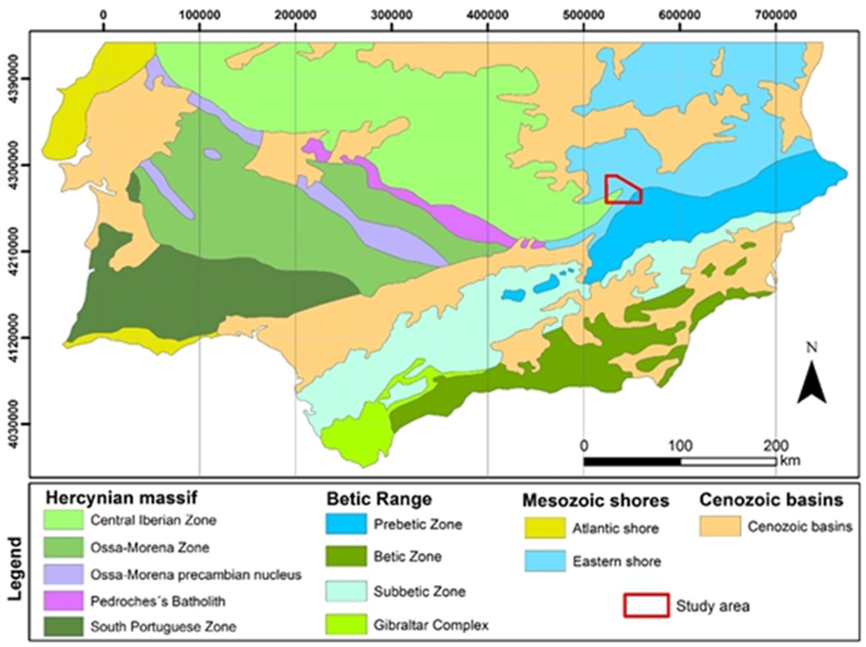
Figure 5 it can be seen with the naked eye that the spatial patterns of soil quality derived from the 12 methods used are similar. The parent material played an important role in the spatial distribution of soil quality. A similar pattern can easily be seen when looking at both maps: the soil quality map and the geological one.
The quality of the soil in the study area is preferably moderate (Grade III) -green areas-, when using the TDS-L and MDS-L models. The maps made using the TDS-NL and MDS-NL models show a predominance of both “green areas” or “moderate quality” (Grade III) and “light blue areas” or “high quality” (Grade IV). Only a small percentage of the surface of the studied area, in all the models, has a very high-quality grade (Grade IV) “dark blue areas” and the areas that have soils of very low quality (Grade I) “red areas” (although in some maps the surface occupied by low-quality soils is 0.00 hectares, there are actually one to five soil profiles that are considered within this grade).
In the spatial distribution map, grade III (Moderate) of the TDS-L-W and TDS-L-A indices are the ones with the highest representation (442 and 498 km
2, respectively). However, the same grade III, in the TDS-L-N index only occupies 287 km
2 (
Table 6). The studied region occupies a total area of 810 km
2, therefore, grade III, in each of the TDS-L-W and TDS-L-A indices, occupies 54.5 and 61.5%, respectively. However, the same grade III, in the TDS-L-N index, only occupies 35.4% of the total extension.
In the indices made with a nonlinear equation (TDS-NL-W and TDS-NL-A), grade IV (High) is the one with the greatest extension on the map (470 and 497 km2, respectively). However, the same grade IV, in the TDS-LN-N index only occupies 252 km2. Grade IV, in each of the TDS-L-W and TDS-L-A indices, occupies 58.0 and 61.3%, respectively. However, the same grade IV, in the TDS-L-N index only occupies 31.1% of the total extension.
In the MDS-LW and MDS-LA indices, grade III (Moderate) is again the one with the largest area on the map (392 and 398 km2; that is, 48.4 and 49.1% of the surface total, respectively). However, the same grade III, in the MDS-L-N index occupies a very high area (492 km2), 60.7% of the total area.
In the indices made with a nonlinear equation (MDS-NL-W and MDS-NL-A), grade III (Moderate) is the one with the greatest extension on the map (413 and 383 km2; that is, 51, 0 and 47.3% of the total area, respectively). However, the same grade III, in the MDS-LN-N index occupies a very high area (553 km2), 68.3% of the total area.
Summarizing, the surface percentages of the different degrees of soil quality obtained in the TDS and MDS models are similar with the use of the Weighted Additive (W) and Additive (A) methods; however, with the Nemoro (N) method the results are inferior (they are underestimated).
In general, the studied area is an important area for the agricultural production of rainfed cereals (preferably wheat and barley), due to its high soil fertility, aptitude for agriculture and potential productivity. If we make a geographical distribution of the quality of the soil types in the studied region, three zones can be distinguished: (1) zone of very low–low quality (red and yellow colors), which corresponds to Entisols developed on quartzites, slates and sandstones, located in the Sierra del Relumbrar, in the valleys on Triassic sandstones that surround the Sierra del Relumbrar and on dolomites in the Mesozoic Covert of the Iberian Massif; (2) of moderate quality (green zone), located in the central part of the map, which closely corresponds to the predominance of the Inceptisols and Alfisols developed over dolomites and maciños of the Sierra de Alcaraz and over deposits of the glacis surrounding Sierra del Relumbrar and (3) high–very high quality (light blue and dark blue colors), which closely corresponds to the predominance of Inceptisols, Alfisols, Mollisols and Vertisols’ developed deposits of glacis and clays and marls from the Mesozoic Covert. and the Sierra de Alcaraz.
Considering the expert opinion of agricultural technicians and farmers, the soils of this region are considered predominantly of moderate–high quality, especially for rain-fed cereal cultivation. Digital soil maps, which identify areas with different soil quality grades, can be used to facilitate better land management and avoid soil degradation processes.
3.4. Validation of Quality Indices
To compare the different indices, the precision of the classification for each quality grade was evaluated using the Kappa statistic and the correlation coefficients [
52,
57]. For Kappa analysis, a value was calculated to show the following levels of agreement [
61,
62]: (1) null: <0.05; (2) very low: 0.05–0.2; (3) low: 0.2–0.4; (4) moderate: 0.4–0.55; (5) good: 0.55–0.7; (6) very good: 0.7–0.85; (7) near perfect: 0.85–0.99; and (8) perfect: 1.
The evaluation of the agreement of the degrees of quality determined by the TDS and MDS indices and between linear scoring methods: that is, between the TDS-L-W and MDS-L-W and between TDS-L-A and MDS-L-A, in both cases the same Kappa value (0.45 (moderate)). The evaluation of the agreement between the quality grades determined by the TDS-L-N and MDS-L-N indices has resulted in a Kappa value of (0.42 (moderate)).
When comparing the agreement between the nonlinear scoring methods, the Kappa statistical values are as follows: between the TDS-NL-W and MDS-NL-W indices, a Kappa value of (0.38 (low)) has resulted. Between the TDS-NL-A and MDS-NL-A indices a Kappa value of (0.40 (between low and moderate)) has resulted. Finally, between the TDS-NL-N and MDS-NL-N indices, a Kappa value of (0.29 (low)) has resulted.
According to the Kappa analysis, the lowest levels of agreement are presented in the indices calculated using a nonlinear score and the Nemoro method.
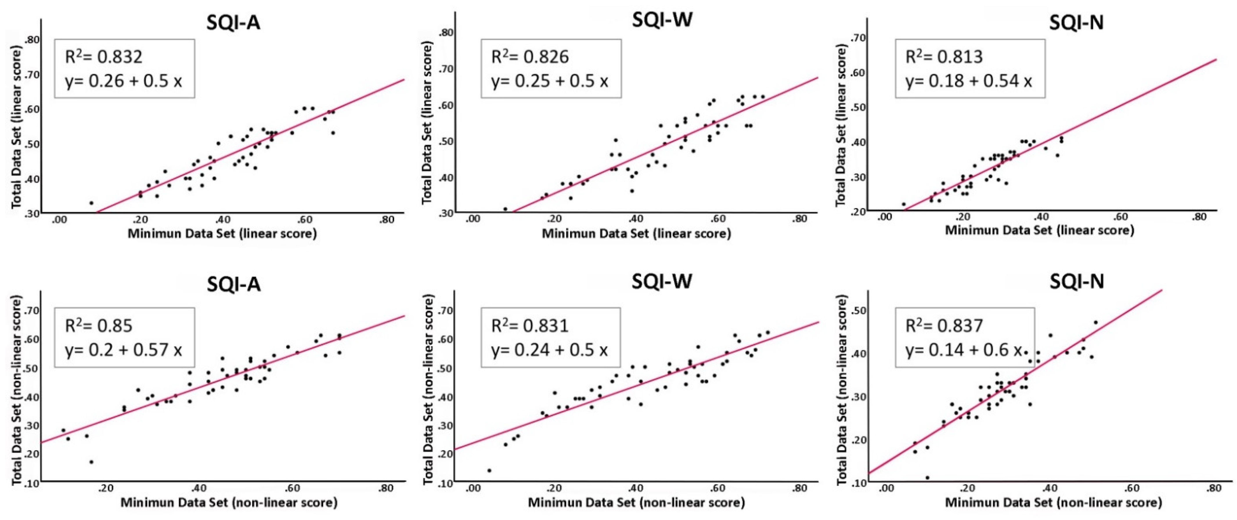
When performing the validation of the quality indices, using the TDS and MDS approaches (
Figure 6) through the use of correlation coefficients, they have been highly correlated with each other (all R values are very high, between 0.81 and 0.85). The highest coefficient (R = 0.85) resulted when using the TDS and MDS-NL-A (additive and nonlinear scoring) models. When using the TDS and MDS-L-A models, and TDS and MDS-L-W (Additive and Additive weighted and linear scoring) are used, in both cases a coefficient very similar to the previous one (R = 0.83) results.
The lowest coefficient (R = 0.81) results from the use of the TDS and MDS-L-N models (Nemoro and linear score).
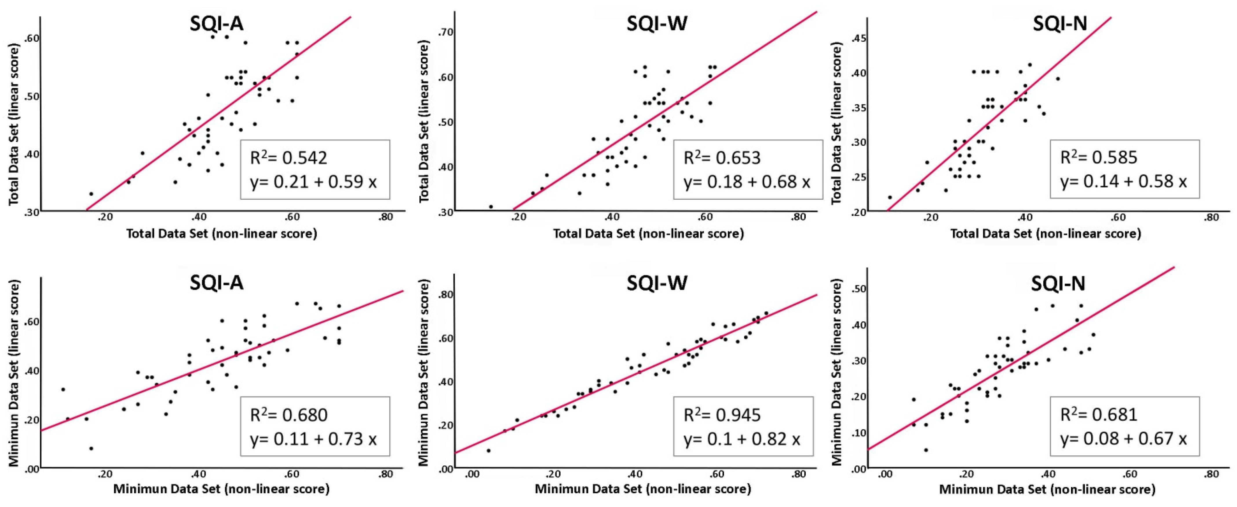
R values between 0.54 and 0.95 have been obtained by correlating the quality indices using linear and nonlinear scoring methods (
Figure 7). Of the six correlations made, five have values between 0.54 and 0.68.
The highest coefficient (R = 0.95) has resulted when using the MDS-L-W and MDS-NL-W models (weighted additive models and linear and nonlinear scores, respectively).
The results obtained, based on the Kappa statistics and the correlation coefficient, indicate that SQIW and SQIA models provide a better evaluation of soil quality than SQIN. The SQIW and SQIA models determine the quality of the soil using all the indicators and assigning higher weights to the indicators considered to be the most important in the evaluation. In contrast, the SQIN model uses the average value of all the indicators and the lowest scoring indicator, which gives it a higher weighted value. In other words, while the SQIW and SQIA independently assign the score for each indicator, the SQIN only gives preferential importance to the indicator with the lowest score.
By way of conclusion, it can be indicated that the indices that best reflect the state of soil quality are the SQITDS-L-W, SQITDS-L-A, SQITDS-NL-A and SQITDS-NL-W indices, as they are the most accurate indices and provide the most consistent results, since they consider all soil parameters. Normally, the more indicators the better the soil quality is represented, but it can happen that there is a high correlation between some of the selected properties of the soils, and this translates into a duplication of data and very laborious laboratory analysis. The evaluation method using the minimum data set avoids duplication of data and significantly reduces the labor and financial costs associated with sampling and analyzing data. As shown in the present study, the SQIMDS-L-W and SQIMDS-L-A methods provide an acceptable assessment of soil quality in large-scale studies.
Below, and as an example, the equations that define four of the quality indices that best represent the quality of soils are indicated.
As a result of applying the formula in Equation (7), the SQITDS-L-W soil quality index proposed in this work is represented in the Equation (9). The variables that make up the equation are ordered according on the weight or load value of the sixteen indicators:
If the formula in Equation (6) is applied, the SQITDS-L-A soil quality index that result can be seen in Equation (10). The variables of the equation are the sixteen scores of the indicators:
The SQIMDS-L-W soil quality index is represented by Equation (11). The variables that make up the equation are ordered according to the value of the load of the six indicators:
The SQIMDS-L-A soil quality index proposed in this work is given by Equation (12). The variables that make up the equation are the six indicator scores:
On average, the order of relative contribution of the selected indicators to the estimation of the SQI has been the following: water retention, water retention, the content of Calcium and Magnesium, the percentage of Clay, the Extractable Exchange Capacity, the content in Calcium Carbonate Equivalent, the Ph, etc. (see Equation (9)) This clearly reflected the influence of the weighting factors attributed through factor analysis.
The specific contribution of each MDS indicator to SQI shows that water retention had the highest contribution to SQI, followed by calcium content, equivalent calcium carbonate content, clay percentage, magnesium content and organic carbon content (see Equation (11)).
The validity of the method used can be confirmed with the opinion of agricultural experts in this region, who consider deep soils to be the best soils in this region (very high–high quality), which corresponds to Vertisols, Alfisols, Inceptisols and Mollisols, developed on clays, marls and deposits of glacis, the Mesozoic Covert and Sierra de Alcaraz. These are clayey soils (preferably smectite-type clays), with high organic matter content, high water retention, high CEC and COLE. The results obtained show that the consideration of the properties of the subsurface horizons of the soils and, specifically, the clay texture and water retention, are of great value for the evaluation of soil quality, considering that the climate in this region is semi-arid, and the soil moisture regime is xeric, so the soils remain in a moisture deficit for a large part of the year (between the months of May to October). The yield of rainfed crops will depend, mainly, on the moisture content stored in the subsurface horizons of the soil profile. Furthermore, the quality increases with the presence of a carbonate accumulation horizon and a pH close to neutrality, which is optimal for most crops.
According to agricultural experts, the properties that provide the highest quality to the soils of this region coincide with the indicators with the highest loads (high water retention, moderate percentage of clay, high CEC and COLE, neutral pH, moderate content of carbonates, etc., (see Equations (9) and (10)).
The soils with MODERATE quality closely correspond to the predominance of Inceptisols and Alfisols, developed on dolomites of the Sierra de Alcaraz and on deposits of the glacis that surround the Sierra del Relumbrar. Generally, with soils in which the loam–clay–sandy and clay–sandy textures predominate, in horizons A and B, respectively. In addition, they usually present clay content, water retention and a CEC with moderately high values. The pH values usually vary between 5 and 7.
The LOW quality soils correspond to thin soils (Entisols) developed on quartzites, slates and sandstones, located in the Sierra del Relumbrar, in the valleys on Triassic sandstones that surround the Sierra del Relumbrar and on dolomites in the Mesozoic Covert. of the Iberian Massif. These are soils of small thickness, formed by a single ochric epipedon, which rests on quartzites, slates, dolomites or sandstones. They are noncalcareous soils; the texture is usually loam–sandy or sandy–loam. The pH values vary between 4 and 6. They are very poor soils in nutritive elements for plants, with very low water retention; the degree of saturation is very close to 50% and the COLE has very low or insignificant values. These soils, traditionally, have been lent for land use dedicated to extensive livestock (grasslands).
3.5. Soil Quality Assessment Based on Land Use and the Different Parent Materials
The resulting values corresponding to the soil quality indices TDS-L-W and TDS-L-A of the three different types of land use (woodland, grassland and cropland) were 0.45, 0.45 and 0.52, respectively. The values of the TDS-NL-W and TDS-NL-A indices were 0.41, 0.44 and 0.50, respectively. The values of the indices calculated by the Nemoro method (TDS-L-N and TDS-NL-N) were 0.29, 0.30 and 0.35, respectively.
In summary, the TDS indices calculated using a linear and nonlinear equation and with the additive and weighted additive methods give higher values than the same indices, but calculated by the Nemoro method.
Similar results were obtained with the MDS indices calculated by means of a linear and nonlinear equation; with the additive and weighted additive methods they gave higher values (between 0.35 and 0.54) than the same indices, but calculated by the Nemoro method (between 0.24 and 0.34).
The mean soil quality values under crops were all significantly higher than those of the other land use. Due to the higher values of F and
p (
Figure 8), the values of the indices calculated with a linear equation were more sensitive than those calculated with a nonlinear equation.
The mean values for the twelve quality indices used were significantly higher for farmland than for grassland and forest soils. This fact suggests that there is a correlation (highly significant (p < 0.01 **) or probably significant (p < 0.05 *)) between the quality index and the land uses. The mean values of soil quality under forest use have been found to be equal to or slightly lower than that of grassland use.
Traditionally, the farmers of this region in this region have selected soils with the best edaphic properties for their agricultural use, and although, over time, conventional agriculture causes the degradation of some soil properties, agricultural soils and anthropogenic soils have maintained higher-quality levels compared to natural soils. In contrast, soils located in areas with a steep slope or shallow soils, with abundant rocky or stony, sandy texture, with low CEC, etc., are those that have been used solely and exclusively for grassland and/or forest use (holm oak cleared up).
In addition, in
Figure 8 it can be seen that the lowest average values of the quality indices are those obtained by the Nemoro method, both using linear and nonlinear scoring.
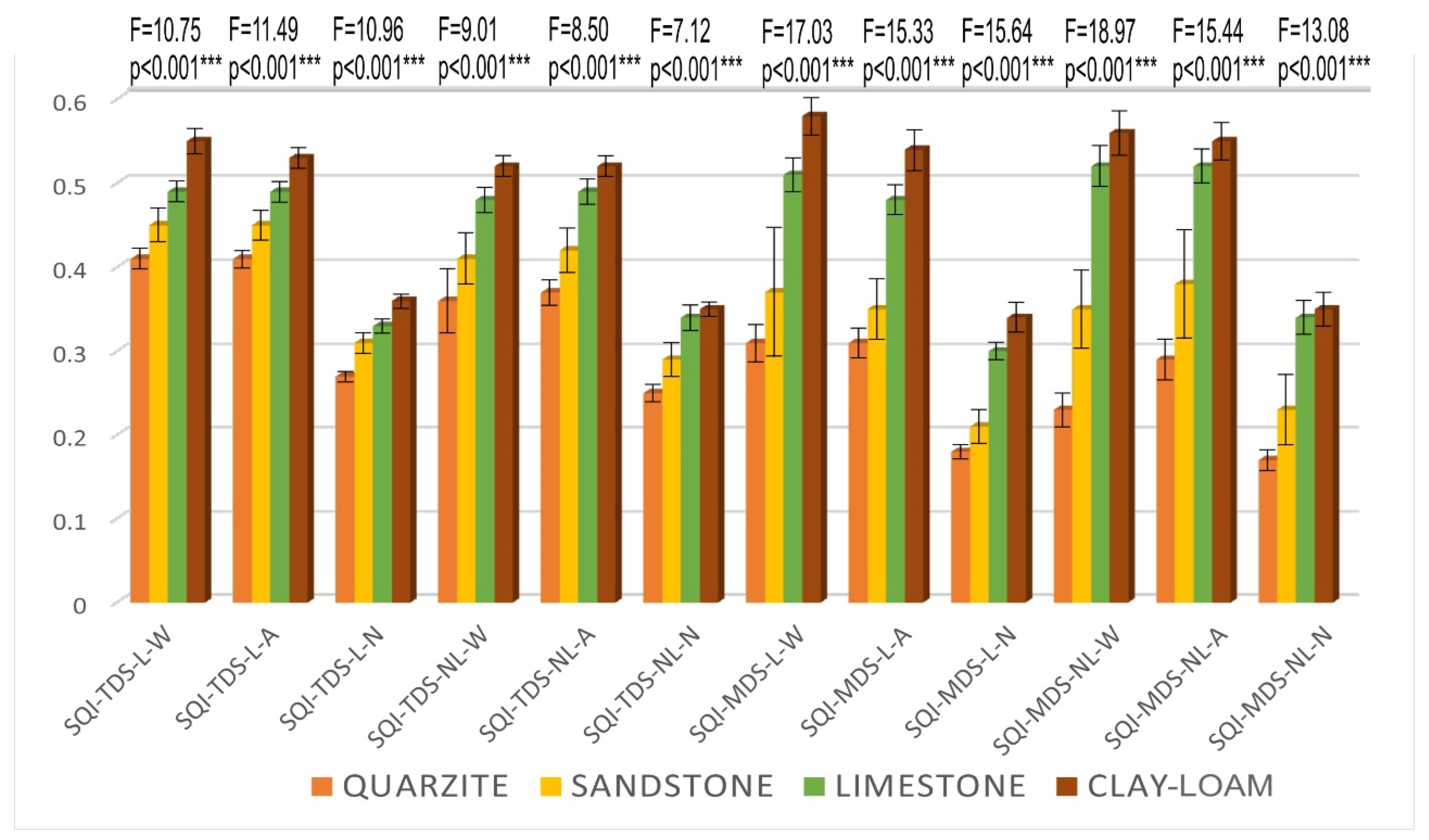
The resulting values corresponding to the quality indices TDS-LW and TDS-LA, of the four different types of source rocks of the soils (quartzite, sandstone, limestone and clay–loam) were 0.41, 0.45, 0.49 and 0.55, respectively. The values of the TDS-NL-W and TDS-NL-A indices were 0.36, 0.41, 0.48 and 0.52, respectively. The values of the indices calculated by the Nemoro method (TDS-L-N and TDS-NL-N) were 0.25, 0.29, 0.33 and 0.36, respectively.
Similar results were obtained with the MDS indices calculated by means of a linear and nonlinear equation; with the additive and weighted additive methods they gave higher values (between 0.23 and 0.58) than the same indices, but calculated by the Nemoro method (between 0.17 and 0.35).
The behavior of the soil quality indices in relation to the bedrock has been studied (
Figure 9); the mean values for the twelve quality indices used were significantly higher for soils formed on clays and/or loams, while soils formed on quartzites and/or blackboards presented the lowest SQI. The soils developed on limestones and/or dolomites presented a quality index that we could consider as moderate–high and moderate–low quality values were obtained on soils formed on sandstones. There is a highly significant correlation (
p < 0.001 ***) between all the quality indices and the parent rocks of the soils.
Again, it can be seen in
Figure 9 that the lowest average values of the quality indices are those obtained by the Nemoro method. In this sense, it can be observed in
Figure 8 and
Figure 9 that the highest values of the quality index are those obtained through linear and nonlinear equations.
The quality indices obtained by the MDS method evaluate the soils of the studied region through a selection of only six indicators, which represent the highest loads obtained through factor analysis (FA). Well, the order of relative contribution of these indicators to the estimation of the soil quality index is as follows: 22.8% for water retention, 22% for extractable Ca, 21.5% for CaCO3 equivalent, 21.2% for the clay content, 9.8% for the extractable Mg and 2.7% for the OC stock.
The score values of the water retention indicator at field capacity (GWC
1500kPa) varied from 0.41, 0.50 and 0.58 (linear) and 0.36, 0.45 and 0.52 (nonlinear) for grasslands, forest soils and farmland, respectively (
Figure 10A,B). These indicators score values (GWC
1500kPa), both linear and nonlinear, were highly significant (
p < 0.01).
A similar pattern was observed with the indicator score values (Clay), since the highest values are those obtained using a linear equation and correspond to croplands. On the contrary, the lowest correspond to grasslands
The score values of the indicators (CaCO3) and (Ca) have a totally different pattern from the previously studied indicators, since the highest values are those obtained using a nonlinear equation corresponding to croplands and the lowest values to forest soils. The score values of the indicators (OC Stock) and (Mg) also present as higher values those obtained using a nonlinear equation, but the highest values usually correspond to forest soils and values of pastures and farmland. They are very similar and even the same. These score values of the indicators (OC Stock) and (Mg), both linear and nonlinear, were significantly lower (p < 0.05).
The score values of the water retention indicator at field capacity (GWC
1500kPa) varied from 0.39, 0.42, 0.50 and 0.69 (linear) and 0.33, 0.36, 0.45 and 0.63 (nonlinear) for soils developed on sandstones, quartzites, limestone–dolomites and clays–marls, respectively (
Figure 10C,D). These indicators score values (GWC
1500kPa), both linear and nonlinear, were highly significant (
p < 0.001).
A similar pattern has been observed with the indicator score values (Clay), since the highest values (0.61, 0.66, 0.71 and 0.82) are obtained using a linear equation. Additionally, these higher values correspond to the soils developed on clay–loams and the lowest to those formed on sandstones.
The linear score values of the indicator (OC Stock) indicate that the soils with the highest content of organic matter are the soils developed on clay–loams and those with the least content are those formed from sandstones. On the contrary, the nonlinear score values offer us a different pattern, since the soils with the highest content of organic matter are the soils developed on sandstones and those with the least content are those formed from clay–marl and limestone–dolomites.
The score values of the indicators (CaCO3) varied from 0.00, 0.17, 0.32 and 0.39 (linear) and 0.00, 0.30, 0.55 and 0.58 (nonlinear), for soils developed on quartzites, sandstones, clays–marl and limestone–dolomites, respectively.
A pattern similar to the previous one has been observed with the indicator score values (Ca).
The highest indicator scores values (Mg) have corresponded to soils developed on clay–loams and the lowest values to those formed from sandstones.
Figure 11A shows the order of specific contribution of the six selected indicators to the estimation of the soil quality index (expressed as averages), according to the MDS method, for different land uses, using linear scoring functions. Between 60 and 70, 60% of the contribution of the indicators to the quality of forest soils and croplands is constituted, in decreasing order by (Clay), (GWC
1500kPa) and (Ca); in soils under grassland, the highest contribution (80%) is constituted by (Clay), (OC Stock), (GWC
1500kPa) and (Ca). The indicators (Clay), (GWC
1500kPa) and (Ca) can be considered as having the greatest influence on soil quality. In contrast, (Mg) and (CaCO
3) are the least influential.
However, using non-linear scoring functions (
Figure 11B), 80% of the contribution of the indicators to the quality of forest soils is made up, in decreasing order, by (OC Stock) (Mg), (GWC
1500kPa) and (Clay); in grassland soils the largest contribution (70%) is made by (OC Stock), (Clay), (Ca) and (GWC
1500kPa) and in cropland by (Ca), (CaCO
3), (OC Stock) and (GWC
1500kPa). In this case, in the non-linear scoring functions, the indicators with the highest influence on soil quality are (OC Stock), (Ca), (GWC
1500kPa) and (Clay) and the indicator with the lowest contribution to soil quality is (Mg).
Figure 11C shows the order of specific contribution of the selected indicators (expressed in averages) to the estimation of the soil quality index, for soils developed on different mother rocks, using linear scoring functions. Eighty percent of the contribution of the indicators to the quality of the soils developed on quartzites is constituted by (Clay), (GWC
1500kPa) and (OC Stock), in soils on sandstones and limestone–dolomites and clays-marls by (Clay), (Ca), (GWC
1500kPa) and (OC Stock). (Clay), (GWC1500 kPa), (Ca) and (OC Stock) can be considered as the indicators with the greatest influence on soil quality, and (Mg) and (CaCO
3) as those with the least contribution.
However, by using nonlinear scoring functions (
Figure 11D), 90% of the contribution of the indicators to the quality of the soils developed on quartzites is constituted by (OC Stock), (Clay), (GWC
1500kPa) and (Mg); in soils on sandstones the greatest contribution is formed by (OC Stock), (Ca), (Clay) and (GWC
1500kPa); in soils formed from limestone–dolomites by (Ca), (CaCO
3) and (OC Stock) and in soils on clay–loams by (Ca), (GWC
1500kPa), (CaCO
3) and (OC Stock). In this case, the indicators with the greatest influence on soil quality are (OC Stock), (Clay), (Ca), (GWC
1500kPa), and the indicator with the least contribution to soil quality is (Mg).
In summary, the indicators with the greatest influence on soil quality, obtained by the MDS method, for different land uses and those developed on different rocks, using linear scoring functions, are the following: (Clay), (GWC1500kPa) and (Ca). These data, in turn, coincide with the opinion of the agricultural experts of this region (who affirm that the best soils in this region are deep soils, with a clayey texture, with high water retention and a pH close to neutrality). However, the indicators with the greatest influence on soil quality, using nonlinear scoring functions, are: (OC Stock), (Clay), (Ca) and (GWC1500kPa). In other words, the most important indicator is the OC stock, which is not logical in the case of a region in which the soils have a very low average soil OC content (0.86%).


 ,
, 


