Article

Modeling of the 1783 Tsunami Event in Scilla Generated by Landslide

DICEAM Department, Mediterranea University of Reggio Calabria, Via Graziella loc. Feo di Vito, 89122 Reggio Calabria, Italy
*
Author to whom correspondence should be addressed.
Land 2022, 11(1), 69; https://doi.org/10.3390/land11010069
Submission received: 15 November 2021 / Revised: 24 December 2021 / Accepted: 28 December 2021 / Published: 3 January 2022

Abstract

:
In 1783, an event that has gone down in history as the great seismic crisis in Calabria began, during which two major earthquakes occurred, affecting the Calabrian ridge from the Strait to the north. Between 6 and 7 February in Scilla a tsunami occurred that caused the greatest number of victims in Italy: 1500 people. The mechanism that triggered the tsunami was the detachment of a ridge of rock due to a violent earthquake that affected the area; this detachment caused a subaerial landslide which, by sliding, then deposited the rock on the seabed a few kilometers from the coast, immediately generating the tsunami event. The objective of this study is to perform numerical simulations for tsunami events that occurred in history and use models that perform the propagation of a tsunami, using the best possible bathymetric and topographic data and the historical data to compare the validity of the results. In this way, one can obtain the validation of a model that can be used to simulate possible events of this magnitude on the Calabrian coasts and therefore be able to develop a reliable early warning tsunami system; it also has the advantage of perfectly combining computational burdens and the validity of results.

1. Introduction

Tsunami refers to an anomalous and imposing wave motion of the sea, originating from a very violent underwater earthquake, often of magnitude > 8.0 Richter, or from other events that involve a sudden displacement of a large body of water, such as a landslide or an underwater volcanic eruption [1,2]. On the Italian coast, several tsunamis have been documented in the last thousand years, only some of which have been destructive. The most important tsunami events are documented in the catalog of Italian tsunamis developed by Tinti et al. [3]. It describes how the coastal areas of eastern Sicily, Calabria, Puglia and the Aeolian archipelago, and those of the Ligurian, Tyrrhenian and Adriatic coasts, were affected by the tsunami. The most important tsunami event was that of 28 December 1908 [4,5]; it followed the earthquake in the Strait of Messina. During the event, the coasts of eastern Sicily and Calabria were hit by high waves that caused the deaths of hundreds of victims near the beach. The maximum run-up (maximum altitude reached by the water with respect to sea level) measured on the Calabrian coast was 13 m. The tsunamis of 1627 in Puglia, of 1783 in southern Calabria and of 1693 in eastern Sicily are also important to mention. The first tsunami of the last century occurred in Stromboli, in the Aeolian Islands, on 30 December 2002, causing a lot of damage to buildings along the coasts of the island. The study and the simulation of tsunami events that occurred in the Mediterranean Sea are fundamental because they can be used as a benchmark to test numerical models and to be able to estimate the hazards and risks optimally. One of the most important cases in the Strait of Messina was the 6 February 1783 landslide-induced tsunami in Scilla. During the “1783 Terremoto delle Calabrie” earthquake, there were five main shocks between M 5.8 and M 7.3; between 5 February and 28 March 1783, the southern part of Calabria was violently hit. A large number of shocks, already high because of the earthquake, caused certain phenomena, such as landslides; these are documented in historical sources [6]. The most important landslide occurred immediately after midnight in the south of Scilla, approximately 30 min after the 6 February earthquake and, flowing into the sea, triggered a tsunami with a high of 16 m; during this event, more than 1500 people died along the Marina Grande beach [7,8,9,10].
Zaniboni et al. [11] simulated the generation and propagation of the tsunami using the finite difference code UBO-TSUFD (Tinti and Tonini [12]), which solves frictionless nonlinear shallow-water equations with a staggered-grid technique and dynamic boundary conditions at the coastal flooding computations. Zaniboni et al. [13] extended the study to the area of Capo Peloro and Punta Faro in Sicily by using the same numerical models both for landslide and tsunami simulation of the previous investigation.
The paper analyzes the case study of the 1783 Scilla tsunami event. The topo-bathymetry and the movement of the landslide generated by the earthquake are modeled with the MATLAB and QGIS software packages. In this study, the numerical depth-integrated model developed by Bellotti [14,15,16] was used; in this model, the propagation of small-amplitude transient waves is developed using a mild-slope equation. The Fourier Transform is used in the model to convert the time-dependent hyperbolic equation into a set of elliptic equations in the frequency domain. This application is presented to show the importance of applying this method to real events; for good risk management of tsunamis, it is also necessary to reduce anthropization in coastal areas and a project to reduce coastal erosion on the Calabrian coasts. Indeed, the study of these two factors greatly influences the effects of tsunami inundation on the coasts [17,18,19,20,21,22].

2. Modeling Landslide and Tsunami

2.1. The Scilla 1783 Case

The destructive earthquakes of February–March 1783 destroyed all of central-southern Calabria and also caused damage in the Strait area and in the Messina area. There were five strong earthquakes in a short period of time, between 5 February and 28 March 1783, and many smaller events (Figure 1).
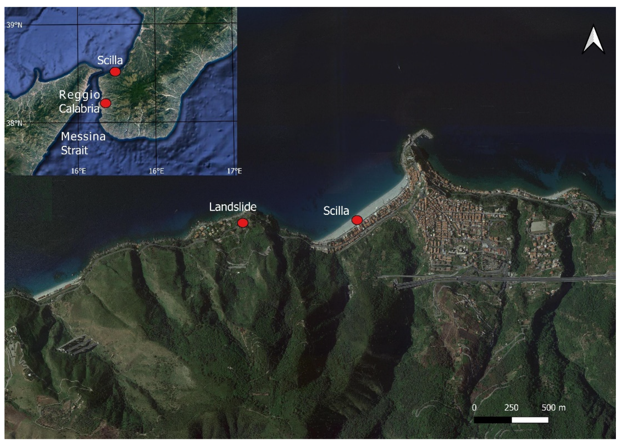
After the earthquake of 6 February 1783, there was a catastrophic tsunami in Scilla. Scilla is a small village near Reggio Calabria, one of the most graceful and characteristic in Italy, which stands on a high rocky spur overlooking the sea in front of the Messina Strait. The tsunami was not triggered directly by the shock but without doubt by a big landslide caused by the earthquake, described by historical sources. The location of the event is shown in Figure 2.
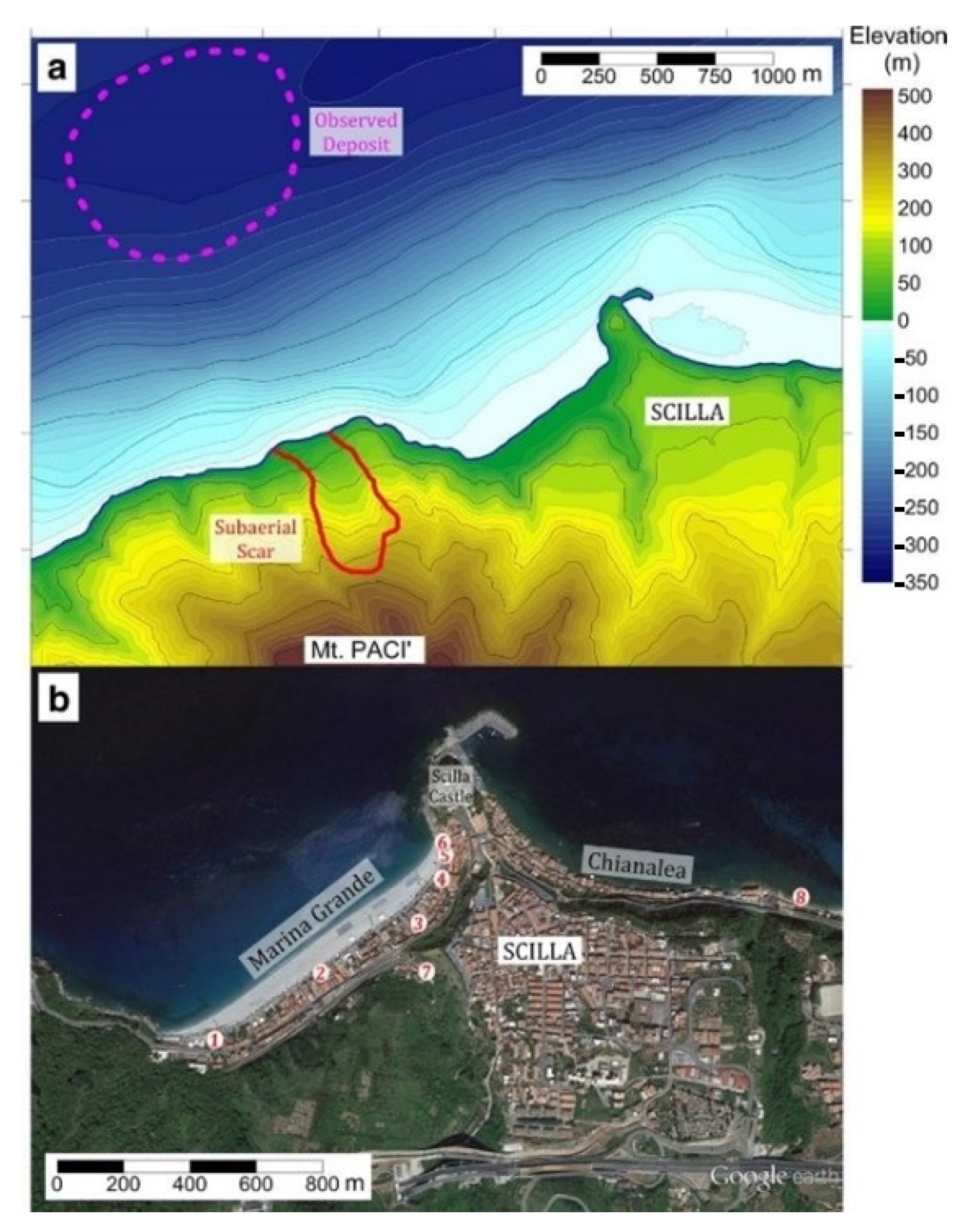
Many coeval and historical reports and studies described the events in detail [23] (Figure 3a). From these studies, it is possible to reconstruct some features of the tsunami.
The shore was hit by three main waves, with heights between 6 and 9 m (see Figure 3b for location). The flood in the land reached about 100 m, with a pick of 200 m near the Livorno stream, in the center of Marina Grande (point 7 in Figure 3b). The tsunami hit the outer walls of the Scilla Castle and the village of Chianalea (point 8, Figure 3b) on the other side of the Scilla promontory, where the waves reached 3–4 m high.
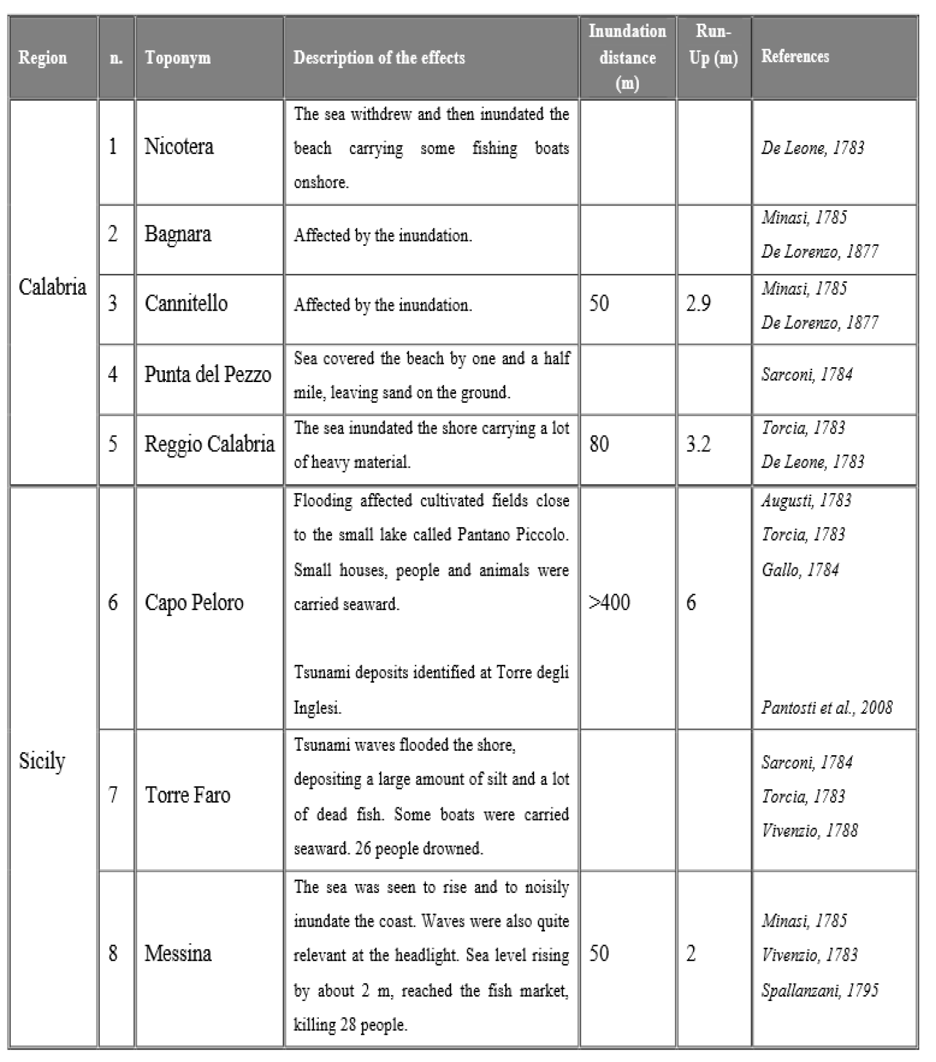
A large coastal part of Tyrrhenian Calabria, approximately 40 km long, was affected by the tsunami along with the coasts of Sicily and the harbor of Messina on the other side of the Messina Straits [24,25,26]. Taking into account the historical reconstruction of the earthquake, landslide and tsunami time sequence, the evidence of a landslide source for the tsunami can be demonstrated. Indeed, the historical evidence leads us to deduce that the landslide was triggered approximately 30 min after the earthquake and that the tsunami arrived in correspondence to Marina Grande beach about 30–60 s after the fall of the landslide; both the area near Scilla affected by the tsunami and the consequent wave height distribution support the hypothesis that the landslide was the origin of the tsunami. Maximum run-up heights of between 6 to 9 m, according to Sarconi, and up to 16 m, according to Minasi, were recorded along the Marina Grande beach, but also in the Calabrian coasts between Nicotera and Reggio Calabria, as well as along the Sicilian coast, many towns and villages, such as Cannitello, Bagnara Calabra, Punta del Faro and Messina, were hit by the wave. As shown in Figure 4, however, the wave run-up height and the inundation distance (based on historical documents) drastically decrease moving away from Scilla.
From Figure 5, one can observe that the effects of the tsunami were much less prevalent in the neighboring area than in Scilla. Remarkably, the waves were seen in Calabria from Nicotera (point 1, Figure 5), approximately 40 km north-east of Scilla, to Reggio Calabria (point 5, Figure 5), 20 km south-west. On the other side of the Messina Straits, the place closest to the source is the easternmost corner of Sicily, is Capo Peloro (point 6, Figure 5), next to the village of Torre Faro (point 7, Figure 5). Here, the tsunami was strong and disastrous. In addition to historical sources, the impact of high-energy tsunami waves in this area was confirmed by recent geological investigations carried out in a site called Torre degli Inglesi (Capo Peloro, point 6, Figure 5), approximately 40 m from the present shoreline, where a 15 cm thick sand deposit in a trench layer sequence was attributed to the 1783 event.

2.2. Depth Integrated Wave Model

The model is based on the hyperbolic wave equation; this equation has a source term that is the second derivative in time of the varying water depth, altered by the passage of the landslide. This same approach has been applied for the nonlinear shallow water equations [27], and in this case, in the forcing term of the continuity equation, there is a filter function in order to consider when the water depth is not much smaller than the landslide length. The continuity equation is:
η t + h · ( vh ) = h t 1 cos h ( k s h )
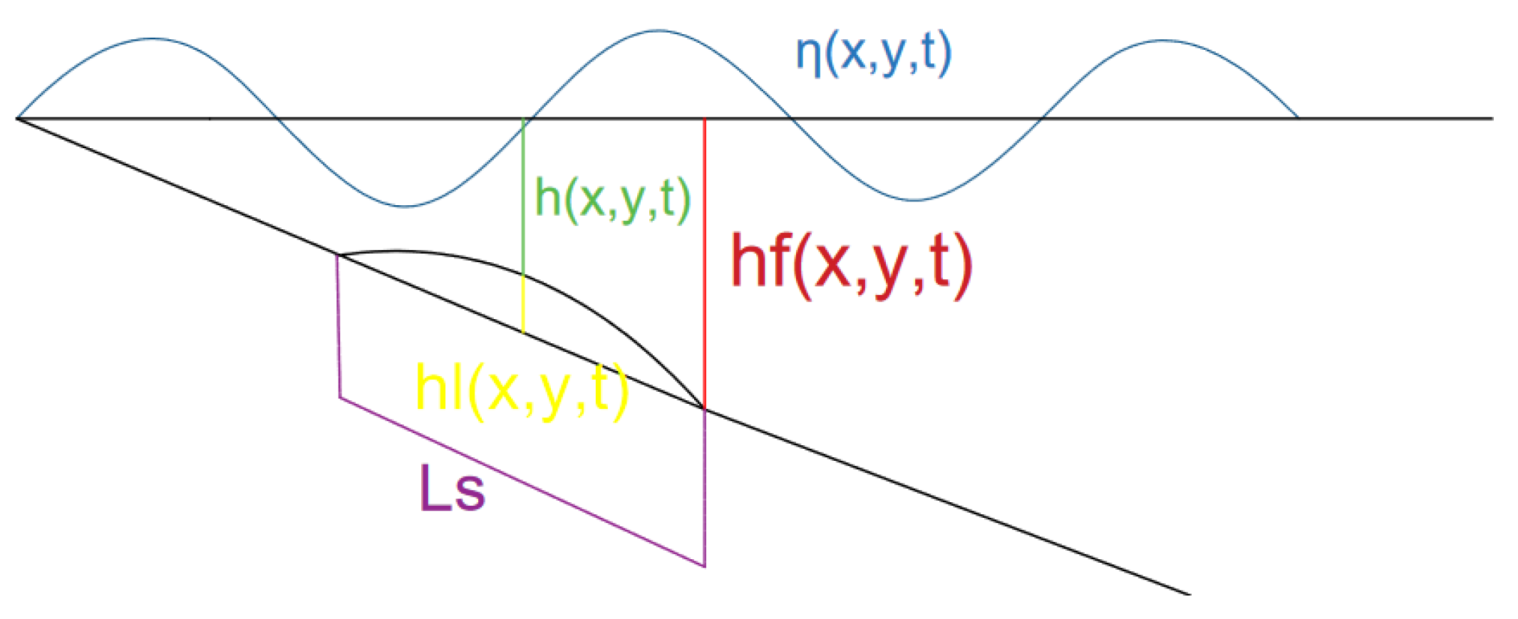
where η(x,y,t) is the free water surface, v(x,y,z,t) is the fluid particle velocity, h(x,y,t) = hf(x,y) − hl(x,y,t) is the water depth function defined as the fixed seafloor depth (hf) minus the thickness of the moving landslide (hl). ks is the landslide length parameter, equal to 2π/Ls, where Ls is the landslide length (Figure 6).
Cecioni and Bellotti [28] described and validated in more detail a method based on the depth-integrated mild slope equation (hereinafter MSE), which they reported in their previous paper [29]. In their work, they introduced the effects of the moving sea bottom by using a new function in order to simulate the waves generation. The new function that represents the source term, which is in the MSE, is similar to that of Tinti et al., in Equation (1), but in this case, the dependence of the filter function is based on the wavelength and not on the landslide length. Cecioni and Bellotti demonstrated that this technique is very accurate, taking into account a mild slope sea bottom, small amplitude waves and landslides, and it is essential when applying frequency-dispersive equations.

2.3. Methodology

Regarding the numerical simulation, the QGIS and Matlab software packages were used in the pre-processing phase for the interpretation and arrangement of the topographic and bathymetric data and the modeling of the landslide and its displacement; the COMSOL software was used to simulate the propagation of the tsunami from offshore to the shore, and finally, in the post-processing phase, MATLAB was used for the interpretation of the results. In order to deal with the numerical modeling of the phenomenon, there were several preparatory steps for the simulation that can be summarized in 11 points (Figure 7):
  • Acquisition of geographic data from IGM (Military Geographic Institute). The IGM (Military Geographic Institute) provided the bathymetry as 80 vector files with unstructured data. The original reference system was WGS 84/UTM zone 33N, so each file was first converted to a shapefile using QGIS while maintaining the same georeferencing.
  • Construction of the geographical domain by using QGIS;
  • Creation of a single file with all the georeferenced bathymetric data available and importation into MATLAB to be processed. A grid was created to interpolate the data, which were not structured, with Δx = Δy = 10 m, where Δx and Δy are the spatial nodes into which the grid is divided, the interpolation concerned the three coordinates x, y and z;
  • Extrapolation of a subdomain, the one corresponding to the passage of the landslide, to evaluate its displacement over time. The domain concerned had dimensions of X = 360 m axis parallel to the coast and Y = 1400 m approximately orthogonal axis to the coast and reached a depth of −300 m in which the landslide was deposited in its final position;
  • Evaluation of the geometric shape of the landslide; the simulation of the landslide over time by Mazzanti and Bozzano [30,31] was taken as a reference;
  • The bathymetric subdomain extracted, corresponding to the passage of the landslide, is reworked in MATLAB in order to create an ellipsoidal grid;
  • Estimation of the simulation of the displacement of the landslide at different time points;
  • Identification of the geographic domain to be included in COMSOL, where the characteristics of the model were then assigned;
  • Creation in MATLAB of an array that represents the position of the landslide in the spatial dimensions x and y at various time points. The result was, therefore, a set of matrices that represent the spatial position, and in the third dimension, there was spatial variation over time.
  • Insertion of boundary conditions and COMSOL mesh;
  • Wave propagation simulation in COMSOL software and extrapolation of the results.

2.4. Geographic Data and Domain

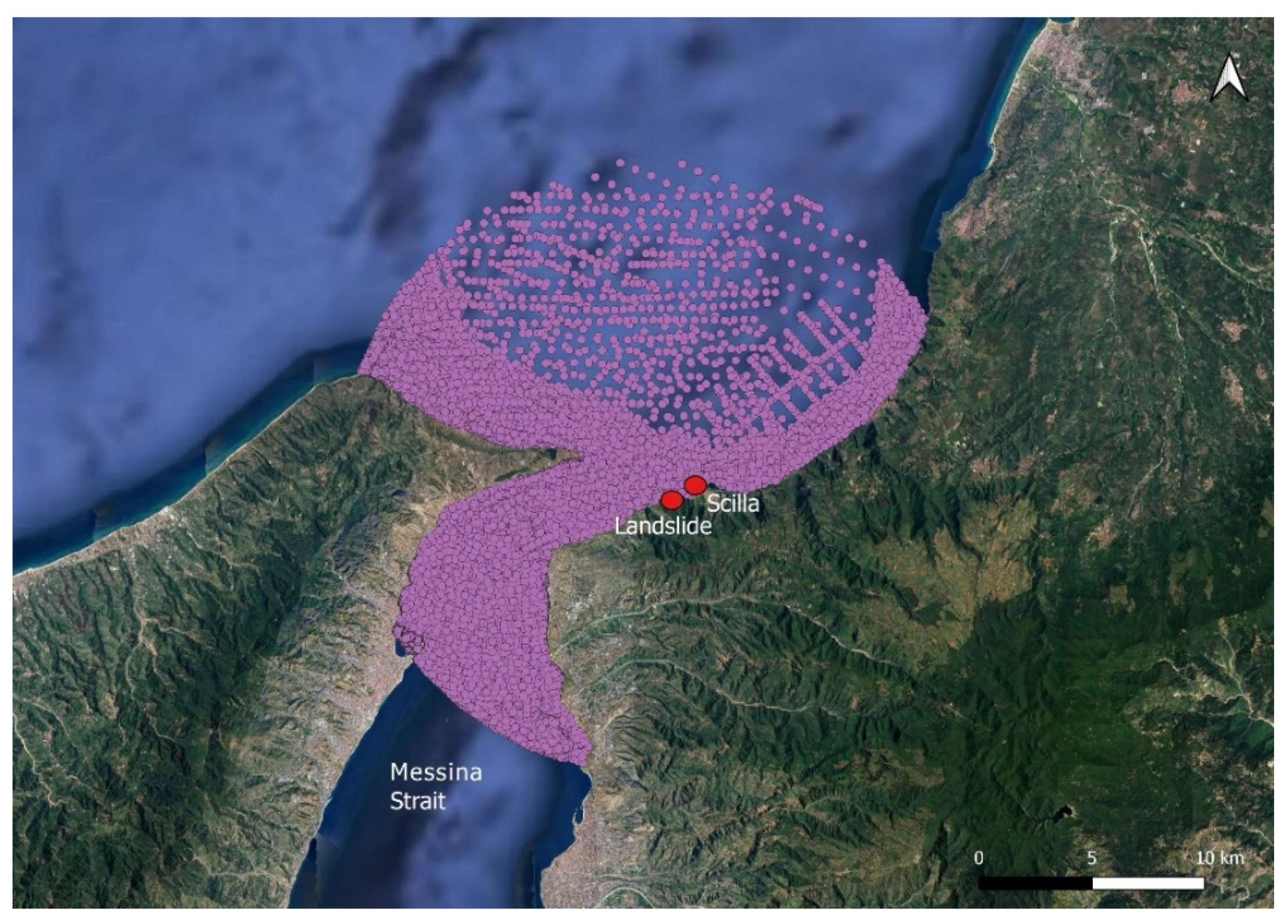
The model grid requires a depth matrix developed by interpolating bathymetric and topographic data of the resolution commensurate with that of the grid. Bathymetry and topography for the grid were interpolated for the most accurate sources available. The IGM (Military Geographic Institute) provided the bathymetry as 80 vector files with unstructured data. The original reference system was WGS 84/UTM zone 33N, so each file was first converted to a shapefile using QGIS while maintaining the same georeferencing (Figure 8).
Once a single file was created with all the georeferenced bathymetric data available, they were imported into MATLAB to be processed. A grid was created to interpolate the data, which are not structured, with Δx = Δy = 10 m. The interpolation concerned the three coordinates x, y and z.
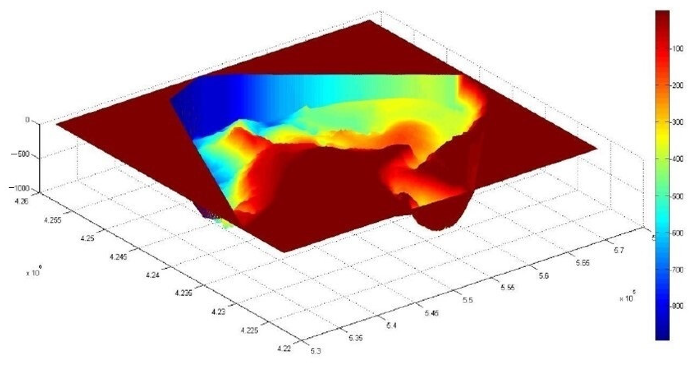
The meshgrid features are summarized in the following Table 1 and shown in Figure 9 and Figure 10:

2.5. Landslide Modeling

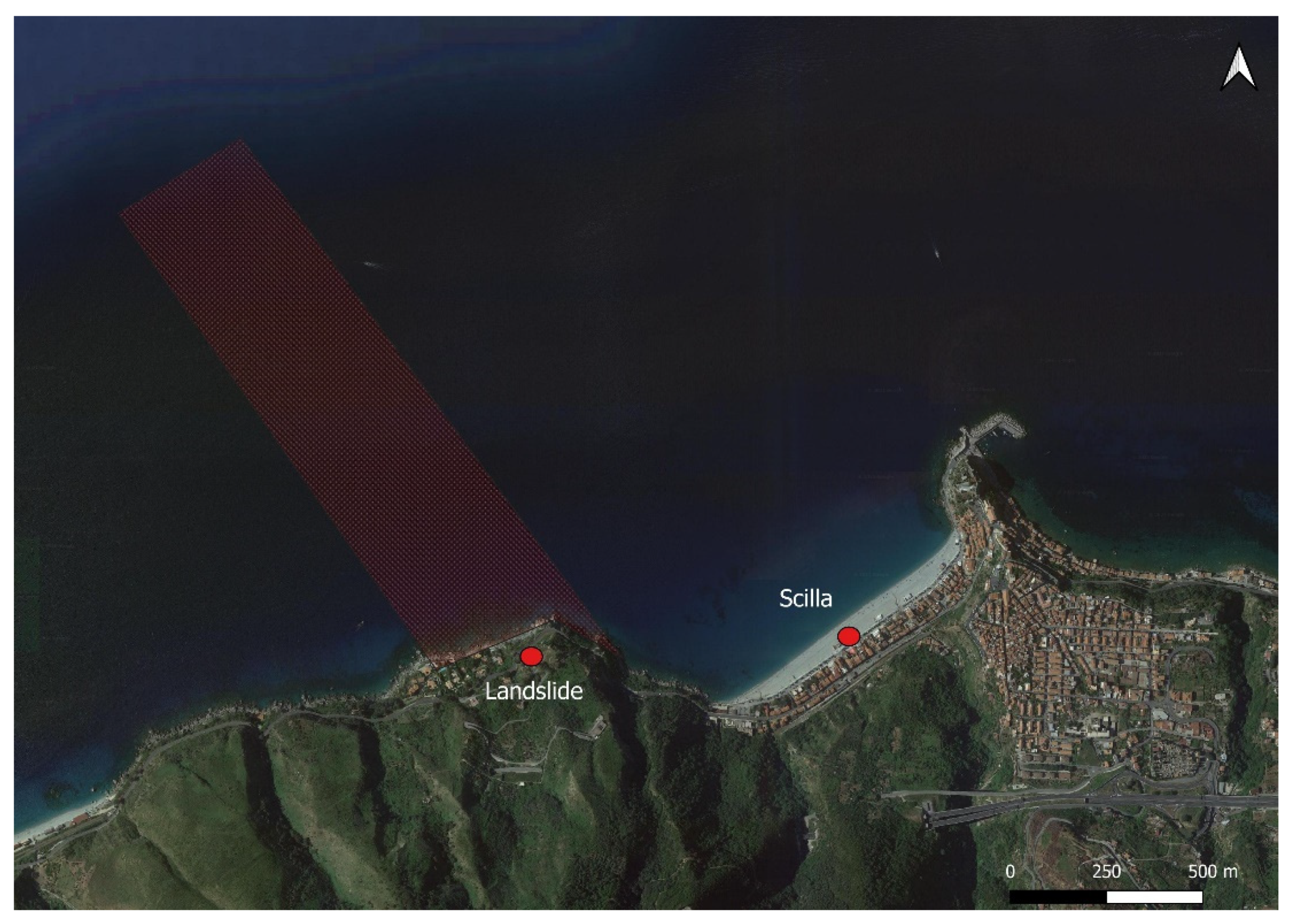
Once the domain was created, a subdomain was extrapolated, corresponding to the passage of the landslide, to evaluate its displacement over time. In Figure 11, the position of the subdomain is shown.
The domain concerned had the dimensions X = 360 m axis parallel to the coast and Y = 1400 m approximately orthogonal axis to the coast, and reached a depth of −300 m in which the landslide was deposited in its final position.
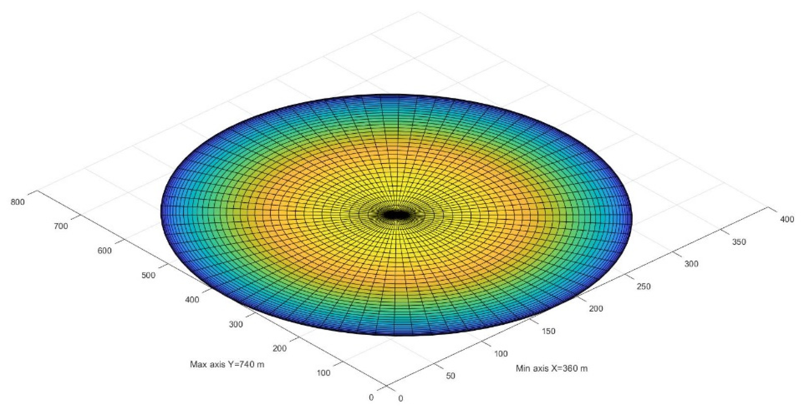
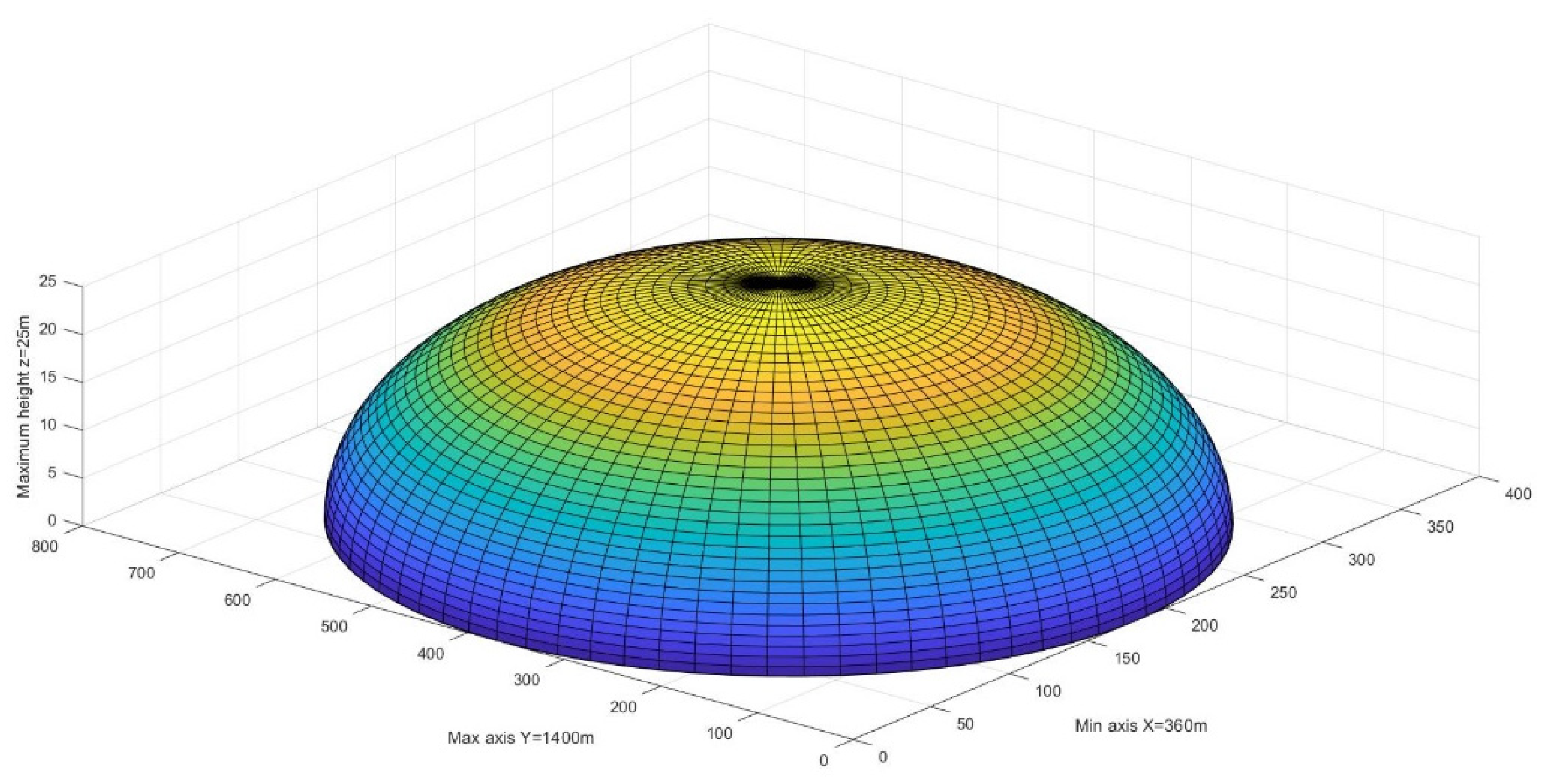
The first step was the evaluation of the geometric shape of the landslide. The simulation of the landslide over time in Mazzanti and Bozzano [31] was taken as a reference. Using that simulation as a starting point, the geometric quantities were taken for each simulated time point (length, width and height). Then an ellipsoidal profile was reconstructed on MATLAB by the average value of these quantities (Figure 12 and Figure 13). The landslide had a maximum height of 25 m, a length of 740 m and a width of 360 m.
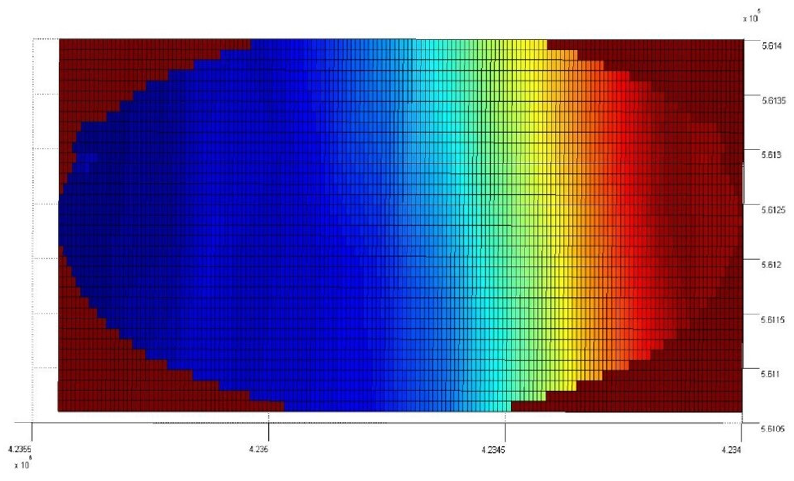
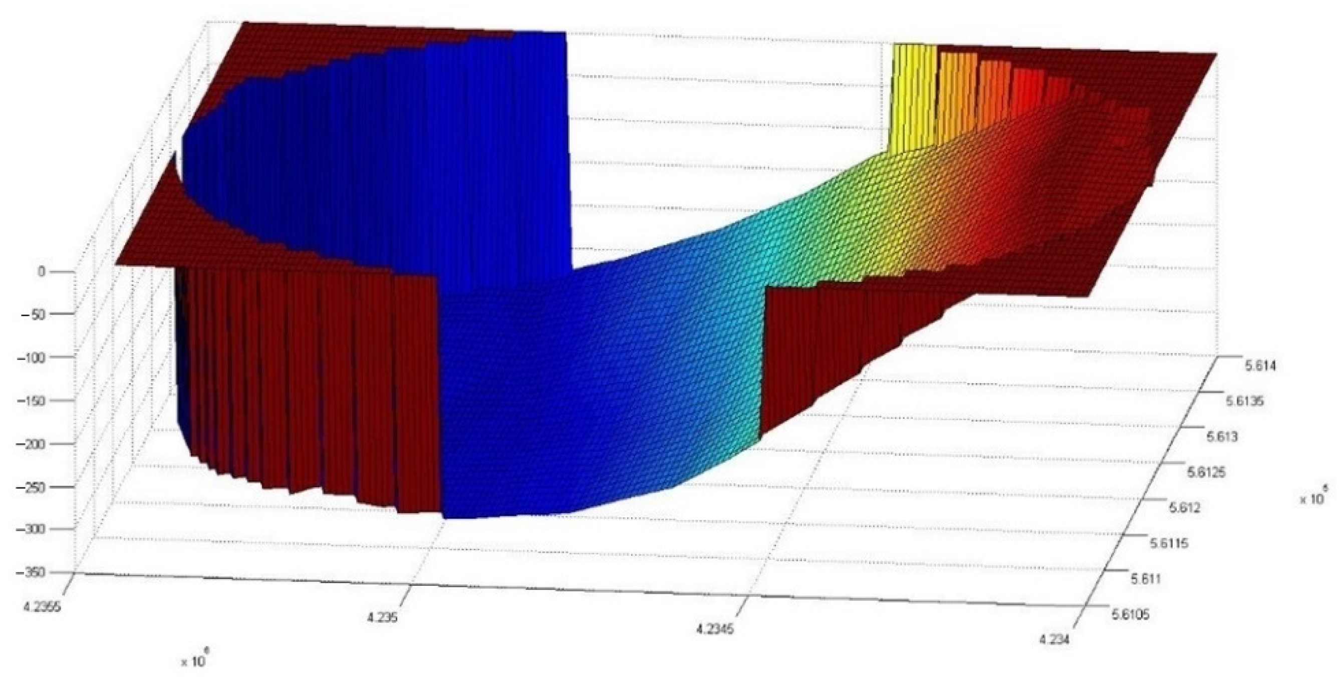
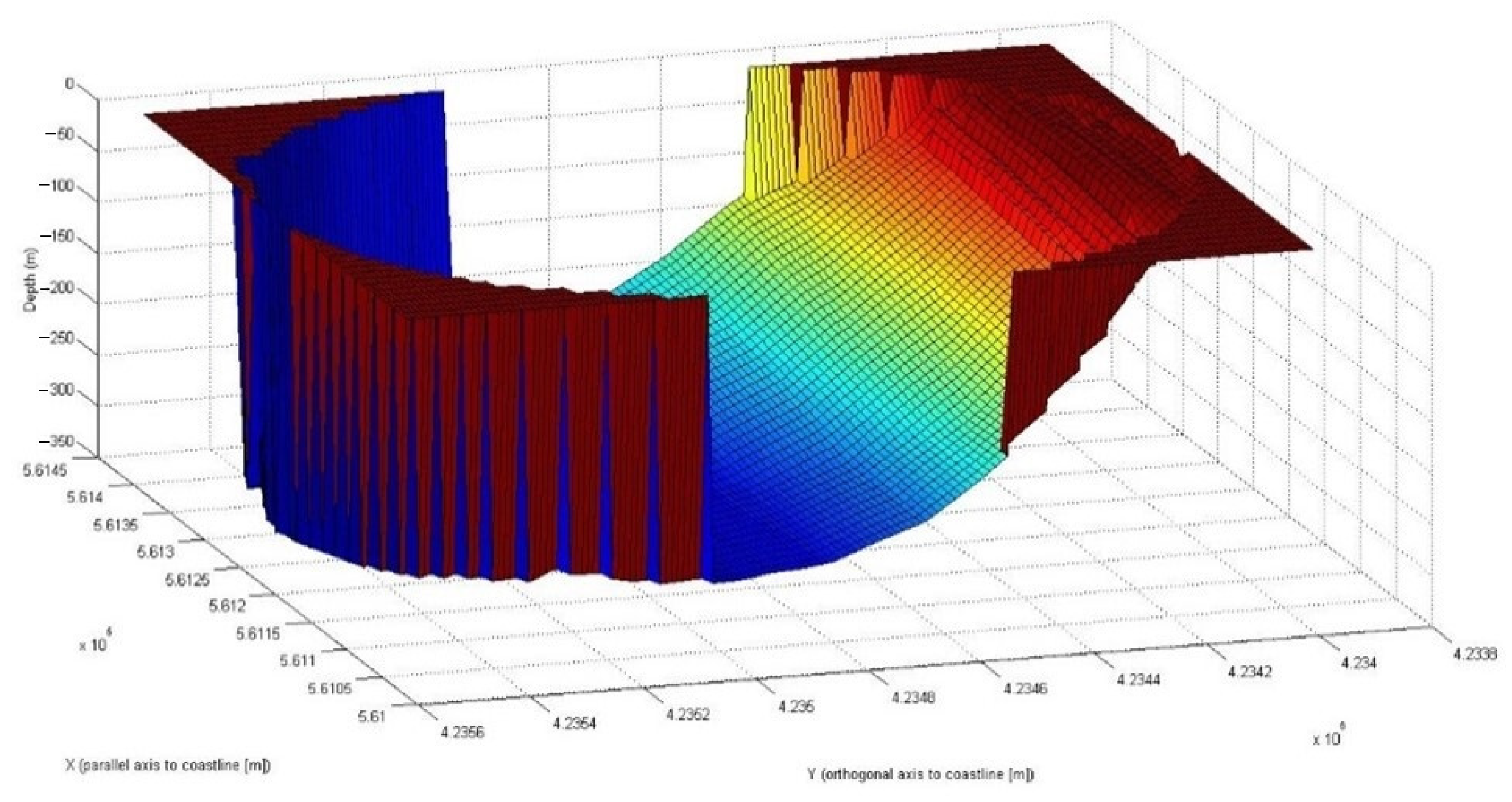
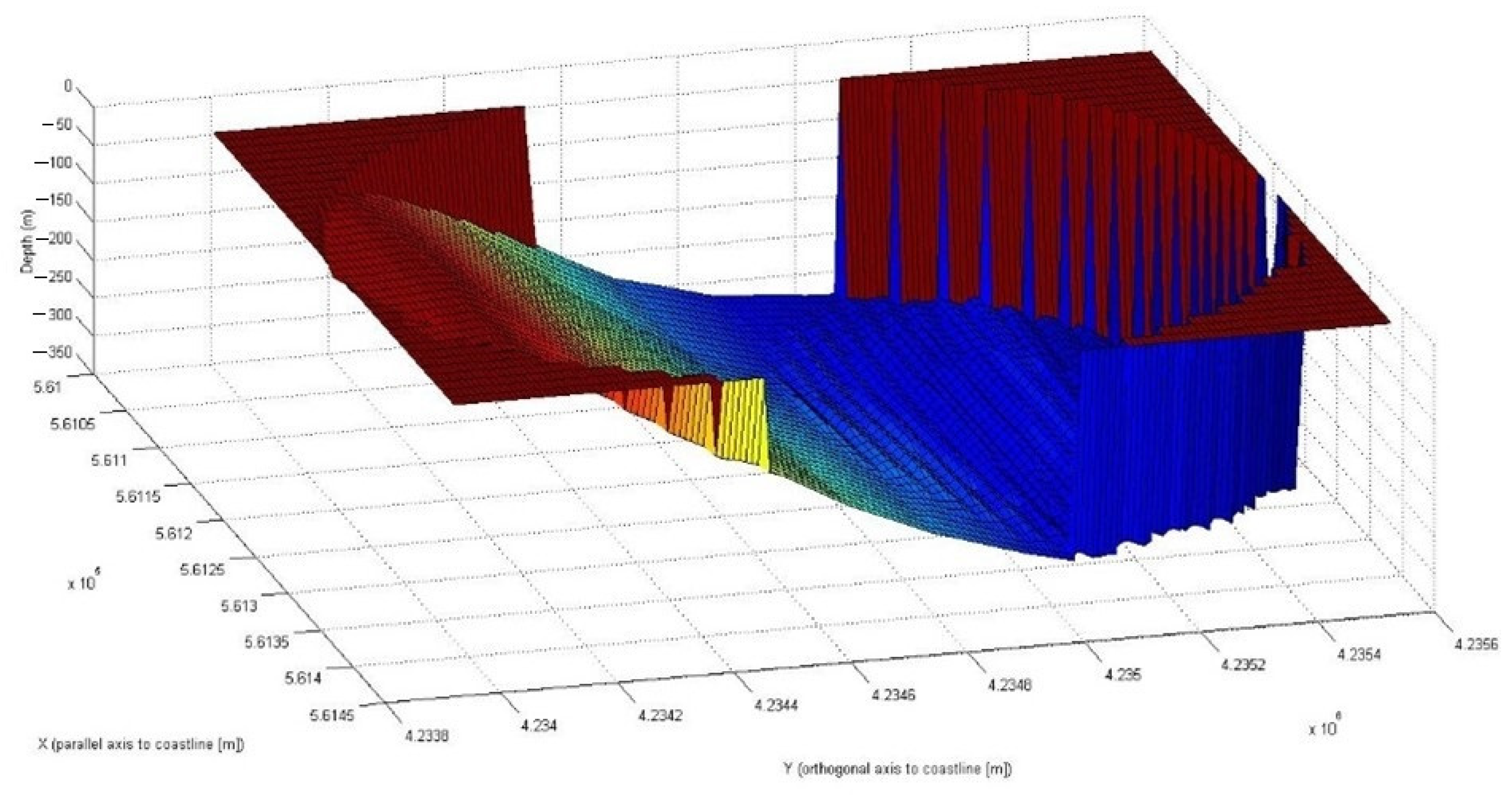
Since an ellipsoidal geometric shape of the landslide was hypothesized, the bathymetric subdomain extracted corresponding to the passage of the landslide was reworked in MATLAB in order to create an ellipsoidal grid (Figure 14 and Figure 15).
This made it possible to obtain the correspondence between the points of the bathymetric grid and those of the landslide, which is necessary for the subsequent calculation of the source term.
In order to work on the displacement, the domain on which the landslide moves was always modeled with Δx = Δy = 10 m.
The following Table 2 summarizes the geometric features of the bathymetric subdomain:
Once the domain had been created, the time and velocity of movement of the landslide were evaluated; to do this, reference was continuously made to the article by Mazzanti and Bozzano (2011). The authors simulated the 1783 Scilla landslide using a DTMM (Digital Terrain and Marine Model) with 20 m square cells, obtained by combining subaerial DTM (based on a 1:5000 topographic map) and high-resolution bathymetry collected by sonar multibeam surveys. A detached volume of 5.4 × 10⁶ m3 and a maximum run-out of 2.5 km from the upper scar were considered in the numerical back-analysis. Their simulation results show that the mass reaches the flat area in front of Scilla after about 40 s and the final run-out after 80 s; in the following 40 s (from 80 to 120 s), only a lateral spreading of the material is observed. A maximum landslide velocity of 45 m/s is reached about 15–20 s after the failure in the frontal part of the mass (in the submarine slope). Then, the moving mass maintains a velocity greater than 40 m/s until 30 s that decreases below 20 m/s after 60 s from the collapse. After 70–80 s, the mass moves at a rate lower than 10 m/s. Historical documents testify to an intense 30 s long noise coming from Monte Pacì before the arrival of the tsunami (Minasi, 1785). The following Table 3 and Table 4 summarizes the time features of the landslide displacement in its subaerial phase and its submerged phase:
The simulation of the displacement of the landslide at different time points takes place, therefore, by calculating the following quantity for each spatial point and at each time point:
h(x,y,t) = hf(x,y) − hl(x,y,t)

2.6. Fully Dispersion Model Derivation

We start from the linearized (small amplitude) water wave equations for an incompressible irrotational fluid on an uneven bottom, considering two-dimensional horizontal propagation:
2 Φ + Φ zz = 0   h ( x , y ) z 0
Φ t + g η = 0   z = 0
η t Φ z = 0   z = 0
Φ z + Φ · h = 0   z = h ( x , y )
where φ(x,y,z,t) is the velocity potential in the fluid, η(x,y,t) is the instantaneous elevation of the free surface, h(x,y) is the water depth and g is the gravity acceleration. All these variables are real and scalar.
To simplify the problem we assume that:
φ(x,y,x,t) = φ(x,y,t)f(z,h)
where φ(x,y,t) is the velocity potential at z = 0 and f(z) is a function that describes how the kinematic field varies along with the water depth. Please note that, although not clearly indicated here, the function f may depend on the frequency of the waves and the local water depth, as detailed later. Bellotti et al. (2008) followed the procedure described by Dingemans (1997), who used a variational principle to derive two evolution equations, valid for the mildly sloping bottom, for the free surface elevation η and the velocity potential φ at the undisturbed water level z = 0:
η t = G φ · ( F φ )
φt = −gη
F and G depend on the specific function f and are more conveniently evaluated later. They are defined as:
F = h 0 f 2 d z
G = h 0 ( f z ) 2 d z
Equations (7) and (8) are respectively equivalent to a mass and to a momentum conservation equations (it is easy to show that for very long waves, f does not vary over the water depth and that (7) and (8) reduce to the linearized version of the NSWE). The first of these can be modified in order to incorporate the effect of the movements of the bottom, such as those occurring during earthquakes and submerged landslides. Equation (7), therefore, can be heuristically rewritten as
η t = G φ · ( F φ ) h t
provided that the horizontal scale of the area where the bottom moves is much larger than the scale of the water depth.
By eliminating φ between Equations (7) and (11), a single second-order hyperbolic equation for η is obtained:
η tt g G η · ( g F η ) = h t t
Equation (12) is usually referred to as the ‘time-dependent mild-slope equation’ and allows the simulation in the time-domain of the wave propagation. However, F and G are to be calculated by assuming a dominant frequency of the wave spectrum, and the validity of the resulting equation is only for narrow frequency-spectra seas. Here a spectral approach is used to solve Equation (12), resulting in a model which is valid for a broad spectrum wave field similar to those typical of tsunamis. The Fourier Transform of Equation (12) is calculated with respect to the time t (remember that f, and consequently F and G, does not depend on the time) yielding:
ω 2 N · ( g F N ) + g G N = ω 2 H
where N(x,y,ω) is the Fourier Transform of η(x,y,t), H(x,y,ω) the Fourier transform of h(x,y,t) and ω the angular frequency. Note that N and H may be complex numbers. Now for each value of ω, the function f can be chosen as that resulting from the linear wave theory valid for harmonic waves propagating in constant depth, which, however, still holds in the case of the mildly sloping bottom, i.e.,:
f = cos h [ k ( h + z ) ] cos h ( kh )
where the wave number k is obtained by solving the frequency dispersion relationship
ω2 = gktanh(kh)
F and G can be calculated for any value of ω as (Dingemans, 1997):
F = cc g g
G = ω 2 k 2 cc g g
where c and cg are the phase and group celerity, respectively. Equations (16) and (17), when inserted into Equation (13), lead to the elliptic version of the mild-slope equation (Berkhoff, 1972)
· (   cc g N ) + ω 2 c g c N = ω 2 H
The right-hand side term of Equation (18) represents the generation of the tsunami waves due to bottom movements during earthquakes and submerged landslides. This term could be set to zero if a wave-maker condition is imposed at one boundary. Here, however, it is to be kept in mind that several (potentially infinite) values of ω are to be considered and therefore, many equations such as (18) need to be solved to obtain the final result in the frequency domain. Once the equations (18) are solved with the appropriate boundary conditions, the result in the time-domain can be obtained by taking the Inverse Fourier Transform of N(x,y,ω) to obtain η(x,y,t).

2.7. Numerical Simulation

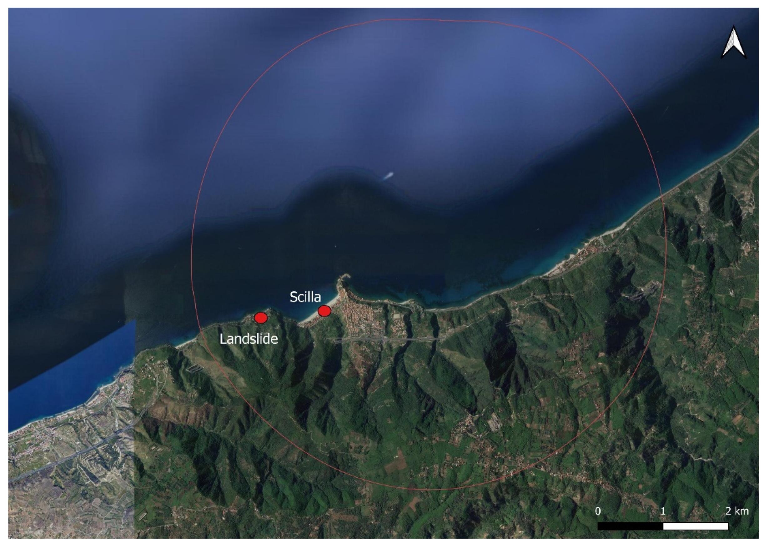
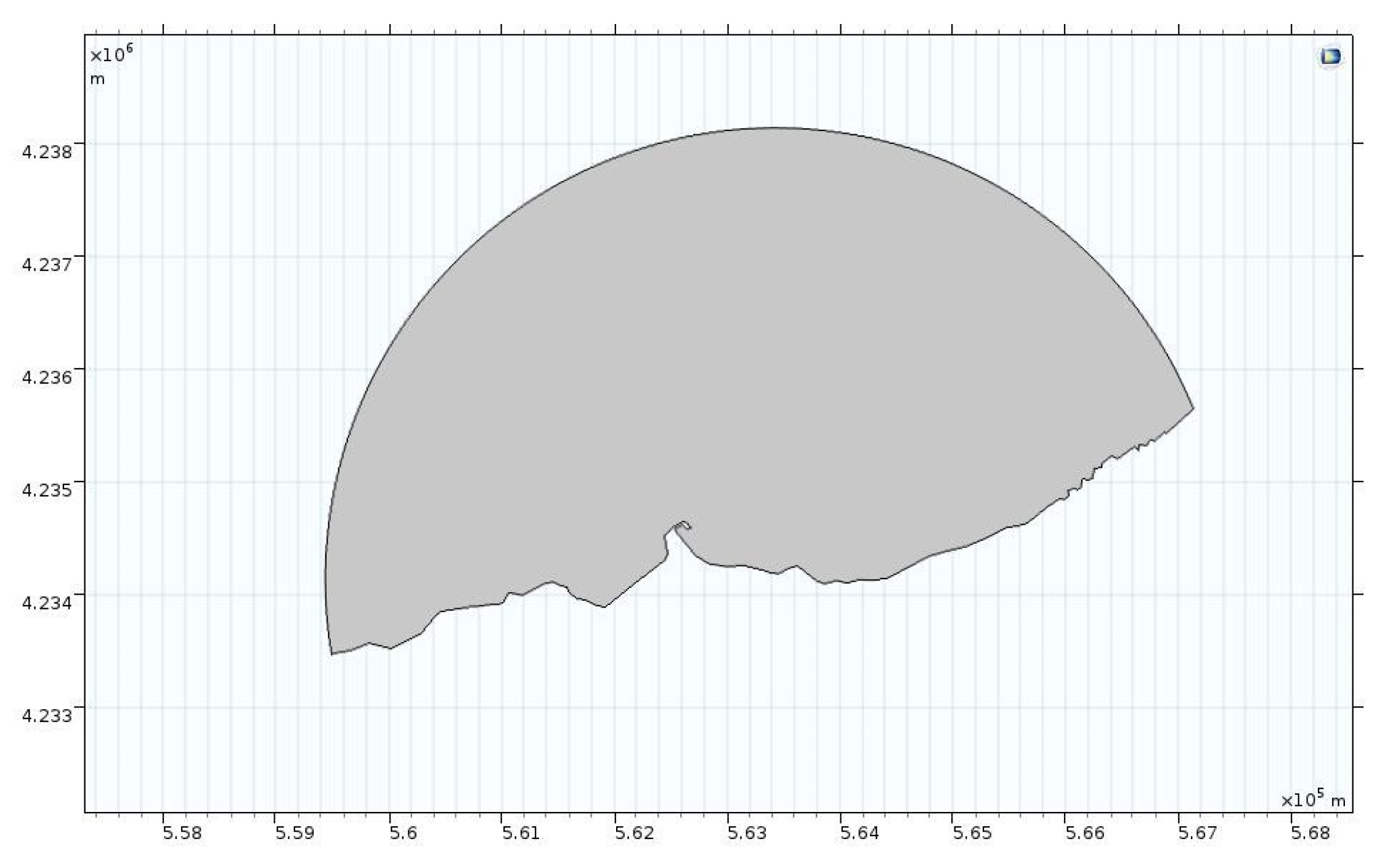
The first step to implement the model is to identify the geographic domain to be included in COMSOL, where the characteristics of the model are then assigned. For this purpose, QGIS was used, which made it possible to create, through shapefiles, the domain containing both the coastline and the circular contour that in turn encloses the affected area and the bathymetric data available (Figure 16). The reference system is WGS 84/UTM zone 33N. Using QGIS is useful because once the domain is exported in COMSOL, every point is georeferenced according to that reference system.
The domain composed is therefore purified from the area of the land not affected by the simulation and georeferencing; it can then be imported into COMSOL for modeling (Figure 17).
Regarding the source term, an array was created in MATLAB that represents the position of the landslide in the spatial dimensions x and y at various time points. The result is, therefore, a set of matrices that represent the spatial position, and in the third dimension, there is spatial variation over time. The boundary conditions used in this work are the fully reflective conditions at coastlines and a radiation condition boundary condition along the semi-circular domain, the use of which is detailed below.
The full-reflection boundary conditions can be expressed by assuming that the fluid velocity in the direction orthogonal to the boundary is zero.
Nn = 0
The radiation boundary condition can be obtained using a mathematical formulation that allows the waves that propagate toward the open boundaries to freely exit the computational domain. This condition can be easily formulated for progressive, outgoing waves (Sommerfeld, 1964; VanDongeren and Svendsen, 1997):
η t + c cos ( ϑ n ) η n = 0
The Fourier Transform of Equation (1.44) provides the radiation condition in the frequency domain (see Beltrami et al., 2001; Steward and Panchang, 2000):
N n + ikcos ( ϑ n ) N = 0
The mesh used for the numerical modeling was chosen after a convergence analysis was undertaken to find a balance between computational burdens and the detail of the result. The numerical simulation should take into account a distance between the nodes of L/10, where L is the wave length that corresponds to the higher frequency in that range of frequencies at which the energy content is significantly greater than zero and that, consequently, it is worth reproducing for the simulation. This is to ensure a minimum of 10 points for wave length.
The numerical simulation, carried out with a finite element method, uses triangular linear elements with a maximum size of 25 m and has a total DOF of 216,260.

3. Results

3.1. Landslide Movement

The simulation of the displacement of the landslide at different time points takes place, therefore, by calculating the following quantity for each spatial point and at each time point: h(x,y,t) = hf(x,y) − hl(x,y,t) (Figure 18, Figure 19 and Figure 20).

3.2. Wave Propagation

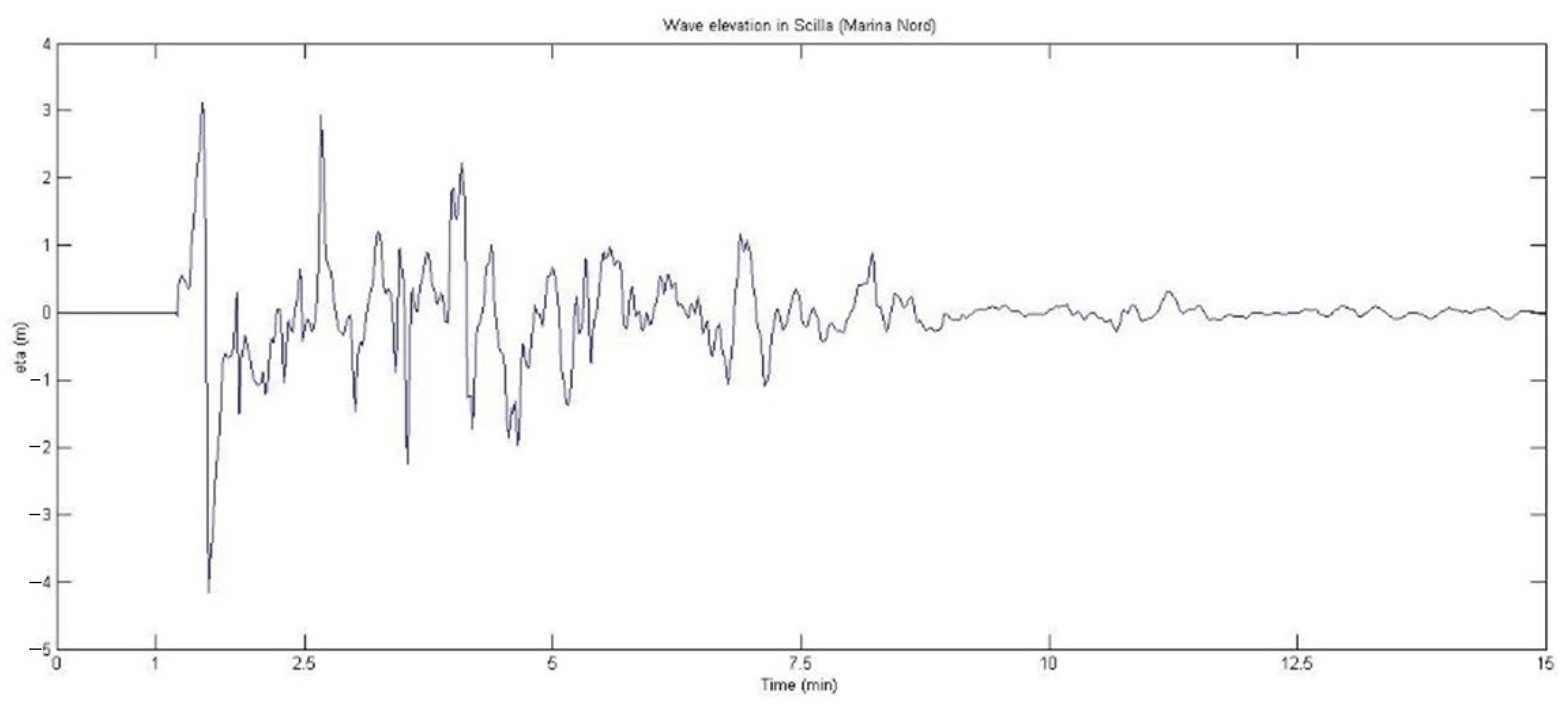
The simulation was carried out taking Δt = 2 s as the reference interval, in such a way as to have a maximum of 4000 units in time, considering a total simulation length of 8000 s (approximately 133 min). The simulation time has been chosen in such a way as to allow the waves to go completely out of the domain and not have overlap problems during the simulation itself. To these values, therefore, there correspond as many omega values between 7.85 ∗ 10−4 rad/s < ω < 3.14 rad/s and frequency values in Hz between 1.25 ∗ 10−4 Hz < f < 0.5 Hz. Once the simulation was carried out, points were then taken corresponding to the intensity of the waves generated by the tsunami in the Scilla area, as documented in historical sources (Figure 21).
The results obtained are the following:
In this study, the numerical depth-integrated model developed by Bellotti (2008) was used; in this model, the mild-slope equation is applied to reproduce the propagation of small-amplitude transient waves. The model is based on the use of the Fourier Transform to convert the time-dependent hyperbolic equation into a set of elliptic equations in the frequency domain.

4. Discussion

Regarding the hypothesis made in this study on the shape and the sliding time of the landslide necessary for the simulation, reference was made to models and simulations developed by other authors, in particular [31].
Once the landslide and its movement had been hypothesized, it was inserted into the model, and the event was simulated. The data were compared with the historical data deriving from a collection of testimonies from survivors.
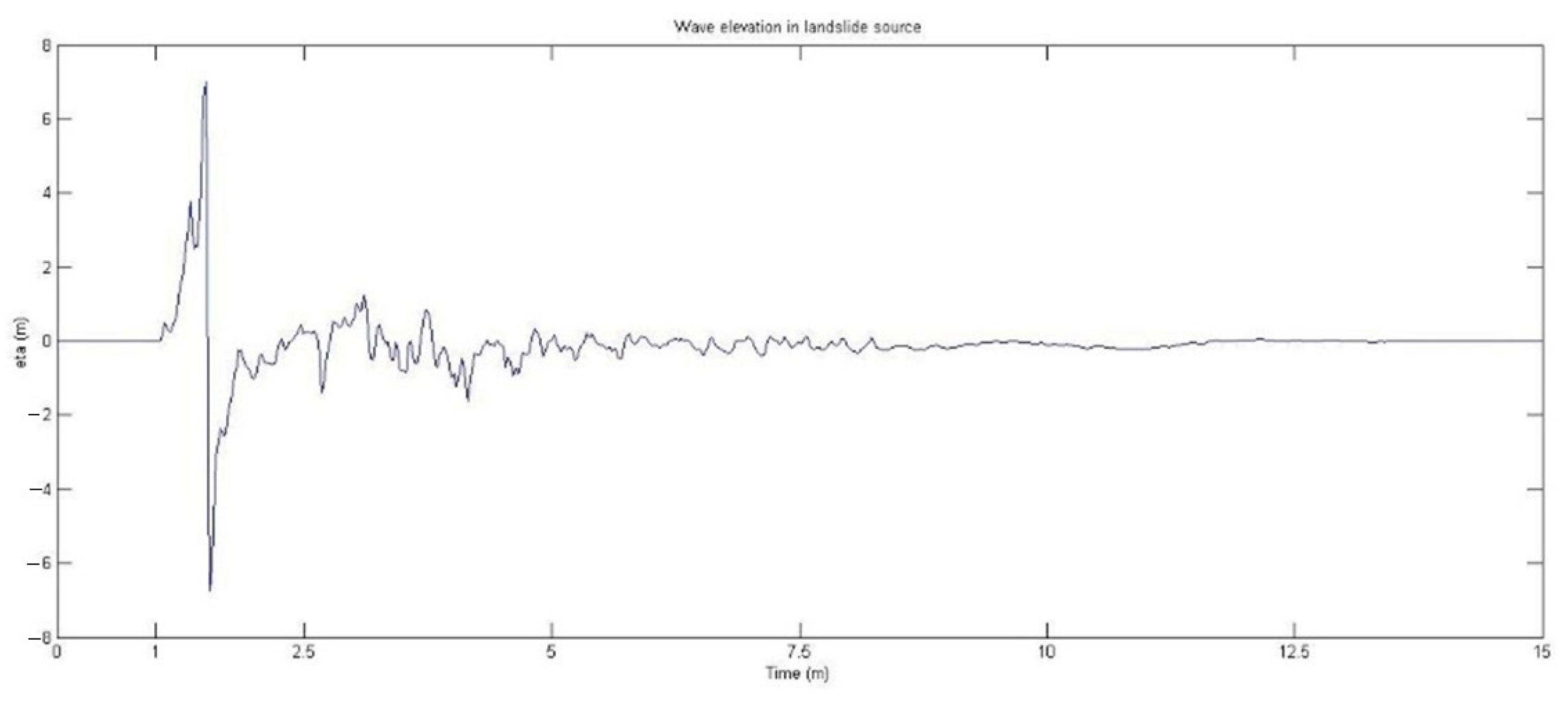
Figure 22 show free surface elevation near the source of the event, along with landslide movement in Monte Capo Pacì; (“historical sources confirm that the time sequence of the earthquake, landslide and tsunami can be seen as the first clear evidence of a landslide source for the tsunami. As a matter of fact, according to historical reconstructions, the landslide occurred about 30 min after the earthquake, and the tsunami hit the adjacent Marina Grande beach 30–60 s after the landslide”) and is characterized by one main wave triggered about 60 s after the detachment of the landslide.
Figure 23 and Figure 24 show the impact of the event in Marina Grande di Scilla, the area most severely affected by the tsunami. In the northern Scilla area, the tsunami arrived almost simultaneously at Capo Pacì after approximately 1 min. This was the area most severely hit, not only by the main wave that arrived on the coast but also by others that followed, which had less intensity but still had a disastrous effect on the coast [“three main waves hit the shore, with heights ranging from 6 to 9 m. The land was flooded for at least 100 m, with a 200 m ingression in correspondence of the Livorno stream, in the center of Marina Grande (point 7 in Figure 3b)”].
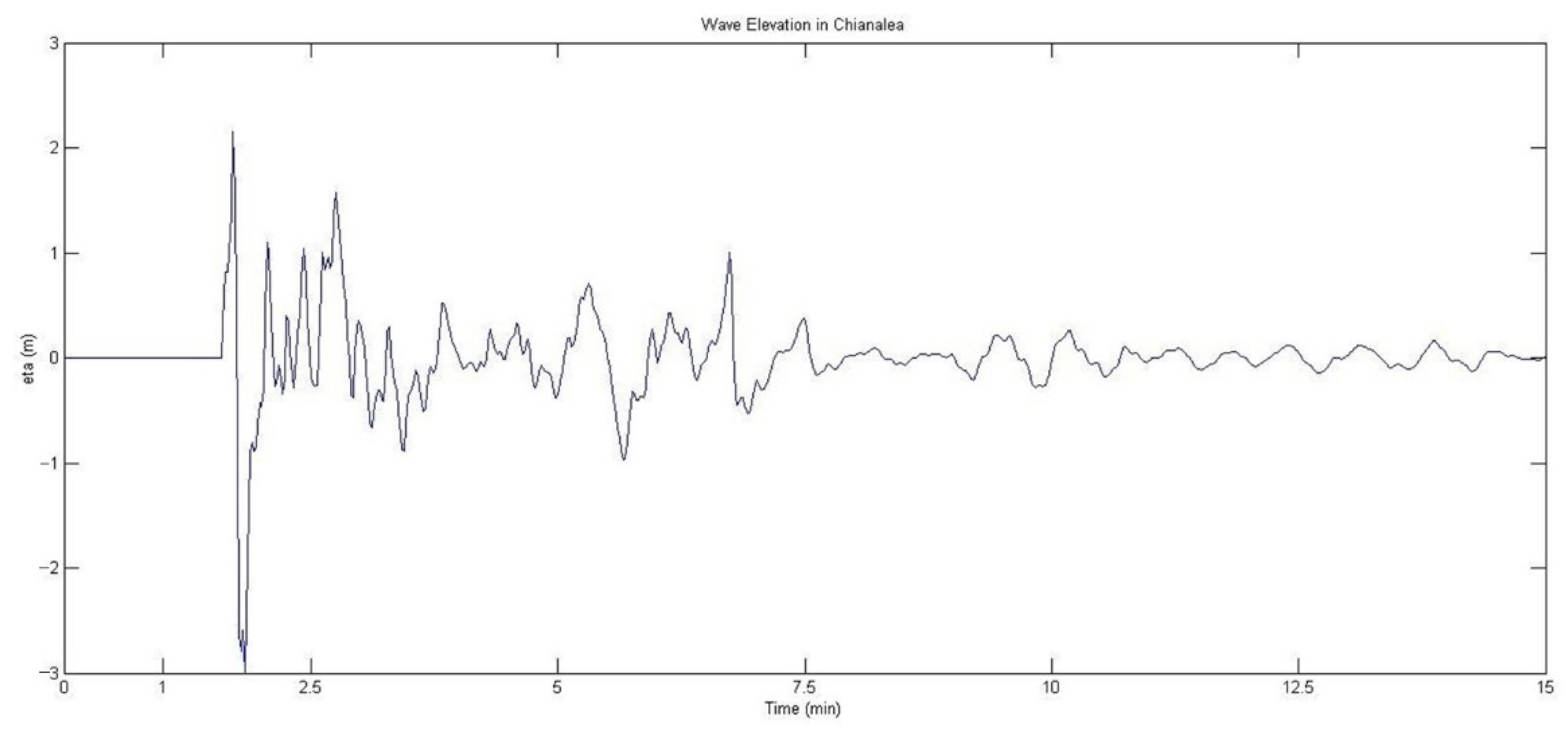
In the southern Scilla area, the main wave arrived some seconds after northern Scilla. The impact, albeit disastrous, was less strong than in the northern part. The waves following the main hit were of lower intensity, as also evidenced by the difference in the level of run-up reached between the north and the southern part of Scilla (“maximum run-up heights ranging from 6 to 9 m according to Sarconi (1784) and up to 16 m according to Minasi (1785) were recorded respectively along the south and the north of Marina Grande beach”). Figure 25 show the free surface elevation in the area of Chianalea; the main wave arrived approximately 90 sec after the tsunami was triggered, and its intensity was lower, as expected as one moves away from the source of the event and as evidenced by historical sources (“The tsunami hit the cliffs of the Scilla Castle and affected the hamlet of Chianalea (point 8, Figure 3b) on the other side of the Scilla promontory, with waves of around 3–4 m high”).

5. Conclusions

Numerical models can give important and useful information for coastal hazard assessment, in particular regarding the interaction between the tsunami and the local coastal morphology of an area, as well as with the numerous buildings that exist today. The 1783 Scilla case study demonstrated both the validation of a model that can be used to simulate possible events of this magnitude on the Calabrian coasts and the possibility of having a reliable tsunami early warning system; it also has the advantage of perfectly combining computational burdens and goodness of results. The most important feature of the model is that it can stimulate the full-frequency dispersion of the waves; the technique makes use of the Fourier Transform (with respect to the time) of the wave equation in order to obtain an elliptic equation for each component [f the wave spectrum, which are solved using a numerical model based on the finite element model.
The advantage of the model is that it can simulate the full frequency dispersion behavior more easily from a computational point of view, and it is able to incorporate the effects of landslide movements to simulate the generation of the waves. This application is presented to show the importance of applying this approach to real-life scenarios in order to predict the possible effects of an event of this magnitude on Calabrian coasts and to prepare an efficient evacuation plan for the areas affected by the flood. The important analysis of this type of historical event that could be repeated in the future must be the basis for any study aimed at developing tsunami inundation maps for the region of Calabria.

Author Contributions

Conceptualization, F.M., G.B. and G.F.; methodology, F.M., G.B. and G.F.; software, F.M.; validation, F.M., G.B. and G.F.; formal analysis, F.M.; investigation, F.M.; resources, G.B.; data curation, F.M.; writing—original draft preparation, F.M.; writing—review and editing, F.M., G.B. and G.F.; visualization, F.M., G.B. and G.F.; supervision, G.B.; project administration, G.B. All authors have read and agreed to the published version of the manuscript.

Funding

This research received no external funding.

Institutional Review Board Statement

Not applicable.

Informed Consent Statement

Not applicable.

Acknowledgments

Special thanks go to Giorgio Bellotti from the University of Roma Tre for the precious advice and suggestions given, which were necessary for the development of this study, and the immense goodwill shown in our collaboration.

Conflicts of Interest

The authors declare no conflict of interest.

References

  1. Grilli, S.T.; Vogelmann, S.; Watts, P. Development of a 3D numerical wave tank for modeling tsunami generation by underwater landslides. Eng. Anal. Bound. Elem. 2002, 26, 301–313. [Google Scholar] [CrossRef]
  2. Grilli, S.T.; Watts, P. Modeling of waves generated by a moving submerged body. Applications to underwater landslides. Eng. Anal. Bound. Elem. 1999, 23, 645–656. [Google Scholar] [CrossRef]
  3. Tinti, S.; Maramai, A.; Graziani, L. The new catalogue of Italian tsunamis. Nat. Hazards 2004, 33, 439–465. [Google Scholar] [CrossRef]
  4. Schambach, L.; Grilli, S.T.; Tappin, D.R.; Gangemi, M.D.; Barbaro, G. New simulations and understanding of the 1908 Messina tsunami for a dual seismic and deep submarine mass failure source. Mar. Geol. 2020, 421, 106093. [Google Scholar] [CrossRef]
  5. Schambach, L.; Grilli, S.T.; Tappin, D.R.; Gangemi, M.D.; Barbaro, G. Response to: Comment on “New simulations and understanding of the 1908 Messina tsunami for a dual seismic and deep submarine mass failure source”. Mar. Geol. 2021, 442, 106636. [Google Scholar] [CrossRef]
  6. Minasi, G. Continuazione ed Appendice Sopra I Tremuoti Descritti Nella Relazione Colla Data di Scilla de 30 Settembre 1783, con Altro che Accadde in Progresso; Di Stefano G.: Messina, Italy, 1785. (In Italian) [Google Scholar]
  7. Sarconi, M. Istoria de’ Fenomeni del Tremuoto Avvenuto nelle Calabrie e nel Valdemone Nell’anno 1783; Reale Accademia delle Scienze e delle Belle Lettere di Napoli: Napoli, Italy, 1784. (In Italian) [Google Scholar]
  8. Vivenzio, G. Historia dei Tremuoti Avvenuti Nella Provincia di Calabria Ulteriore e nella citta ‘di Messina Nell’anno 1783; Stamperia Regale: Napoli, Italy, 1788. (In Italian) [Google Scholar]
  9. Hamilton, W. Relazione Dell’ultimo Terremoto Delle Calabrie e della Sicilia; Stamperia della Rovere: Firenze, Italy, 1783. (In Italian) [Google Scholar]
  10. De Lorenzo, A. Memorie da Servire alla Storia Sacra e Civile di Reggio e delle Calabrie; Stamperia Siclari: Reggio Calabria, Italy, 1877; Volume I. [Google Scholar]
  11. Zaniboni, F.; Armigliato, A.; Tinti, S. A numerical investigation of the 1783 landslide induced catastrophic tsunami in Scilla, Italy. Nat. Hazards 2016, 84, 455–470. [Google Scholar] [CrossRef]
  12. Tinti, S.; Tonini, R. The UBO-TSUFD tsunami inundation model: Validation and application to a tsunami case study focused on the city of Catania, Italy. Nat. Hazards Earth Syst. Sci. 2013, 13, 1795–1816. [Google Scholar] [CrossRef] [Green Version]
  13. Zaniboni, F.; Pagnoni, G.; Gallotti, G.; Paparo, M.A.; Armigliato, A.; Tinti, S. Assessment of the 1783 Scilla landslide-tsunami effects on Calabria and Sicily coasts through numerical modeling. Nat. Hazards Earth Syst. Sci. 2019, 19, 1585–1600. [Google Scholar] [CrossRef] [Green Version]
  14. Bellotti, G.; Cecioni, C.; De Girolamo, P. Simulation of small-amplitude frequency-dispersive transient waves by means of the mild-slope equation. Coast. Eng. 2008, 55, 447–458. [Google Scholar] [CrossRef]
  15. Bellotti, G.; Di Risio, M.; De Girolamo, P. Feasibility of Tsunami Early Warning Systems for small volcanic islands. Nat. Hazards Earth Syst. Sci. 2009, 9, 1911–1919. [Google Scholar] [CrossRef] [Green Version]
  16. Bellotti, G.; Beltrami, G.M.; De Girolamo, P. Internal generation of waves in 2D fully-elliptic mild-slope equation FEM models. Coast. Eng. 2003, 49, 71–81. [Google Scholar] [CrossRef]
  17. Barbaro, G.; Petrucci, O.; Canale, C.; Foti, G.; Mancuso, P.; Puntorieri, P. Contemporaneity of floods and storms. A case study of Metropolitan Area of Reggio Calabria in Southern Italy. In Proceedings of the 3rd International Symposium New Metropolitan Perspectives Smart Innovation, Systems and Technologies, Reggio Calabria, Italy, 22–25 May 2020; Volume 101, pp. 614–620. [Google Scholar] [CrossRef]
  18. Barbaro, G.; Foti, G.; Nucera, A.; Barillà, G.C.; Canale, C.; Puntorieri, P.; Minniti, F. Risk mapping of coastal flooding areas. Case studies: Scilla and Monasterace (Italy). Int. J. Saf. Secur. Eng. 2020, 10, 59–67. [Google Scholar] [CrossRef]
  19. Barbaro, G.; Gangemi, M.D.; Foti, G. An agent-based tsunami alert system. In Proceedings of the 18th Workshop “From Objects to Agents”, Scilla, Italy, 15–17 June 2017; Volume 1867, pp. 102–107. [Google Scholar]
  20. Canale, C.; Barbaro, G.; Petrucci, O.; Fiamma, V.; Foti, G.; Barillà, G.C.; Puntorieri, P.; Minniti, F.; Bruzzaniti, L. Analysis of floods and storms: Concurrent conditions. Ital. J. Eng. Geol. Environ. 2020, 1, 23–29. [Google Scholar] [CrossRef]
  21. Foti, G.; Barbaro, G.; Bombino, G.; Fiamma, V.; Puntorieri, P.; Minniti, F.; Pezzimenti, C. Shoreline changes near river mouth: Case study of Sant’Agata River (Reggio Calabria, Italy). Eur. J. Remote Sens. 2019, 52, 102–112. [Google Scholar] [CrossRef]
  22. Minniti, F.; Foti, G.; Barbaro, G. Analysis of areas inundated by tsunamis induced by earthquakes and landslides in the region of Calabria, Italy. In Proceedings of the 12th International Conference on Risk Analysis and Hazard Mitigation, Online. 23–25 June 2020; Volume 129, pp. 135–146. [Google Scholar] [CrossRef]
  23. Baratta, M. I Terremoti d’Italia. Saggio di Storia, Geografia e Bibliografia Sismica Italiana; F.lli Boccal: Turin, Italy, 1901. (In Italian) [Google Scholar]
  24. Tinti, S.; Guidoboni, E. Revision of the tsunamis occurred in 1783 In Calabria and Sicily (Italy). Sci Tsunami Hazards 1988, 6, 17–22. [Google Scholar]
  25. Graziani, L.; Maramai, A.; Tinti, S. A revision of the 1783–1784 Calabrian (southern Italy) 5 tsunamis. Nat. Hazards Earth Syst. Sci. 2006, 6, 1053–1060. [Google Scholar] [CrossRef] [Green Version]
  26. Tinti, S.; Maramai, A.; Graziani, L. The Italian Tsunami Catalogue (ITC), Version 2. 2007. Available online: http://www.ingv.it/servizi-e risorse/BD/catalogotsunami/catalogo-degli-tsunami-italiani (accessed on 15 October 2021).
  27. Tinti, S.; Pagnoni, G.; Zaniboni, F. The landslides and tsunamis of the 30th of December 2002 in Stromboli analyzed through numerical simulations. Bull. Volcanol. 2006, 68, 462–479. [Google Scholar] [CrossRef]
  28. Cecioni, C.; Bellotti, G. Inclusion of landslide tsunamis generation into a depth integrated wave model. Nat. Hazards Earth Syst. Sci. 2010, 10, 2259–2268. [Google Scholar] [CrossRef] [Green Version]
  29. Cecioni, C.; Bellotti, G. Modeling tsunamis generated by submerged landslides using depth integrated equations. Appl. Ocean. Res. 2010, 32, 343–350. [Google Scholar] [CrossRef]
  30. Mazzanti, P. Studio integrato subaereo-subacqueo di frane in ambiente costiero: I casi di Scilla (RC) e del lago di Albano (RM). G. Geol. Appl. 2008, 8, 245–261. [Google Scholar]
  31. Mazzanti, P.; Bozzano, F. Revisiting the February 6th 1783 Scilla (Calabria, Italy) landslide and tsunami by numerical simulation. Mar. Geophys Res. 2011, 32, 273–286. [Google Scholar] [CrossRef]
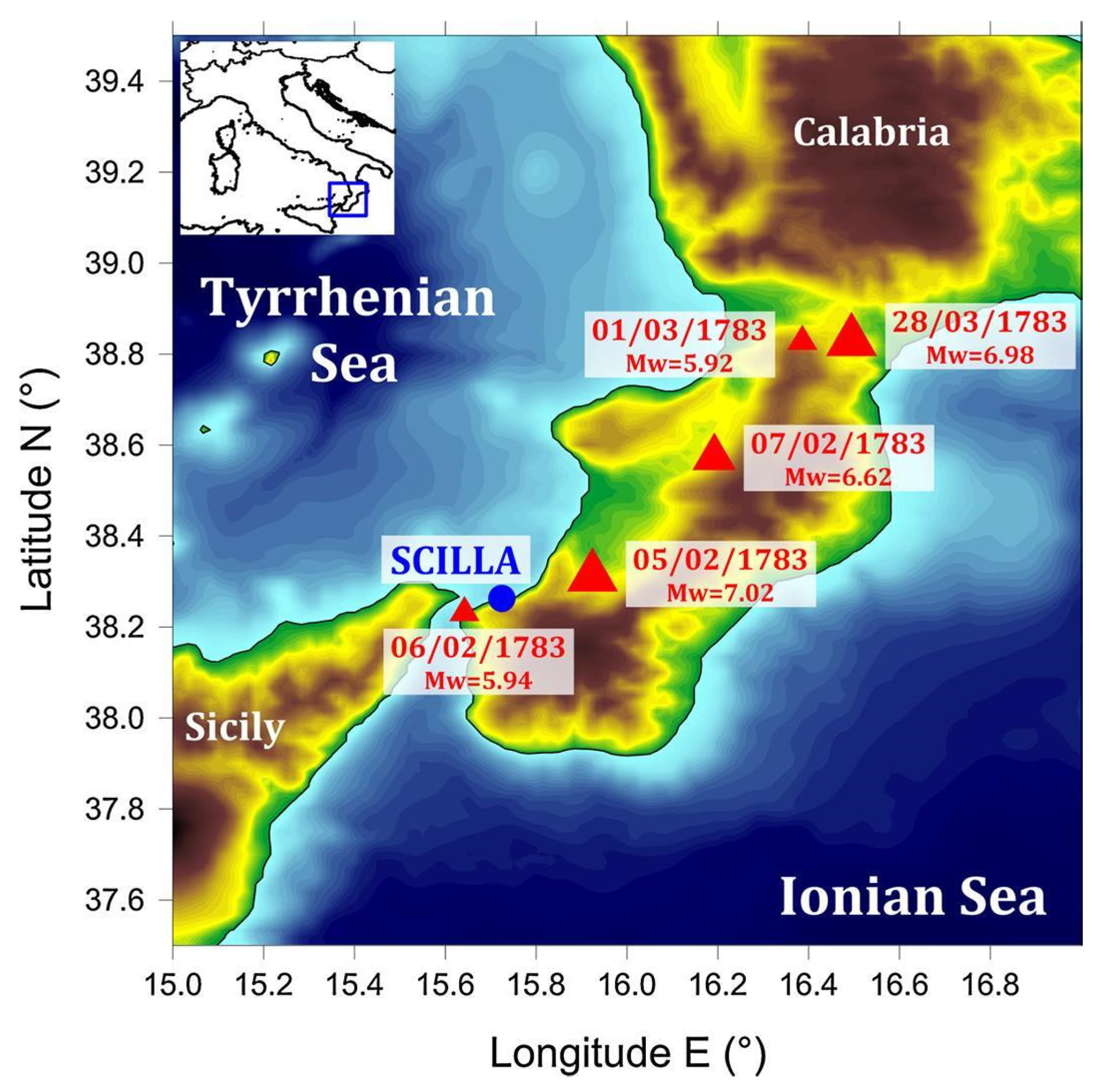
Figure 1. Epicenters (red triangles), dates and magnitudes of the five strongest earthquakes affecting Calabria during 1783 (Zaniboni et al., 2016).
Land 11 00069 g001
Figure 2. Location of the landslide triggered by the earthquake followed by the tsunami (source QGIS).
Land 11 00069 g002
Figure 3. (a) Topo-bathymetry of the region where the slide occurred. (b) Satellite image from Google Earth of Scilla, with Marina Grande and Chianalea (Zaniboni et al, 2016).
Land 11 00069 g003
Figure 4. Inundation distance and run-up height in some of the locations along the coast. (r) Historically reported, (c) Computed from the reported inundation distance (Gerardi et al. 2008), (n.a.) data not available (Mazzanti and Bozzano, 2011).
Land 11 00069 g004
Figure 5. Summary of evidence of the 1783 tsunami in Calabria and Sicily, with the exclusion of local effects in the area of Scilla.
Land 11 00069 g005
Figure 6. Sketch representing the main variables involved in the analytical model.
Land 11 00069 g006
Figure 7. Methodology used in the study.
Land 11 00069 g007
Figure 8. Domain of IGM bathymetry (purple dots) for the event of 1783.
Land 11 00069 g008
Figure 9. Two-dimensional plane view of meshgrid interpolating bathymetric data.
Land 11 00069 g009
Figure 10. Three-dimensional plane view of meshgrid interpolating bathymetric data.
Land 11 00069 g010
Figure 11. Identification of the subdomain affected by the landslide in QGIS (red dashed rectangle).
Land 11 00069 g011
Figure 12. Two-dimensional plane view of the landslide geometric shape.
Land 11 00069 g012
Figure 13. Three-dimensional plane view of the landslide geometric shape.
Land 11 00069 g013
Figure 14. Two-dimensional plane view of the ellipsoidal bathymetric subdomain.
Land 11 00069 g014
Figure 15. Three-dimensional plane view of the ellipsoidal bathymetric subdomain.
Land 11 00069 g015
Figure 16. QGIS shapefile representing domain boundaries (red circle).
Land 11 00069 g016
Figure 17. Scilla computational domain purified from the part of the land (source COMSOL).
Land 11 00069 g017
Figure 18. Landslide modeling at time T = 15 s.
Land 11 00069 g018
Figure 19. Landslide modeling at time T = 45 s.
Land 11 00069 g019
Figure 20. Landslide modeling at time T = 80 s.
Land 11 00069 g020
Figure 21. Points where the elevation of the wave was evaluated. In green, is the area of Chianalea; in red, Scilla Sud; in orange, Scilla Nord. The arrow indicates the position of the landslide and the point where the wave elevation was evaluated (source QGIS).
Land 11 00069 g021
Figure 22. Free surface elevation obtained from the depth-integrated model in Monte Capo Pacì (the landslide source).
Land 11 00069 g022
Figure 23. Free surface elevation obtained from the depth-integrated model in Scilla Marina Grande Nord.
Land 11 00069 g023
Figure 24. Free surface elevation obtained from the depth-integrated model in Scilla Marina Grande Sud.
Land 11 00069 g024
Figure 25. Free surface elevation obtained from the depth-integrated model in Scilla Chianalea.
Land 11 00069 g025
Table 1. Meshgrid features interpolating bathymetric data.
Δx (m)Δy (m)NxNyXmin (m)Xmax (m)Ymin (m)Ymax (m)
1010250026505.4730 × 1055.7247 × 1054.2229 × 1064.2494 × 106
Table 2. Meshgrid features of the bathymetric subdomain.
Δx (m)Δy (m)NxNyXmin (m)Xmax (m)Ymin (m)Ymax (m)
1010371585.6105 × 1055.6150 × 1054.2340 × 1064.2356 × 106
Table 3. Time features of the landslide displacement in its subaerial phase.
Total Time of Displacement (s)ΔT (s)Nt
300.579
Table 4. Time features of the landslide displacement in its submerged phase.
Total Time of Displacement (s)ΔT (s)Nt
400.479
Publisher’s Note: MDPI stays neutral with regard to jurisdictional claims in published maps and institutional affiliations.