Article

Comparing Nonlinear and Threshold Effects of Bus Stop Proximity on Transit Use and Carbon Emissions in Developing Cities

School of Urban Planning and Design, Peking University, Shenzhen 518055, China
*
Author to whom correspondence should be addressed.
Land 2023, 12(1), 28; https://doi.org/10.3390/land12010028
Submission received: 15 November 2022 / Revised: 18 December 2022 / Accepted: 19 December 2022 / Published: 22 December 2022

Abstract

:
Transit proximity is impactful in providing congestion relief and carbon emissions reduction only within a certain range, while the effective ranges to achieve different policy goals might be distinct. Comparing the impact boundaries of transit proximity on transit use and carbon emissions offers insights for planners to coordinate multidimensional goals more efficiently, but few studies have conducted this comparative analysis. Using 2019 travel data in Zhongshan, this study employed a gradient-boosting decision tree to quantify the nonlinear and threshold effects of bus stop proximity on transit use and commuting-related carbon emissions. Results indicate that the relative impact of bus stop proximity in developing cities is significantly lower than that in developed cities. We found a weaker association between bus stop proximity and carbon emissions than between bus stop proximity and transit use in developing cities. The impact thresholds of bus stop proximity on carbon emissions and the probability of commuting via transit are distinct, and both are lower than China’s current national standards. The findings suggest that some ranges of proximity to bus stops across a developing city can help reduce carbon emissions but cannot help relieve congestion. Most importantly, we found that, due to disparities in the impact boundary on different policy variables and the corresponding analysis criteria, the calculated stop coverage rate varies dramatically. This finding challenges the validity of using national criteria to guide transportation planning and assess land use performance.

1. Introduction

Rapid motorization in urban areas has produced undesirable consequences such as road congestion and carbon emissions. Planning authorities typically consider land use strategies to be a measure of congestion relief and carbon emission reduction [1,2]. Concerning land use patterns and features of the built environment, proximity to transit remains a key area of focus in urban planning [3,4]. In 2012, the Chinese central government proposed station coverage rates as one of the indicators in transit-priority strategies to manage and evaluate city development. This indicator quantifies the extent to which citizens are proximate to transit under present land use patterns and is viewed as a fundamental standard of transit construction in most local zoning codes. Making full use of transit proximity effects in urban development can improve land use performance by mitigating congestion and carbon emissions [5,6].
Several intriguing questions emerge for planners: How far does the impact of a transit stop on mode choice and carbon emissions extend? How proximate is enough to increase transit usage and reduce carbon emissions efficiently? This impact boundary can be used to determine the station catchment area. Conventional wisdom provided by the American Public Transportation Association advises using a five-minute walking distance as the limit [7]. China’s national code for transport planning on urban roads adopted a 500-m buffer distance. However, these two approaches may not be suitable for current development in light of subsequent economic growth and time value uplift. Some studies predefined a radius of 400, 600, or 800 m [8] and were criticized for probable bias [9]. Other scholars have computed the impact boundary by investigating the nonlinear effects of transit proximity (that is, the marginal proximity effects are not constant). Changes in transit proximity may be ineffective after exceeding a certain threshold, which can be depicted as threshold effects [10].
Although previous studies offer ample evidence supporting the nonlinear and threshold effects of transit proximity in developed cities, context-specific research is still needed in developing cities. The relative contribution and changing pattern of transit proximity could be distinct, considering the differential features of developing and developed cities regarding transportation systems [11]. Moreover, scholars often concentrate on the impact of transit proximity on single policy variables, overlooking varying nonlinear relationships that affect many different policy purposes [10]. Diverse impact boundaries might be identified with varied goals; the risk is that an inappropriate threshold may lead to a suboptimal standard being drawn for urban planning. Furthermore, the performance assessment of land use based on such a standard is likely to be biased. For this reason, it is necessary to compare the threshold effects of bus stop proximity across different policy purposes for efficient transport planning and precise land use evaluation.
Using the travel survey data in Zhongshan, China, this study applies a gradient boosting decision tree (GBDT) to investigate nonlinear and threshold effects on transit use and carbon emissions with regard to commuters’ journeys to work. It fills the aforementioned two research gaps in the literature by answering two questions: (1) How important is bus stop proximity in promoting transit use and reducing carbon emissions in developing cities? (2) How different are the nonlinear and threshold effects of bus stop proximity on transit use and carbon emissions?
The paper is organized as follows. Section 2 reviews bus stop proximity impacts on transit use and carbon emissions. Section 3 introduces the methodology, and Section 4 presents empirical results. Finally, Section 5 provides a conclusion and policy recommendations.

2. Literature Review

Proximity to transit, also known as distance to transit, is a key variable in the built environment. It can be measured either spatially by the Euclidean distance and street distance to a given transit stop [12] or temporally by the walking time and trip duration to a stop [13]. Transit route density, the distance between transit stops, and the total count of transit stations per unit area are lesser indicators of proximity to transit [3]. Proximity to transit is proven to be closely related to travel behaviors, especially transit use. Zhang attributes station proximity effects on transit use to three factors [14]. First, space allocation near rail stations and bus stops tends to be more transit-oriented. Second, increased safety, comfort, and convenience of transit services are perceived under proximity effects. Third, proximity to transit captures the influence of latent factors affecting mode choice, such as trip distance.
The connection between commuting via transit and proximity to transit has been substantially studied within various contexts and methodologies. Shen et al. utilize nested logic to show that a 1 km increase in distance to the nearest rail station lowers the odds ratio between transit use and car driving by 0.07 [15]. Similar models have been employed in the work of Zhao, Zhang, and Ao et al. in Beijing, Boston, and Sichuan, respectively [14,16,17]. Elsewhere, structural equation models and principal component analysis demonstrated that proximity to transit indirectly facilitates transit use by shortening the trip distance, which verifies the third mechanism proposed by Zhang [14]. Other research investigates the heterogeneity of proximity effects. For instance, the relative impact strength of transit proximity varies by income, career, gender, age, household kind, and location [18,19,20,21,22]. Station features, as well as macro-level transportation demand management and land use patterns, can also cause variation in elasticity [16,23,24]. Additionally, several studies have controlled for self-selection and personal attitudes toward transit to illuminate the causal relationship between transit proximity and transit taking [25,26].
More importantly, the relationship between proximity to transit and transit use has been found to be nonlinear. The association appears only with a certain range of transit proximity. Viggiano et al. analyzed the cumulative distribution of transit users’ straight-line access distance and found that transit use sharply declines once the proximity to a bus stop exceeds 0.2 miles [24]. Guerra et al. separated station areas into several parts, incorporating a series of dummy variables for each part [27]. Their results demonstrated that the proximity effects on transit use are not significant when a commuter is outside 0.5 miles of a bus stop; therefore, the influence of the bus stop only extends to that distance. Ding et al. applied GBDT, using Beijing’s data, to illustrate that proximity to rail stations generates the strongest impacts on transit commuting probability within an 800-m buffer, with trivial influences exerted outside that buffer [28].
In addition to the propensity to use transit, proximity to transit affects commuting distance, vehicle ownership, travel speed, and other travel behaviors [29,30,31], which collectively affect commuting-related carbon emissions. Plentiful evidence exists at the disaggregated level, provided by structural equation models that explain the pathway between transit proximity and carbon emissions through commuting mode choice as well as car ownership [6,32,33]. Travel behaviors, such as vehicle type choice and trip frequency, are also mediated by the effects of proximity on carbon emissions [34,35]. Considering direct and indirect impacts, a study by Ma et al. suggests that a one-unit decrease in distance to a rail station decreases the carbon emissions from commuting by 0.074 [6]. This causality is explained with quasi-experimental analysis [33,36,37].
As a combined outcome of transit use and other travel behaviors, carbon emissions also respond to transit proximity in a nonlinear pattern [30,38,39,40]. Log-linear and quadratic functions are two ways to analyze predefined nonlinear relationships, but they might be inaccurate if the nonlinear pattern is irregular [38]. In contrast, the threshold effect is a less commonly studied but more salient nonlinear influence. For instance, using survey data in the United States Twin Cities region, Wu et al. investigate the nonlinear effects of transit proximity on travel-related carbon emissions and find a threshold effect. As long as proximity to the nearest stop is under 0.5 miles, carbon emissions rise sharply as the distance to the stop increases. However, the slope becomes much more gentle after the distance exceeds 0.5 miles; the marginal effects rapidly diminish beyond a distance of 1 mile [41]. The authors suggest planning multifamily housing along select public transit routes, per this impact boundary, to reduce environmental pollution.
Most studies have tested the nonlinear and threshold effects of transit proximity in developed countries; in comparison, insights from developing cities have been neglected. Especially with regard to the association between transit proximity and carbon emissions, current findings are based on cities with rail transit and do not transfer neatly to developing cities with only bus transit. This is for three primary reasons. First, the functions and components of a given transit system could affect the relative importance and impact boundary of transit proximity. A rail station catchment area is usually larger than a bus stop [24]. The buffer distance around a bus stop could vary with different intermodal relations [42,43]. Bus stops provide feeder services for rail transit in developed cities, but they provide major public transit services in developing cities. Therefore, individuals in developing cities could exhibit lower tolerance and stricter requirements based on bus stop proximity.
Second, travel by electric bicycle or motorcycle is low-cost with high door-to-door accessibility, which suits citizens with low but growing incomes. These travel modes are becoming increasingly prevalent in developing cities and can make commuters more sensitive to bus stop proximity [18]. Third, Chinese urban development prefers megacities and densely constructed metropolitan areas where a car-free lifestyle can be more easily sustained. However, most developing cities are characterized by inadequate infrastructure and low-quality transit service [11], which can weaken the proximity and threshold effects of bus stops. Accordingly, new insights into the nonlinear and threshold effects of transit proximity in developing cities merit further discussion.
Another gap in the literature arises from its extensive focus on proximity effects concerning single policy variables. This overlooks the fact that the impact threshold can be different when various policy purposes are considered. Wu et al. establish a proximity boundary of 1 mile to minimize carbon emissions. Whether proximity to rail stations lower than 1 mile is influential in promoting transit use remains unanswered in this study [41]. Still, this question is important for the following three reasons: First, carbon emission capture proximity effects on transit use, as well as trip distance and other variables. Even if proximity to a bus stop is insufficient to facilitate transit use, as long as it reduces trip distances, travel-related carbon emissions could still decrease. As a result, the impact boundary might be diverse. Second, nonlinear proximity effects on transit use and carbon emissions arise from different mechanisms. Galster summarizes five behavioral mechanisms for nonlinear and threshold effects: collective socialization, gaming, tolerance, contagion, and diminishing returns. The nonlinear proximity effects on transit usage mainly derive from bus stop proximity reducing transit commuting costs at a diminishing marginal rate [10]. Carbon emissions reflect the intensity of human activities and the related proximity effects stemming from individual interactions, accounting for gaming as well as contagion with nearby environments and social groups. Variations in individual behavioral mechanisms could give rise to different impact boundaries. Finally, transportation planning serves multiple policy goals but suffers from a lack of clear indicators to guide its development [4]. Recommendations for built environment features based on studies with a single objective might be useful in reducing pollution, but they may have less utility in congestion relief. Comparative analysis of the threshold effects of transit proximity for different policy purposes will help to elevate the efficiency of urban planning guidance, thereby achieving greater sustainability and livability.
In summary, although previous studies offer valuable insights about transit proximity effects on transit use and carbon emissions, empirical analysis of developing cities is scarce. The threshold effects of transit proximity on different policy purposes merit further explanation. This study contributes to the existing literature investigating the nonlinear effects of transit proximity in two ways. First, this study procures evidence from developing cities with bus transit systems but no rail systems. Second, it compares the impact boundary of transit proximity on transit use and carbon emissions, highlighting that variable standards of land development should be recommended to achieve different policy aims.

3. Methodology

3.1. Data and Variables

We selected Zhongshan city, a prefectural city in China, to study the nonlinear and threshold effects of bus stop proximity on transit use and commuting-related carbon emissions in the central city and suburban areas (see Figure 1). Zhongshan is polycentric, lacking a strong city-level center. The central city houses 1,000,000 permanent residents, and the suburban area houses 3,000,000. Under China’s national official standards, Zhongshan is considered a developing city, lacking the qualifications to build rail transit. Accordingly, bus transit is the primary system of public transportation. Zhongshan also has a high vehicle volume, with 1,200,000 electric bikes, 600,000 motorcycles, and 1,000,000 private cars.
This study uses three datasets: (1) travel survey data, (2) land use data, and (3) Internet map data. The sample used in this analysis was collected from a travel survey conducted in April 2019, which assessed 45,700 individuals in 1337 traffic analysis zones at a sample rate of 1.5%. After data cleaning, 31,155 valid commute records were obtained, with 8411 in the central city and 22,744 in suburban areas. The survey records participants’ trip origin and destination, commuting mode, and demographics. According to the survey, the modal split of cars, electric bicycles, motorcycles, buses, walking, and bicycles are 25.8%, 21.8%, 38.6%, 2.1%, 2.7%, and 9.0%, respectively.
The land use data were provided by the Bureau of Land Management in Zhongshan. It consists of Zhongshan’s land use patterns and road distribution in 2019. Nine land uses could be identified with this dataset: public administration and public service, commercial service, green spaces and plazas, construction use, industrial use, residential use, transportation use, public facilities, and warehousing.
The Internet map data obtained from Baidu Map includes the street distance for each trip, the heatmap image data, and the location of each bus stop. Baidu Map is a product similar to Google Maps, offering users location-based services, including place inquiry and route search. In 2019, Baidu Map ranked as the most-used search engine in China, with the number of users reaching 400 million. Baidu Map is also officially recommended for its information services by local governments and transit operators in Zhongshan. Moreover, the data in Baidu Map is open to the public through its application programming interface (API), which has been extensively used in previous studies [38,44,45].
Baidu Map’s “route search” module outputs travel information according to the input origin (O) and destination (D) of residents’ trips. For input transport modes, the information includes travel distance. We designed a program to automatically input the O and D information into Baidu Map to obtain the street distance of 31,155 trips. Compared with ArcGIS, Baidu Map uses the most up-to-date traffic information to calculate the street distance, making it more intelligent [46] and more widely adopted in planning studies [18,47].
The heatmap raster data reports the real-time relative magnitude of the density scale based on the number of users. Because Baidu Map reaches more than 28% of the population, many scholars use the heat value as a proxy for population density when census data cannot be resolved to a small geographic area. After vectorizing the heatmap images and reclassifying the data into several scales, researchers usually aggregate the categorized data within a 1 km buffer around the house for each observation and obtain a scale value approximating density. Zhang et al. built a regression between the scale value and the “true” density value in the yearbook at the sub-district level and showed that the R-squared (R2) is around 0.7, which suggests that the heatmap data fits the density well [45]. Therefore, we used the heatmap data to generate an intensity index as a proxy for density in a similar way. The heatmap image data were extracted from the Baidu Map API at the 8 × 8 m grid level between Tuesday, 18 August, and Thursday, 20 August 2020.
The location data showed the latitude and longitude of each bus stop and was collected on 6 October 2020. The location information of points of interest (POI) is stable and reliable after several years of self-adjustment and user feedback. The location data cover 2238 bus stops, which are identical to the lists obtained from the internet. The number of bus stops recorded by the city archive in Zhongshan is 2124, which is slightly less than that in Baidu Map. Considering that the city archive might not consider the adjustment of bus routes and stops within the year, the difference is acceptable, and the locations obtained from Baidu Map can be considered reliable.
The dependent variables are transit use and carbon emissions during participants’ commutes. Because congestion relief relies on private motorized travelers shifting to transit, only transit taking, car driving, electric bike riding, and motorcycle riding are considered when accounting for the effects of bus stop proximity on transit use. All valid samples are considered when accounting for the carbon emissions from commuting.
Emissions from commuting are calculated using commuting distance Di multiplied by emission rate Ri. The commuting distance Di refers to the street distance for each travel mode. This calculation was proposed in the 2006 IPCC Guidelines for National Greenhouse Gas Inventories [48] and is commonly utilized in transportation research. The emissions factor refers to the amount of carbon dioxide emitted per traveler per kilometer. Previous studies used emission factors from diverse sources, including departments in the United States, the United Kingdom, and the European Council (EC) [32,33,41,44]. Because the study area in Ao et al.’s work share similarities to the transport modes with Zhongshan [32], we chose to use their emissions factors in this work. The emission rate Ri for each corresponding mode is presented in Table 1.
In addition to proximity to a given bus stop, the independent variables include built environment features and demographics. Bus stop proximity is measured by the straight-line distance to the nearest bus stop. An entropy index is computed based on the land use data using the following equation to assess the mixture of nine land uses:
i = 1 s ( p i ) l n ( p i ) l n ( s )
where s is the number of land uses, and pi is the proportion of the area in the ith land use. Employment density is indirectly measured by the average values of an intensity index derived from heatmap data collected at 10 a.m., 11 a.m., 3 p.m., and 4 p.m. Population density is indirectly measured by the average values generated from heatmap data collected at 11 p.m. and 12 a.m. Employment density and population density are averaged within a buffer of 1 km buffer around participants’ houses. Road density is indicated by the street length per square kilometer around the house. Distance to the nearest city center is also controlled. Demographic data covers gender, income level, educational background, family size, and the number of children. Table 2 presents the definitions and statistics of the aforementioned variables.

3.2. Modeling Approach

This study applies the GBDT model to explore the nonlinear and threshold effects of bus stop proximity. GBDT is a machine learning model that originated in computer science [49] and has increasingly been employed in urban studies and transportation planning [23,50]. Compared to traditional regression methods [51], GBDT relaxes the assumption of the predefined function and can flexibly predict dichotomous or continuous variables. Therefore, this model can better fit the nonlinear associations between variables that can otherwise go uncaptured by variable transformations. It also can output a graphical depiction to exhibit how marginal effects change. Additionally, the GBDT model has higher predictive power than other methods.
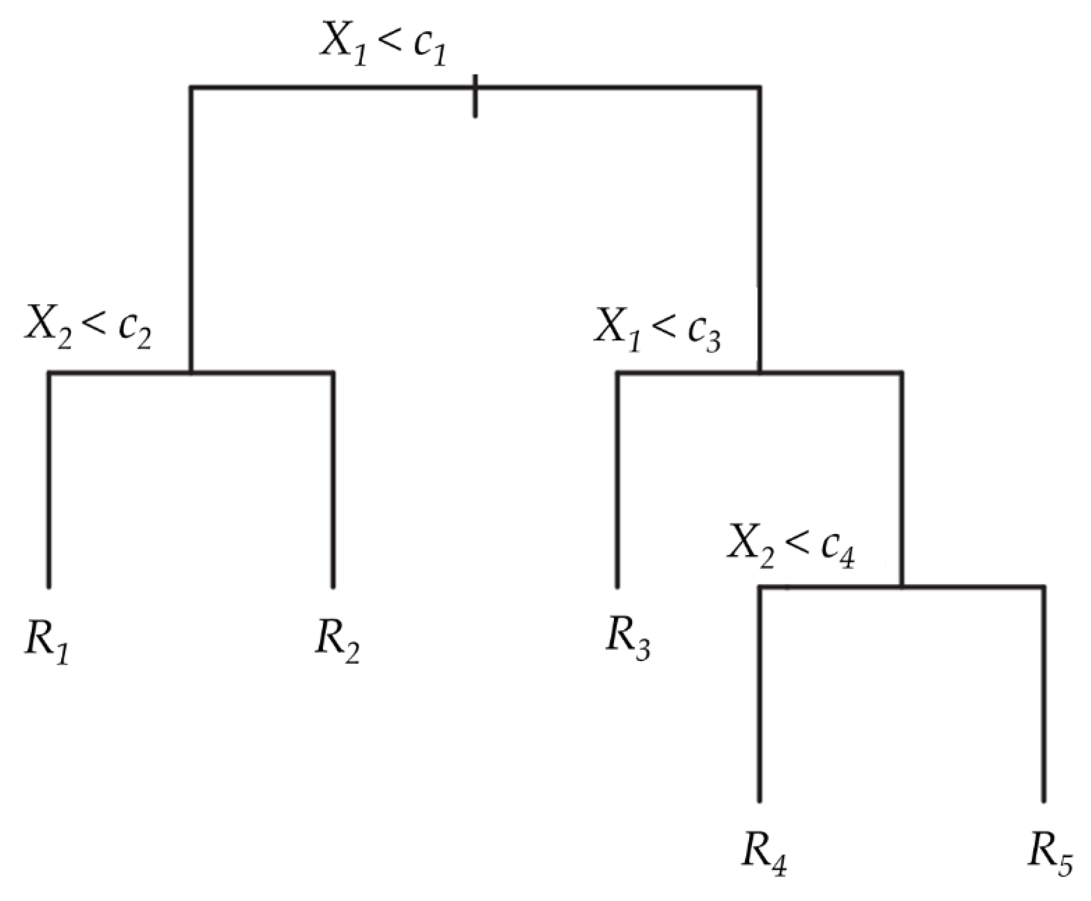
GBDT builds decision trees to explain relationships between the response (dependent variable) and predictors (independent variables). Figure 2 shows an example of a single decision tree with a response Y and two predictors, X1 and X2. All observations are first classified into two subsets based on whether X1 is bigger than c1. The subsets are further partitioned into two or more regions according to some rules, such as whether X2 is smaller than c2 or whether X1 is bigger than c3. We continue choosing the predictor and split-point for each classification until the sample in subsets is too small to split. In Figure 2, the sample is finally split into five regions (R1, R2, R3, R4, R5) using four nodes (c1, c2, c3, c4). The predicted output Fm(x) is modeled by the mean of Y in each region for continuous response and is modeled by the most frequent response of Y in the region for the discrete response. Because the classification rule does not have to be linear, decision-tree-based modeling can fit any irregular nonlinear and threshold effects.
The predictive power of any one decision tree might be limited, so an iteration process based on the gradient descent direction is used to update Fm(x). The updated model is shown below:
F m + 1 ( x ) = F m ( x ) + j = 1 J γ j m I ( x R j m )
Here Rjm refers to regions partitioned by a decision tree Fm(x), I(xRjm) equals 1 if x falls into Rjm and 0 otherwise. J is the number of regions partitioned by a decision tree, and γjm is the value of optimal gradient for the region Rjm, which could minimize the loss function L(y,Fm(x)). γjm and L(y,Fm(x)) is given as follows:
L ( y , F m ( x ) ) = l o g { 1 + e x p [ 2 y F m ( x ) ] }
when the response is dichotomous Equation (3)
L ( y , F m ( x ) ) = [ F m ( x ) y ] 2
when the response is continuous Equation (4)
γ j m = a r g m i n γ x R j m L [ y , F m ( x ) ]
The iteration process continues until cross-validation error is minimized. To address the overfitting problem, learning rate ξ is incorporated as weights into the iteration as follows:
F m + 1 ( x ) = F m ( x ) + ξ j = 1 J γ j m I ( x R j m )
With these results, the relative contribution of each independent variable is quantified as the sum of improvement in the loss function by making the split based on the variable xi. It can be described as follows:
I x i = 1 M m = 1 M I x i 2 ( T m )
I x i 2 ( T m ) = j = 1 K 1 d j ( s p l i t   a t   n o d e   j   i s   o n   v a r i a b l e s x i )
where K is the number of split points, and dj is the reduction in loss function when predictor xi is used as the splitting variable. The relative contribution of all predictors adds up to 100%.
GBDT can produce a partial dependence plot to visualize the nonlinear relationship of xs by computing the response value over the distribution of other predictors xc. It gives us a direct depiction of the predicted value of dependent variables after accounting for the effects of all other variables. Using this plot, we can specify the impact threshold beyond which proximity to the bus stop ceases to boost transit usage or reduce carbon emissions. The partial dependence of F(x) on xs can be formulated as follows:
F ¯ s ( x s ) = 1 N i = 1 N [ F ( x s , x i c ) ]
F ( x s ) = E x c [ F ( x s , x c ) ]
In this study, a five-fold cross-validation is used to build the model. The learning rate is set to 0.1. The maximum depth of each decision tree, the minimum number of terminal nodes, and the number of additive trees are set at 5, 10, and 1000, respectively, which reflects the complexity of the tree. All the parameters are within the range suggested in previous studies [30,38].

4. Results

GBDT is performed using the generalized boosted regression modeling (gbm) R package to analyze transit use and carbon emissions in central cities and suburban areas. Section 4.1 compares the performance of GBDT and traditional regression models. Section 4.2 presents the relative importance of these results, and Section 4.3 shows the nonlinear impact of bus stop proximity. Due to space limitations, the effects of other built environment factors are described in Appendix A. Section 4.4 assesses the coverage rate, with a different impact boundary drawn from the threshold effects in Section 4.3.

4.1. Performance of the GBDT Model

Table 3 shows the pseudo R2 of GBDT, which refers to the fraction of variation explained by the model and is a commonly-used evaluation criterion of predictive power [50,52,53]. As a comparison, we developed traditional regression models using the same set of variables as the GBDT model. Specifically, binomial logit is applied to model transit use, and an ordinary least squares (OLS) model is utilized to analyze carbon emissions.
The pseudo R2 for traditional models on transit use is set at 0.035, much lower than the performance for GBDT models. The low predictive power of logit regression could be attributed to the excessive amount of zero observations in the transit use models (98%), which, at worst, leads to multi-collinearity and incorrect inference [54,55]. On the contrary, GBDT models demonstrate outstanding explanatory power with imperfect data [38]. Although some sophisticated regression models can be further used to address the problem of zero inflation, the predefined model specification tends to be restrictive and burdensome [9]. The application of GBDT instead of OLS to model carbon emissions in the city center can improve the pseudo R2 from 0.133 to 0.411, which is quite similar to studies in other metropolitan areas [41]. Even when the independent variables collectively have inadequate predictability of carbon emissions in suburban areas, GBDT models still perform much better.

4.2. Relative Importance of Independent Variables

Table 4 presents the relative importance of all independent variables in predicting transit use and carbon emissions. The sum of the relative importance of all independent variables adds up to 100%, with the derived ranking based on relative importance. Table 4 illustrates that all built environment characteristics play an important role, but the ranking varies across four models, which reflects the necessity of comparative analysis.
A comparison of the central city model and the suburban model produces several interesting results. On the one hand, bus stop proximity has a larger relative contribution to transit use in suburban areas. It is the most important predictor of suburban transit use, with a relative contribution of approximately 18.14%, which exceeds the sum of demographics. In the central city, bus stop proximity ranks third, with a relative contribution of 14.51%. On the other hand, bus stop proximity in both the central city and suburban areas is important in predicting carbon emissions, showing a similar relative contribution in each. This result is acceptable; the transit supply in suburban areas is not as extensive as in the central city. A shorter distance to a bus stop can reduce transit traveling costs to a larger extent. Carbon emissions are the aggregated consequence of several behaviors, reflecting human life and footprints. Therefore, bus stop proximity describes the importance of transit service to suburban living. However, construction in Chinese suburban areas is more driving-directed [56]. Individuals there generally prefer a driving-intensive lifestyle, with longer commute distances and increased car ownership, offsetting the importance of bus stop proximity to transit use. For that reason, the contribution of bus stop proximity to carbon emissions shows no obvious difference between the central city and the suburbs, hence the ranking.
A comparison between the transit use model and the carbon emission model also generates interesting findings. Bus stop proximity is more important to transit use than to carbon emissions. In the central city, the relative contribution of bus stop proximity to transit use is 4.92 points higher than its contribution to carbon emissions. In suburban areas, it is nearly 10 points higher. The difference in importance is similar to previous findings in developing cities [57]. If travel behaviors, except for transit use, are less influenced by bus stop proximity, the combined contribution to carbon emission might not be high. Studies indicate that the relative contribution of bus stop proximity on car ownership is the lowest among built environment features [38].
Additionally, the relative importance of bus stop proximity in reducing carbon emissions is much smaller than that of developed cities. For example, in America’s Twin Cities and Guangzhou, China, proximity to transit is one of three variables with the largest predictive power [40,41], but this is not the case in Zhongshan. The difference can be ascribed to the fact that transit service is generally low-quality and inefficient in developing cities and cannot exert significant influence on nearby land use and lifestyle. Travel behaviors and carbon emissions are affected to a much lesser extent in developing cities [58].
Demographics show more similarities than differences. Generally, demographics are of relatively minor importance, whereas the total contribution of five related variables in this study is around 30%. However, it is notable that the relative importance of commuters’ education level to carbon emissions is the largest, whether in suburban areas or the city center. This association is consistent with previous studies [41] and might contribute due to two reasons. First, the relative contribution of education level to car ownership and transit use is rather large [28,39]. Second, education level plays an important role in determining in which sector people work. Highly educated people are more likely to work tertiary-sector jobs, which are more specialized than secondary-sector jobs. The tertiary-sector workers usually need to search over a larger area to find suitable employment [59], which results in longer commuting distances as well as higher carbon emissions. Given that the relative contribution of income to carbon emissions in Table 4 is quite small, the latter reason becomes more crucial.

4.3. Nonlinear and Threshold Effects

Previous studies obtained a recommended value for urban planning based on analyzing transit proximity effects on a single policy variable. Figure 3 illustrates the partial dependence plot of bus stop proximity on transit use and carbon emissions, implying that different thresholds exist and previous studies need upgrading. To avoid an overly large horizontal span impeding the investigation of the curve’s detail, bus stop proximity is narrowed to a range of 5 to 1000 m. In total, 98% of the valid commute-to-work sample data are covered by this range. Specifically, 99.5% of the central city and 97% of the suburban sample are covered. The red curve is the relationship between bus stop proximity and the dependent variables. The shadow is a 95% confidence interval, and the blue line is the smooth line.
Comparing the vertical range between the city center model and the suburban model indicates the extent to which proximity to bus stops can affect the policy variables in the city center and suburban areas, respectively. Once other variables are controlled, the range of expected transit use is 0.135–0.145 in the city center, while the range is 0.07–0.095 in suburban areas. The larger span in the suburban model (0.025) implies that bus stop proximity can increase the probability of transit use in suburban areas by a greater percentage. This result is consistent with the important comparison in Section 4.2 that reveals bus stop proximity contributes more to the variation of transit use in suburban areas (18.14%) than in the city center (14.52%). As for carbon emissions, with other factors controlled, the interval is 0.25–0.325 in the central city and 0.178–0.193 in the suburban area. Therefore, bus stop proximity can limit carbon emissions in the central city to a larger extent (0.075). This conclusion is also consistent with findings in Section 4.2, in which bus stop proximity explains the carbon emissions more in the city center (9.6%) than in the suburban areas (8.19%).
Changing patterns vary greatly among models interpreting different policy variables and different areas. In the central city, the probability of taking transit to commute is high when the distance to the bus stop is low. Once that distance exceeds 300 m, the probability of choosing bus transit decreases slowly. Then, once the distance reaches 500 m, transit use remains at a low level. As for carbon emissions in the central city, emissions remain low until the distance to the bus stop reaches 500 m. Carbon emissions steadily rise when the distance to the stop exceeds the impact boundary. In suburban areas, transit use steeply declines to a low level once the proximity to the bus stop falls outside 300 m. The carbon emissions in suburban areas tend to be low when the commuter lives near the bus stop. However, after the distance to the bus stop passes 400 m, carbon emissions initially rise dramatically and then gradually continue to rise to the highest level. The nonlinear effect pattern of bus stop proximity is much sharper in suburban areas, which is consistent with the literature on a larger impact coefficient of transit proximity outside urban districts [57]. The pattern also echoes Schwanen et al.’s work [60] by showing suburban citizens have less tolerance towards walking to a bus stop.
Based on the changing patterns, impact thresholds where the marginal effect either increases or decreases dramatically could be recognized. According to the transit use model in the city center, 300 m and 500 m can both be identified as thresholds. The marginal effect steeply declines from zero at 300 m and rapidly rises at 500 m. Nevertheless, because the probability of commuting via transit drops noticeably when the distance to a bus stop reaches 300 m, it is more proper to determine the lower threshold (300 m) as the impact boundary of a bus stop on transit use. For example, the distance from a commuter’s house to the nearest bus stop is 400 m, which is between the lower threshold and the upper threshold. However, the chance of taking public transit for this commuter is much lower than his counterparts living 300 m from the bus stop. The bus stop’s proximity is less effective in promoting transit use when the distance is beyond the lower threshold yet below the upper threshold. Similarly, 300 m and 400 m can be identified as the thresholds in the suburban transit use model, although it is also suggested to use 300 m as the impact boundary of a bus stop. As for carbon emissions, 500 m can be recognized as the only threshold in the city center model. In the suburban model, 400 m and 800 m can be viewed as the lower and upper thresholds, respectively. However, it is more appropriate to consider 400 m as the impact boundary because carbon emissions are not efficiently suppressed when the distance to the bus stop exceeds 400 m.
Further, this study summarizes the impact boundary for different policy purposes. For instance, when the planning purpose of carbon emission reduction is wanted, the distance to a bus stop for suburban individuals should be shorter than 400 m. Otherwise, the bus stop proximity could not effectively reduce carbon emissions from the journey to work. Similarly, when the policy purpose of congestion relief is proposed, the bus stop proximity is most effective below 300 m in suburban areas. Since the probability of commuting by transit in the central city declines slowly as the distance to a bus stop increases, the impact boundary can be relaxed from 300 to 400 m. Table 5 summarizes the recommended values of bus stop radius for different policy purposes in different areas, which are much lower and stricter than that in developed cities [61].
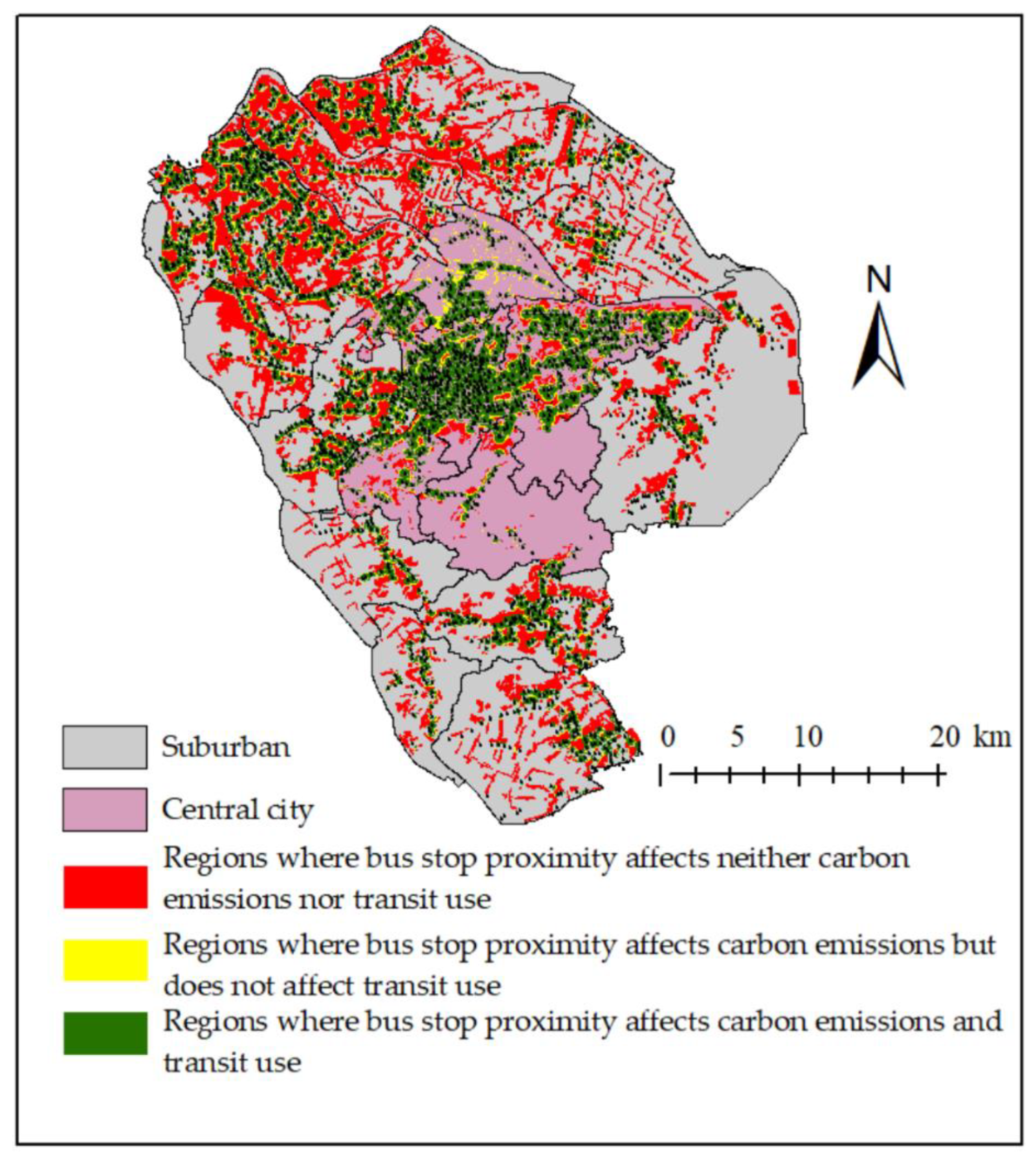
The above impact boundary can be utilized as the basis to quantify the extent to which regional development is impacted by the transit system. As depicted in Figure 4, the red areas are too far from the bus stop to be influenced, while the green areas are proximate enough to the stop. Consequently, bus stop proximity is conducive to transit promotion and carbon mitigation in green areas but not red areas. As for the built-up areas in yellow, their distance to the bus stop is too far to increase transit use but is close enough to reduce carbon emissions. Therefore, current transit construction is effective for carbon reduction but trivial to congestion relief in those yellow regions. Figure 4 suggests that the presence of bus transit has a limited impact on daily suburban life. The spatial heterogeneity is congruent with the literature on poor transit provision and reflects an urgent need for preferential transit improvement in suburban areas [11,58].

4.4. The Stop Coverage Rate

The threshold of proximity impact can be applied to determine an appropriate buffer around bus stops, which guarantees the validity of the land use performance assessment. If the land use pattern is evaluated for the sake of transit development and congestion relief, it is suggested to measure the percent coverage of the built-up area by bus stops with a radius of 300 m and 400 m in the suburban regions and the central city, respectively. Assessment of 500-m bus stop coverage does not accurately capture the land use performance on increasing transit use [4,41].
This section uses the impact boundary described in Table 5 to calculate how many populations and areas have appropriate proximity to bus stops upon consideration of different policy purposes. The population in the travel survey and built-up areas are summarized within the given threshold and then further divided by the total observations and the total built-up areas to obtain the coverage rate around the stops. Additionally, according to the Standard for Urban Comprehensive Transport System Planning issued by the Ministry of Housing and Urban-Rural Development in 2018 [62] and the System of Assessment Indicators for Transit Metropolis issued by the Ministry of Transport in 2013 [63], 500-m bus stop coverage is one of the important guidelines for city development. Therefore, the bus service coverage rate based on national criteria in the planning code is also computed as a comparison. The coverage rate is presented in Table 6.
When the focus is on promoting transit use, 87.1% of commuters and 71.4% of the built area in the central city have appropriate proximity to a bus stop. However, only 57.4% of commuters and 44.9% of built suburban areas enjoy sufficient accessibility to bus transit service. On the other hand, if the reduction in carbon emissions is prioritized, 93.8% of commuters and 83.3% of the built area in the central city are located in a bus stop catchment area. Meanwhile, 74% of commuters and 61.5% of built suburban areas are covered by the bus transit system.
The impact boundary and related criteria for different policy purposes influence the performance assessment results of land use patterns. Assessed under the current national criterion, which defines a 500-m station buffer, the coverage rate of the population in the central city and suburban areas is as much as 90% and 80%, respectively; the coverage rate of the built area is as much as 80% and 70%, respectively. If the land use pattern is assessed to reduce carbon emissions, the coverage rate is less satisfactory. When the stricter criterion for congestion relief is adopted, the coverage rate is far from efficient. More than half of built suburban areas lack appropriate access to a bus stop. An imbalance exists between the central city and suburban areas, which is consistent with previous studies [58].

5. Discussion and Conclusions

This study utilizes the GBDT model to examine the nonlinear and threshold effects of bus stop proximity and its impact on different policy purposes. The GBDT model demonstrates a stronger predictive power than traditional regressions, which is the most important advantage of the method used in this study. Two essential conclusions can be drawn. First, the association between transit proximity and carbon emissions in Zhongshan is weaker than that found in developed cities [41]. In developing cities similar to Zhongshan, the relative importance of transit proximity, as it influences carbon emissions, is lower than it affects transit use. Both phenomena might originate from the diminished ability of bus transit services in developing cities to strongly influence urban residents’ lifestyles [58]. Second, the effects of bus stop proximity in the central city extend to 500 m on carbon emissions but only to 400 m on transit use. The impact boundary in suburban areas is 400 m for carbon emissions but 300 m for transit use. The varied threshold affects the standard validity for land use assessments to realize different policy goals. When the bus stop coverage rate is employed to evaluate land use patterns, its performance in promoting commuting by transit is far from efficient, while the valuation based on the policy goal of emission reduction is still good. The assessment based on the present national standard overestimates the efficiency of land use patterns, with a massive regional imbalance. The divergence of assessment implies that current land use patterns perform well in reducing carbon emissions but terribly in congestion relief [4].
The contribution made by this study to the existing literature is twofold. First, this study investigates the nonlinear effects of bus stop proximity in developing cities and illustrates that the recommendations for urban planning in developed cities are not perfectly transferable to developing cities [38,61]. Second, this study compares the threshold effects on different policy variables and finds that bus stop proximity effects extend to diverse ranges within different policy contexts [41]. The variation in impact thresholds implies that proper standards should be adopted for land use planning to best support multiple aims.
These findings have practical implications. First, enhancing the coverage rate of bus stops is one indicator proposed by the central government to regulate urban development and measure transit accessibility at the city level. We suggest that the station coverage rate should be calculated on a different basis in different cities. Developing and small-to-medium cities should use a smaller boundary to calculate the coverage rate so that the assessment can accurately reflect the validity of land use and designate areas requiring improvement. Otherwise, the assessment might overestimate land use performance.
Second, this study argues for adopting appropriate standards to assess urban land use rather than requiring local governments to increase the coverage rate during urban development processes. Increasing the 300-m bus stop coverage rate is costly. Instead, we suggest alternative policies. For example, supportive measures can be adopted by providing public bicycles to reduce the negative impact of commuters’ long distances to their nearest bus stop. The quality of bus service can also be enhanced by signal control measures to enlarge the catchment area and the impact boundary of proximity to transit [64,65]. Finally, city managers can focus more on the station coverage rate of the population rather than that of the built area by prioritizing better bus service around densely populated areas.
Third, because urban planning and developments usually have many targets, land use indicators should address consistency across multiple policy goals. The gains of social benefits from multiple dimensions have to be carefully balanced when designing the national transit metropolis initiative. The policy goals in this study can still be coordinated to some extent. It is more important to recommend an effective range for land use when goals of greater disparity exist. This also applies to other built environment features and is not limited to bus stop proximity. For instance, although high density can facilitate transit use and urban vitality [45,66], it can also reduce citizens’ well-being [67,68]. A comparative analysis of threshold effects for different policy purposes would be especially helpful in deriving a proper recommendation indicator for urban planning.
Therefore, this study may provide inspiration for future research on investigating land use management to better coordinate multiple policy goals. For example, future studies could elucidate how land use patterns effectively meet the demands of different social groups. For instance, developing the city as both elder-friendly and child-friendly is difficult but essential to ensure transportation equity. In addition, future studies could analyze how travel demand management affects the effective range of each constructed environmental feature. It would be helpful to consider policies facilitating multidimensional sustainability.
This study does have several limitations. Restricted by the travel survey data, the carbon emission factors are based on existing works that do not consider vehicle type or occupancy. This study applies the GBDT model, which is not able to uncover the pathway of bus proximity effects on carbon emissions. Lastly, the relationship in this study is found to be relevant rather than causal.

Author Contributions

Conceptualization, Z.H. and Y.P.; methodology, Z.H. and Y.P.; software, Z.H.; validation, Z.H. and Y.P.; formal analysis, Z.H. and Y.P.; investigation, Z.H. and Y.P.; resources, Z.H. and Y.P.; data curation, Z.H. and Y.P.; writing—original draft preparation, Z.H. and Y.P.; writing—review and editing, Z.H. and Y.P.; visualization, Z.H. and Y.P.; supervision, Y.P.; project administration, Z.H. and Y.P. All authors have read and agreed to the published version of the manuscript.

Funding

This research was funded by the Shenzhen Municipal Natural Science Foundation (GXWD20201231165807007-20200811151825001).

Data Availability Statement

Not applicable.

Conflicts of Interest

The authors declare no conflict of interest.

Appendix A

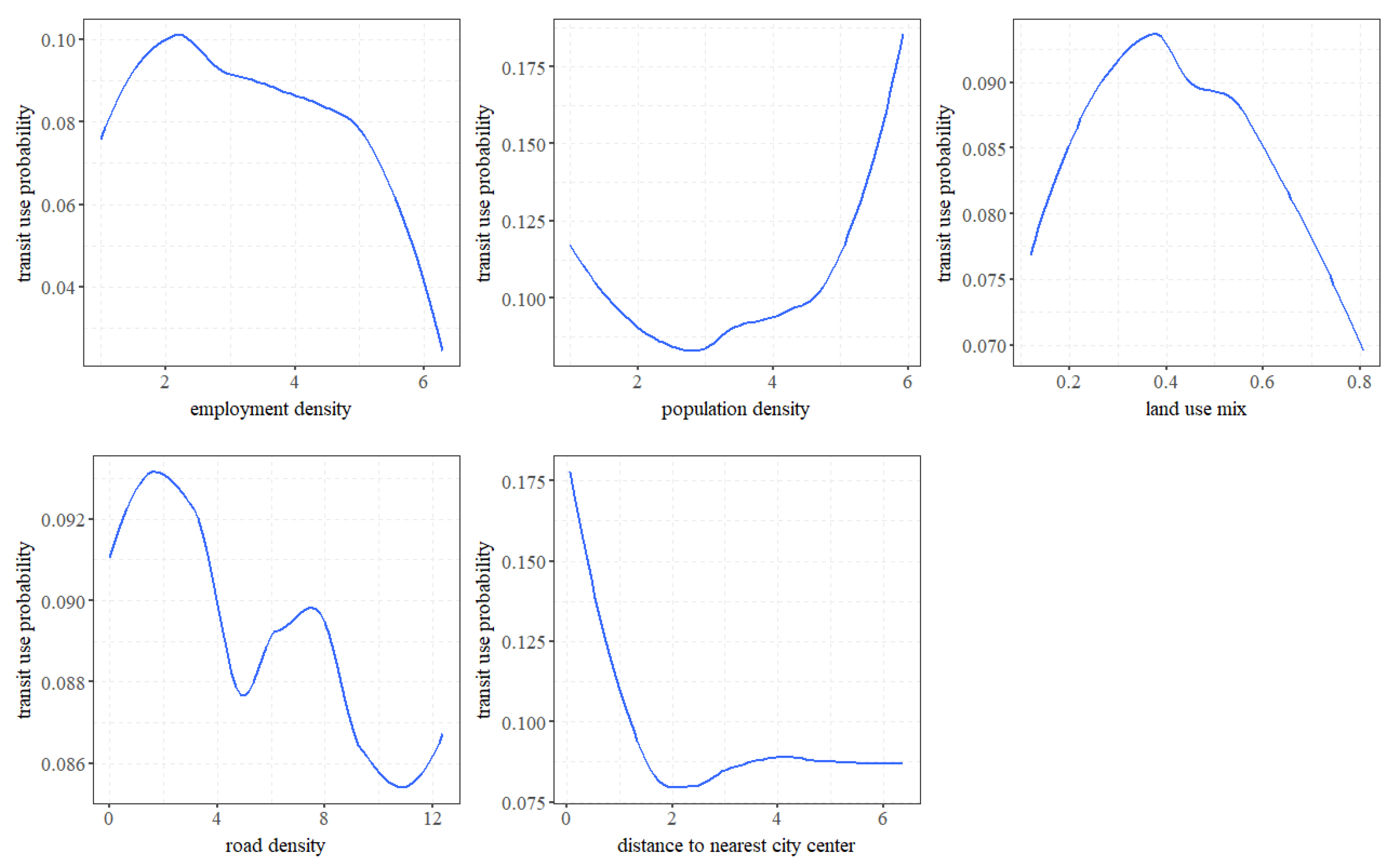
The appendix illustrates the nonlinear effects of other built environment features, including employment density, population density, land use mix, road density, and distance to the nearest city center.
Figure A1 and Figure A2 suggest that a slight increase in employment density can increase the transit commuting probability, as inner urban areas often have inadequate parking supply for workers [69]. However, as the employment density increases, the congestion impact outweighs the parking impact, and transit use declines [70]. The relationship between population density and transit is a U-shaped curve. Only when the population density is high enough to support the transit construction can it facilitate transit use [71].
Road density in the central city can improve street connectivity and increase the probability of using transit. However, because the transit supply in suburban areas is poor [58], the higher road density elevates car driving over transit use, which decreases. The land use mix in the central city promotes transit use, whereas too high or too low entropy in suburban areas suppresses transit use. To show the detailed pattern, the distance to the neatest city center is narrowed to a range with 99% of the sample included. In the central city, as a commuter’s location moves farther from the nearest city center, transit use decreases. However, when the distance to the nearest city center exceeds a certain threshold, the commuter is affected by another city center, and transit use rises [38]. In suburban areas, in contrast, the transit commuting probability continues to decrease as the distance to the nearest city center increases.
Figure A1. Nonlinear effects of other built environment features on transit use in the central city.
Land 12 00028 g0a1
Figure A2. Nonlinear effects of other built environment features on transit use in suburban areas.
Land 12 00028 g0a2
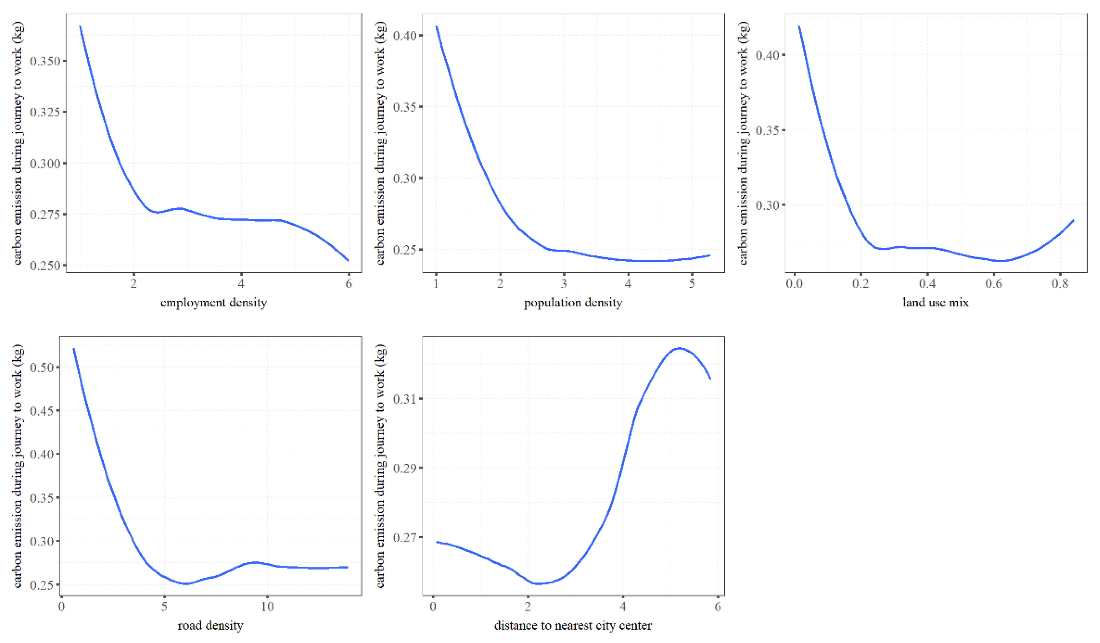
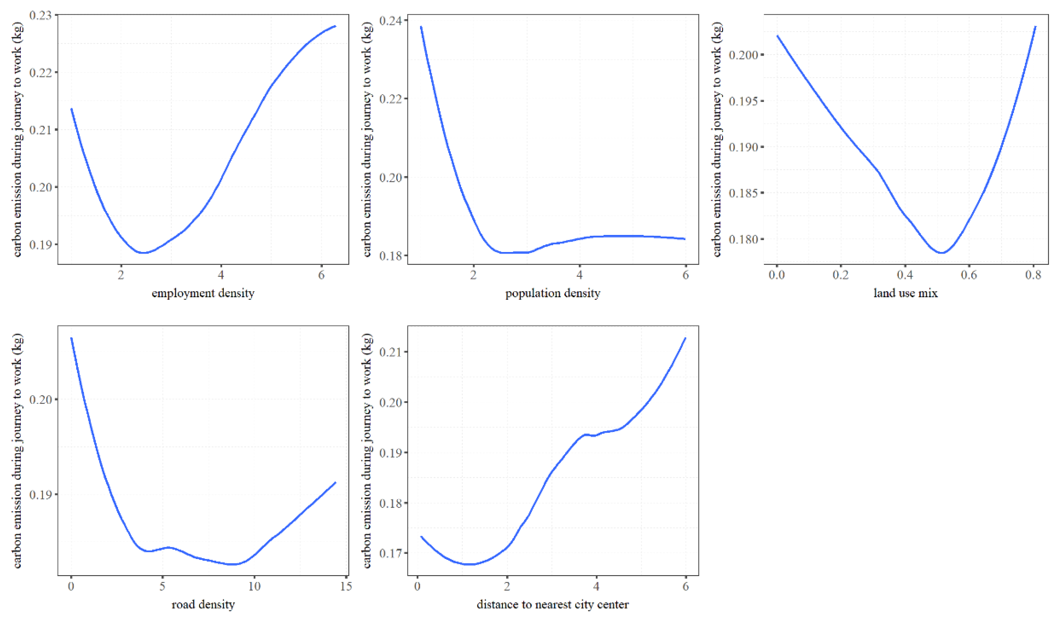
Figure A3 and Figure A4 illustrate that population density has a negative relationship with carbon emissions because higher density can facilitate transit use and reduce trip distance [30,71]. A medium-degree mixture of land use helps to minimize commuting-related carbon emissions. When road density increases from the lowest value to 10, carbon emissions fall. When road density exceeds 10 in suburban areas, the shortage of transit supply induces car driving and carbon emissions to increase [58]. Within a 2 km radius of a city center, carbon emissions remain at a low level. However, when the distance to the city center continues to increase beyond the threshold, transit supply decreases, vehicle ownership increases, and commuting distance increases [38,41]. Carbon emissions as the combined outcome of these factors also rise.
In the central city, population density has a negative influence on carbon emissions, while its effects weaken outside the impact boundary as a consequence of congestion. In suburban areas, population density exerts a positive influence on carbon emissions after the threshold is reached. For 80% of suburban observations, population density is lower than three, and the increase in population density does help to reduce carbon emissions. For the other 20% of suburban observations, residents mostly reside in industrial parks of singular land use. The higher the population density, the larger the scale of an industrial park; this leads to longer trip distances, which decrease transit use and thereby increase carbon emissions.
Figure A3. Nonlinear effects of other built environment features on carbon emissions in the central city.
Land 12 00028 g0a3
Figure A4. Nonlinear effects of other built environment features on carbon emissions in suburban areas.
Land 12 00028 g0a4

References

  1. Zuo, T.; Wei, H.; Chen, N. Promote transit via hardening first-and-last-mile accessibility: Learned from modeling commuters’ transit use. Transp. Res. Part D Transp. Environ. 2020, 86, 102446. [Google Scholar] [CrossRef]
  2. Gim, T.H.T. Analyzing the city-level effects of land use on travel time and CO2 emissions: A global mediation study of travel time. Int. J. Sustain. Transp. 2022, 16, 496–513. [Google Scholar] [CrossRef]
  3. Ewing, R.; Cervero, R. Travel and the built environment. J. Am. Plan. Assoc. 2010, 76, 265–294. [Google Scholar] [CrossRef]
  4. Park, K.; Ewing, R.; Sabouri, S.; Choi, D.; Hamidi, S.; Tian, G. Guidelines for a Polycentric Region to Reduce Vehicle Use and Increase Walking and Transit Use. J. Am. Plan. Assoc. 2020, 86, 236–249. [Google Scholar] [CrossRef]
  5. Yu, L.; Xie, B.; Chan, E.H.W. Exploring impacts of the built environment on transit travel: Distance, time and mode choice, for urban villages in Shenzhen, China. Transp. Res. Part E Logist. Transp. Rev. 2019, 132, 57–71. [Google Scholar] [CrossRef]
  6. Ma, J.; Liu, Z.; Chai, Y. The impact of urban form on CO2 emission from work and non-work trips: The case of Beijing, China. Habitat Int. 2015, 47, 1–10. [Google Scholar] [CrossRef]
  7. Sam Zimbabwe, E.G.; APTA. Defining Transit Areas of Influence; APTA Standards Development Program; American Public Transportation Association: Washington, DC, USA, 2009; p. 11. [Google Scholar]
  8. Le, J.; Ye, K. Measuring City-Level Transit Accessibility Based on the Weight of Residential Land Area: A Case of Nanning City, China. Land 2022, 11, 1468. [Google Scholar] [CrossRef]
  9. Yang, J.; Su, P.; Cao, J. On the importance of Shenzhen metro transit to land development and threshold effect. Transp. Policy 2020, 99, 1–11. [Google Scholar] [CrossRef]
  10. Galster, G.C. Nonlinear and Threshold Effects Related to Neighborhood: Implications for Planning and Policy. J. Plan. Lit. 2018, 33, 492–508. [Google Scholar] [CrossRef]
  11. Mwale, M.; Luke, R.; Pisa, N. Factors that affect travel behaviour in developing cities: A methodological review. Transp. Res. Interdiscip. Perspect. 2022, 16, 100683. [Google Scholar] [CrossRef]
  12. Tao, T.; Wang, J.; Cao, X. Exploring the non-linear associations between spatial attributes and walking distance to transit. J. Transp. Geogr. 2020, 82, 102560. [Google Scholar] [CrossRef]
  13. Guan, C.H.; Song, J.; Keith, M.; Akiyama, Y.; Shibasaki, R.; Sato, T. Delineating urban park catchment areas using mobile phone data: A case study of Tokyo. Comput. Environ. Urban Syst. 2020, 81, 101474. [Google Scholar] [CrossRef]
  14. Zhang, M. The role of land use in travel mode choice: Evidence from Boston and Hong Kong. J. Am. Plan. Assoc. 2004, 70, 344–360. [Google Scholar] [CrossRef]
  15. Shen, Q.; Chen, P.; Pan, H. Factors affecting car ownership and mode choice in rail transit-supported suburbs of a large Chinese city. Transp. Res. Part A Policy Pract. 2016, 94, 31–44. [Google Scholar] [CrossRef]
  16. Ao, Y.; Zhang, Y.; Wang, Y.; Chen, Y.; Yang, L. Influences of rural built environment on travel mode choice of rural residents: The case of rural Sichuan. J. Transp. Geogr. 2020, 85, 102708. [Google Scholar] [CrossRef]
  17. Zhao, P. The Impact of the Built Environment on Individual Workers’ Commuting Behavior in Beijing. Int. J. Sustain. Transp. 2013, 7, 389–415. [Google Scholar] [CrossRef]
  18. Ha, J.; Lee, S.; Ko, J. Unraveling the impact of travel time, cost, and transit burdens on commute mode choice for different income and age groups. Transp. Res. Part A Policy Pract. 2020, 141, 147–166. [Google Scholar] [CrossRef]
  19. Crotti, D.; Grechi, D.; Maggi, E. Proximity to public transportation and sustainable commuting to college. A case study of an Italian suburban campus. Case Stud. Transp. Policy 2022, 10, 218–226. [Google Scholar] [CrossRef]
  20. Kim, H.; Nam, J. The size of the station influence area in Seoul, Korea: Based on the survey of users of seven stations. Int. J. Urban Sci. 2013, 17, 331–349. [Google Scholar] [CrossRef]
  21. Alshalalfah, B.W.; Shalaby, A.S. Case Study: Relationship of Walk Access Distance to Transit with Service, Travel, and Personal Characteristics. J. Urban Plan. Dev. 2007, 133, 114–118. [Google Scholar] [CrossRef]
  22. Torres, M.A.; Oh, H.W.; Lee, J. The Built Environment and Children’s Active Commuting to School: A Case Study of San Pedro De Macoris, the Dominican Republic. Land 2022, 11, 1454. [Google Scholar] [CrossRef]
  23. Ding, C.; Cao, X.; Wang, Y. Synergistic effects of the built environment and commuting programs on commute mode choice. Transp. Res. Part A Policy Pract. 2018, 118, 104–118. [Google Scholar] [CrossRef]
  24. Viggiano, C.; Koutsopoulos, H.N.; Attanucci, J.; Wilson, N.H.M. Inferring public transport access distance from smart card registration and transaction data. Transp. Res. Rec. 2016, 2544, 55–62. [Google Scholar] [CrossRef]
  25. Guan, X.; Wang, D.; Jason Cao, X. The role of residential self-selection in land use-travel research: A review of recent findings. Transp. Rev. 2020, 40, 267–287. [Google Scholar] [CrossRef]
  26. Cao, X.; Xu, Z.; Fan, Y. Exploring the connections among residential location, self-selection, and driving: Propensity score matching with multiple treatments. Transp. Res. Part A Policy Pract. 2010, 44, 797–805. [Google Scholar] [CrossRef]
  27. Guerra, E.; Cervero, R.; Tischler, D. Half-mile circle: Does it best represent transit station catchments? Transp. Res. Rec. 2012, 2276, 101–109. [Google Scholar] [CrossRef] [Green Version]
  28. Ding, C.; Liu, T.; Cao, X.; Tian, L. Illustrating nonlinear effects of built environment attributes on housing renters ’ transit commuting. Transp. Res. Part D 2022, 112, 103503. [Google Scholar] [CrossRef]
  29. Cao, X.; Næss, P.; Wolday, F. Examining the effects of the built environment on auto ownership in two Norwegian urban regions. Transp. Res. Part D Transp. Environ. 2019, 67, 464–474. [Google Scholar]
  30. Ding, C.; Cao, X.; Næss, P. Applying gradient boosting decision trees to examine non-linear effects of the built environment on driving distance in Oslo. Transp. Res. Part A Policy Pract. 2018, 110, 107–117. [Google Scholar] [CrossRef]
  31. Lee, S.; Lee, B. Comparing the impacts of local land use and urban spatial structure on household VMT and GHG emissions. J. Transp. Geogr. 2020, 84, 102694. [Google Scholar] [CrossRef]
  32. Ao, Y.; Yang, D.; Chen, C.; Wang, Y. Effects of rural built environment on travel-related CO2 emissions considering travel attitudes. Transp. Res. Part D Transp. Environ. 2019, 73, 187–204. [Google Scholar] [CrossRef]
  33. Cao, X.; Yang, W. Examining the effects of the built environment and residential self-selection on commuting trips and the related CO2 emissions: An empirical study in Guangzhou, China. Transp. Res. Part D Transp. Environ. 2017, 52, 480–494. [Google Scholar] [CrossRef]
  34. Zhu, W.; Ding, C.; Cao, X. Built environment effects on fuel consumption of driving to work: Insights from on-board diagnostics data of personal vehicles. Transp. Res. Part D Transp. Environ. 2019, 67, 565–575. [Google Scholar] [CrossRef]
  35. Wang, X.; Liu, C.; Kostyniuk, L.; Shen, Q.; Bao, S. The influence of street environments on fuel efficiency: Insights from naturalistic driving. Int. J. Environ. Sci. Technol. 2014, 11, 2291–2306. [Google Scholar] [CrossRef] [Green Version]
  36. Boarnet, M.G.; Wang, X.; Houston, D. Can New Light Rail Reduce Personal Vehicle Carbon Emissions? a Before-After, Experimental-Control Evaluation in Los Angeles. J. Reg. Sci. 2017, 57, 523–539. [Google Scholar] [CrossRef]
  37. Gao, J.; Ma, S.; Li, L.; Zuo, J.; Du, H. Does travel closer to TOD have lower CO2 emissions? Evidence from ride-hailing in Chengdu, China. J. Environ. Manag. 2022, 308, 114636. [Google Scholar] [CrossRef] [PubMed]
  38. Shao, Q.; Zhang, W.; Jason, X.; Yang, J. Nonlinear and interaction effects of land use and motorcycles/E-bikes on car ownership. Transp. Res. Part D 2022, 102, 103115. [Google Scholar] [CrossRef]
  39. Wang, X.; Yin, C.; Zhang, J.; Shao, C.; Wang, S. Nonlinear effects of residential and workplace built environment on car dependence. J. Transp. Geogr. 2021, 96, 103207. [Google Scholar] [CrossRef]
  40. Yang, W.; Zhou, S. Using decision tree analysis to identify the determinants of residents’ CO2 emissions from different types of trips: A case study of Guangzhou, China. J. Clean. Prod. 2020, 277, 124071. [Google Scholar] [CrossRef]
  41. Wu, X.; Tao, T.; Cao, J.; Fan, Y.; Ramaswami, A. Examining threshold effects of built environment elements on travel-related carbon-dioxide emissions. Transp. Res. Part D Transp. Environ. 2019, 75, 1–12. [Google Scholar] [CrossRef]
  42. Kong, H.; Jin, S.T.; Sui, D.Z. Deciphering the relationship between bikesharing and public transit: Modal substitution, integration, and complementation. Transp. Res. Part D Transp. Environ. 2020, 85, 102392. [Google Scholar] [CrossRef]
  43. El-Geneidy, A.; Grimsrud, M.; Wasfi, R.; Tétreault, P.; Surprenant-Legault, J. New evidence on walking distances to transit stops: Identifying redundancies and gaps using variable service areas. Transportation 2014, 41, 193–210. [Google Scholar] [CrossRef]
  44. Yang, Y.; Wang, C.; Liu, W.; Zhou, P. Understanding the determinants of travel mode choice of residents and its carbon mitigation potential. Energy Policy 2018, 115, 486–493. [Google Scholar] [CrossRef]
  45. Zhang, W.; Lu, D.; Chen, Y.; Liu, C. Land use densification revisited: Nonlinear mediation relationships with car ownership and use. Transp. Res. Part D Transp. Environ. 2021, 98, 102985. [Google Scholar] [CrossRef]
  46. Zeng, J.; Qian, Y.; Mi, P.; Zhang, C.; Yin, F.; Zhu, L.; Xu, D. Freeway traffic flow cellular automata model based on mean velocity feedback. Phys. A Stat. Mech. Appl. 2021, 562, 125387. [Google Scholar] [CrossRef]
  47. Chakrabarti, S. How can public transit get people out of their cars? An analysis of transit mode choice for commute trips in Los Angeles. Transp. Policy 2017, 54, 80–89. [Google Scholar] [CrossRef]
  48. The 2006 IPCC Guidelines for National Greenhouse Gas Inventories. Available online: https://www.ipcc.ch/report/2019-refinement-to-the-2006-ipcc-guidelines-for-national-greenhouse-gas-inventories/ (accessed on 17 December 2022).
  49. Friedman, J.H. Greedy function approximation: A gradient boosting machine. Ann. Stat. 2001, 29, 1189–1232. [Google Scholar] [CrossRef]
  50. Tu, M.; Li, W.; Orfila, O.; Li, Y.; Gruyer, D. Exploring nonlinear effects of the built environment on ridesplitting: Evidence from Chengdu. Transp. Res. Part D Transp. Environ. 2021, 93, 102776. [Google Scholar] [CrossRef]
  51. Gan, L.; Ren, H.; Xiang, W.; Wu, K.; Cai, W. Nonlinear influence of public services on urban housing prices: A case study of China. Land 2021, 10, 1007. [Google Scholar] [CrossRef]
  52. Zhao, X.; Yan, X.; Yu, A.; van Hentenryck, P. Prediction and behavioral analysis of travel mode choice: A comparison of machine learning and logit models. Travel Behav. Soc. 2020, 20, 22–35. [Google Scholar] [CrossRef]
  53. Schonlau, M. Boosted regression (boosting): An introductory tutorial and a Stata plugin. Stata J. 2005, 5, 330–354. [Google Scholar] [CrossRef] [Green Version]
  54. Lambert, D. Zero-inflated poisson regression, with an application to defects in manufacturing. Technometrics 1992, 34, 1–14. [Google Scholar] [CrossRef]
  55. Cervero, R. Built environments and mode choice: Toward a normative framework. Transp. Res. Part D Transp. Environ. 2002, 7, 265–284. [Google Scholar] [CrossRef]
  56. Martin, E.W.; Shaheen, S.A. Evaluating public transit modal shift dynamics in response to bikesharing: A tale of two U.S. cities. J. Transp. Geogr. 2014, 41, 315–324. [Google Scholar] [CrossRef] [Green Version]
  57. Feng, R.; Feng, Q.; Jing, Z.; Zhang, M.; Yao, B. Association of the built environment with motor vehicle emissions in small cities. Transp. Res. Part D Transp. Environ. 2022, 107, 103313. [Google Scholar] [CrossRef]
  58. Hu, H.; Xu, J.; Shen, Q.; Shi, F.; Chen, Y. Travel mode choices in small cities of China: A case study of Changting. Transp. Res. Part D Transp. Environ. 2018, 59, 361–374. [Google Scholar] [CrossRef]
  59. Zhou, X.; Yeh, A.G.O.; Li, W.; Yue, Y. A commuting spectrum analysis of the jobs–housing balance and self-containment of employment with mobile phone location big data. Environ. Plan. B Urban Anal. City Sci. 2018, 45, 434–451. [Google Scholar] [CrossRef]
  60. Schwanen, T.; Dieleman, F.M.; Dijst, M. Travel behaviour in Dutch monocentric and policentric urban systems. J. Transp. Geogr. 2001, 9, 173–186. [Google Scholar] [CrossRef]
  61. Zhang, W.; Lu, D.; Zhao, Y.; Luo, X.; Yin, J. Incorporating polycentric development and neighborhood life-circle planning for reducing driving in Beijing: Nonlinear and threshold analysis. Cities 2021, 121, 103488. [Google Scholar] [CrossRef]
  62. Standard for Urban Comprehensive Transport System Planning. Available online: https://www.mohurd.gov.cn/gongkai/fdzdgknr/tzgg/201903/20190320_239844.html (accessed on 17 December 2022). (In Chinese)
  63. System of Assessment Indicators for Transit Metropolis. Available online: https://xxgk.mot.gov.cn/2020/jigou/ysfws/202006/t20200623_3314986.html. (accessed on 17 December 2022). (In Chinese)
  64. Qian, Y.; Zeng, J.; Wang, N.; Zhang, J.; Wang, B. A traffic flow model considering influence of car-following and its echo characteristics. Nonlinear Dyn. 2017, 89, 1099–1109. [Google Scholar] [CrossRef]
  65. Zeng, J.; Qian, Y.; Lv, Z.; Yin, F.; Zhu, L.; Zhang, Y.; Xu, D. Expressway traffic flow under the combined bottleneck of accident and on-ramp in framework of Kerner’s three-phase traffic theory. Phys. A Stat. Mech. Appl. 2021, 574, 125918. [Google Scholar] [CrossRef]
  66. Yang, J.; Cao, J.; Zhou, Y. Elaborating non-linear associations and synergies of subway access and land uses with urban vitality in Shenzhen. Transp. Res. Part A Policy Pract. 2021, 144, 74–88. [Google Scholar] [CrossRef]
  67. Cao, J.; Hao, Z.; Yang, J.; Yin, J.; Huang, X. Prioritizing neighborhood attributes to enhance neighborhood satisfaction: An impact asymmetry analysis. Cities 2020, 105, 102854. [Google Scholar] [CrossRef]
  68. Ma, Y.; Yang, Y.; Jiao, H. Exploring the impact of urban built environment on public emotions based on social media data: A case study of Wuhan. Land 2021, 10, 986. [Google Scholar] [CrossRef]
  69. Ding, C.; Cao, X.; Dong, M.; Zhang, Y.; Yang, J. Non-linear relationships between built environment characteristics and electric-bike ownership in Zhongshan, China. Transp. Res. Part D Transp. Environ. 2019, 75, 286–296. [Google Scholar] [CrossRef]
  70. Zeng, J.; Qian, Y.; Yin, F.; Zhu, L.; Xu, D. A multi-value cellular automata model for multi-lane traffic flow under lagrange coordinate. Comput. Math. Organ. Theory 2022, 28, 178–192. [Google Scholar] [CrossRef]
  71. Yao, Z.; Kim, C. The Changes of Urban Structure and Commuting: An Application to Metropolitan Statistical Areas in the United States. Int. Reg. Sci. Rev. 2019, 42, 3–30. [Google Scholar] [CrossRef]
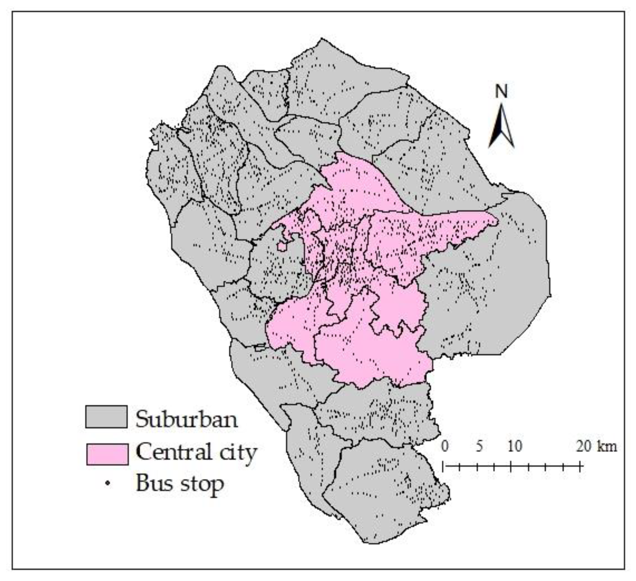
Figure 1. Study area.
Land 12 00028 g001
Figure 2. A single decision tree.
Land 12 00028 g002
Figure 3. Proximity effects on transit use and commuting-related carbon emission.
Land 12 00028 g003
Figure 4. Regions affected by bus stop proximity from different policy aspects.
Land 12 00028 g004
Table 1. Carbon emission factors for different travel modes (kg/person km).
ReferencesStudy AreaSourceWalk, BikeElectric BikeBusMotorcycleCar
Wu et al. (2019) [41]Minneapolis, USAU.S. Department of Transportation0-0.199-0.299
Yang et al. (2018) [44]Beijing, ChinaEC’s reports; Department of Energy and Climate Change in UK00.0080.035-0.126
Cao and Yang (2017) [33]Guangzhou, ChinaEntwicklungsbank0-0.026-0.233
Ao et al. (2019) [32]Sichuan, ChinaCalculation from model proposed by EC; EC’ reports; Department of Energy and Climate Change in UK00.0080.0350.04720.126
This studyZhongshan, ChinaSame as Ao et al. (2019) [32]00.0080.0350.04720.126
Table 2. Variable definitions and descriptive statistics.
NameDefinitionMin.Max.MeanSt. Dev.Source
Dependent variable
Transit useA dummy variable indicating whether respondent chose to take bus0.001.000.020.14Travel survey
Carbon emissionsCO2 emitted during the commute to work, which equals DiRi (kg)0.009.980.260.56Di from Baidu Map; Ri from Ao et al.’s work [32]
Key variable
Proximity to bus stopStraight-line distance from house centroid to the nearest bus stop (m)1.303273.45307.80253.73Location from Baidu Map; Calculation using ArcGIS
Built environment
Employment densityAverage employment density within 1-km buffer around the house (scale)1.006.292.551.05Baidu Map
Population densityAverage employment density within 1-km buffer around the house (scale)1.006.002.461.00Baidu Map
Land use mixLand use entropy0.000.840.490.14Land use data
Road densityStreet length per km2 within 1-km buffer around the house (km/km2)0.0014.456.632.88Land use data
Distance to the nearest city centerStraight-line distance from house centroid to nearest city center (km)0.069.472.581.56Land use data
Demographics
GenderA dummy variable indicating whether respondent is female0.001.000.560.50Travel survey
IncomeLevel of respondent’s annual income: <50,000 noted as 0, 50–100,000 as 1, 100–200,000 as 2, >200,000 as 30.003.001.470.78Travel survey
EducationLevel of respondent’s education: primary school noted as 0, junior high school as 1, senior high school as 2, vocational education as 3, bachelor and higher as 40.004.002.101.11Travel survey
Family sizeNumber of people in respondent’s family1.0011.003.281.32Travel survey
Number of childrenNumber of respondent’s children0.005.000.390.63Travel survey
Table 3. Performance comparison of R2 for GBDT and traditional regression models.
AreaDependent VariablesGBDTTraditional Regression Model
Central cityTransit use0.3510.035
Carbon emissions0.4110.133
Suburban areasTransit use0.6130.035
Carbon emissions0.1920.067
Table 4. Relative importance of independent variables on transit use and carbon emissions.
PredictorCentral CitySuburban Areas
Transit UseCarbon EmissionsTransit UseCarbon Emissions
Relative Importance (%)RankingRelative Importance (%)RankingRelative Importance (%)RankingRelative Importance (%)Ranking
Proximity to bus stop14.5239.60618.1418.197
Employment density15.82111.48413.3539.545
Population density12.15613.01311.5969.156
Land use mix13.70510.24512.35411.493
Road density14.6725.84811.67511.384
Distance to the nearest city center14.48414.18217.09212.722
Gender3.4195.6993.4595.668
Income2.11107.8071.37115.389
Education4.49715.3514.13819.941
Family size3.6685.51104.4474.4810
Number of children0.98111.29112.44102.0711
Table 5. Impact boundary of bus stops.
Suggested Level (m)
Central CitySuburban Areas
Policy purpose
Promote transit use400300
Reduce carbon emission500400
Table 6. Bus stop coverage under different criteria.
Coverage Rate of Population (%)Coverage Rate of Built Area (%)
Central CitySuburban AreasCentral CitySuburban Areas
Policy purpose of criteria
Current national criteria (500 m)93.883.883.373.5
Promote transit use87.157.471.444.9
Reduce carbon emissions93.874.083.361.5
Disclaimer/Publisher’s Note: The statements, opinions and data contained in all publications are solely those of the individual author(s) and contributor(s) and not of MDPI and/or the editor(s). MDPI and/or the editor(s) disclaim responsibility for any injury to people or property resulting from any ideas, methods, instructions or products referred to in the content.