
Comparing Nonlinear and Threshold Effects of Bus Stop Proximity on Transit Use and Carbon Emissions in Developing Cities


Abstract
:1. Introduction
2. Literature Review
3. Methodology
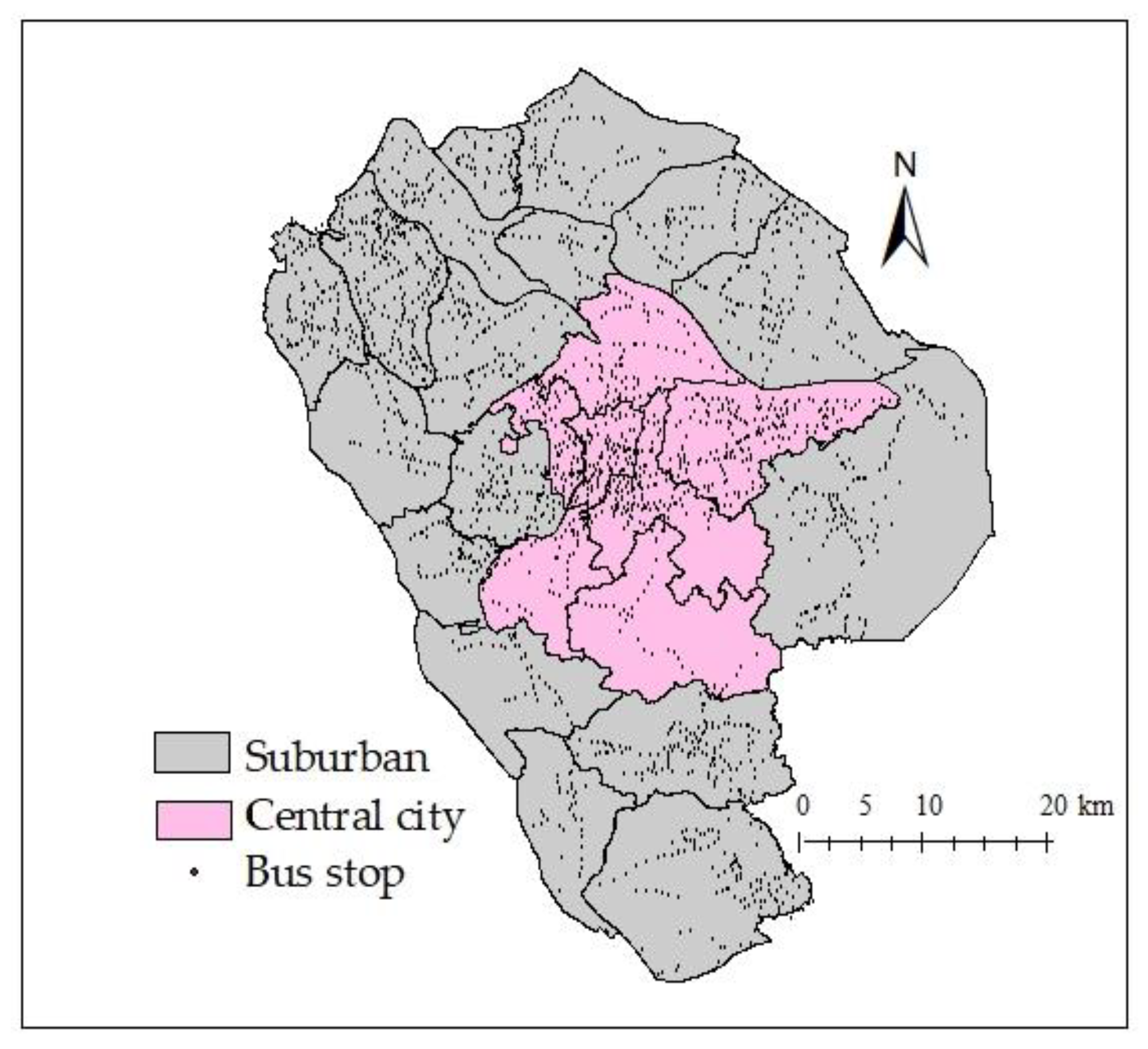
3.1. Data and Variables
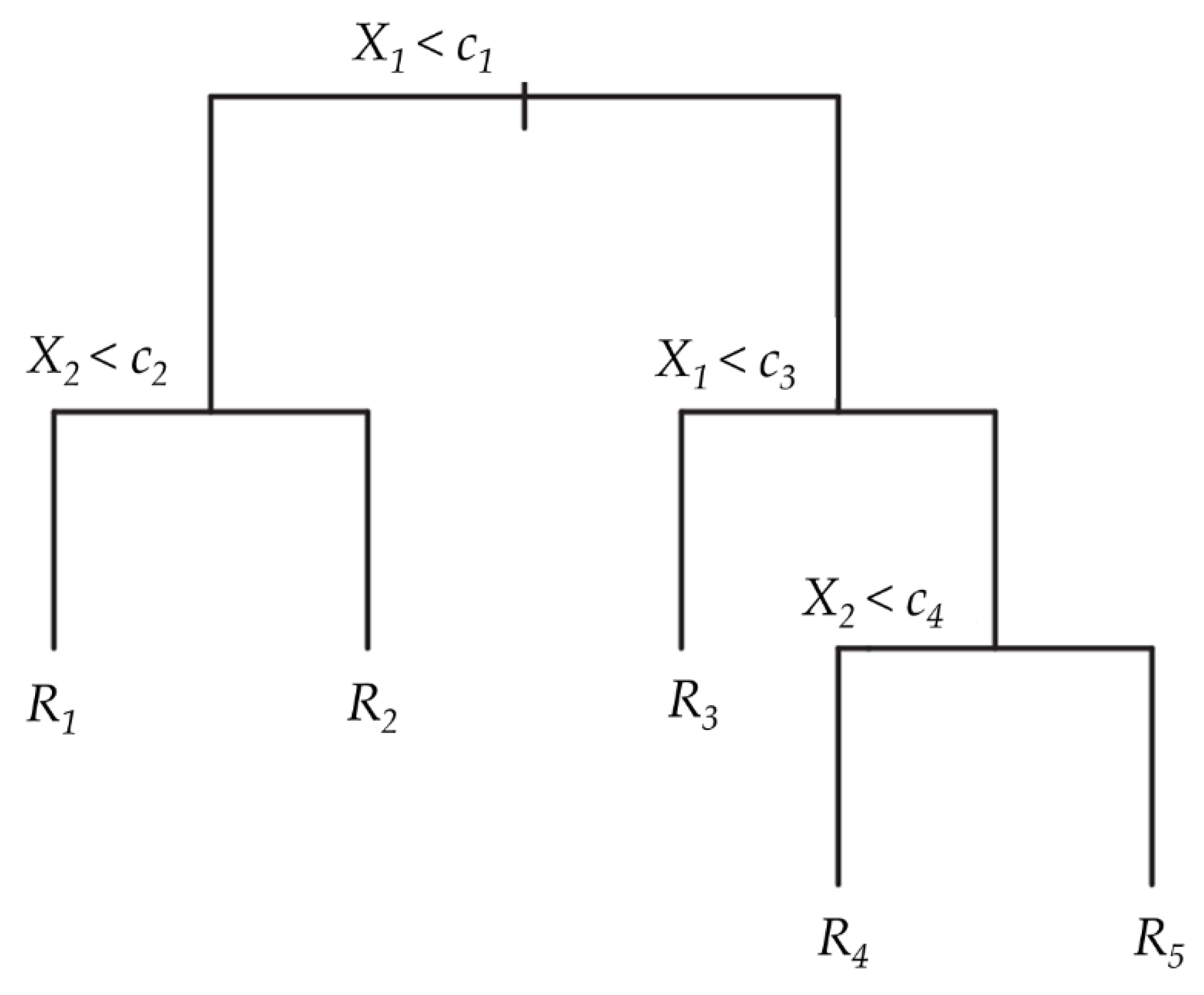
3.2. Modeling Approach
4. Results
4.1. Performance of the GBDT Model
4.2. Relative Importance of Independent Variables
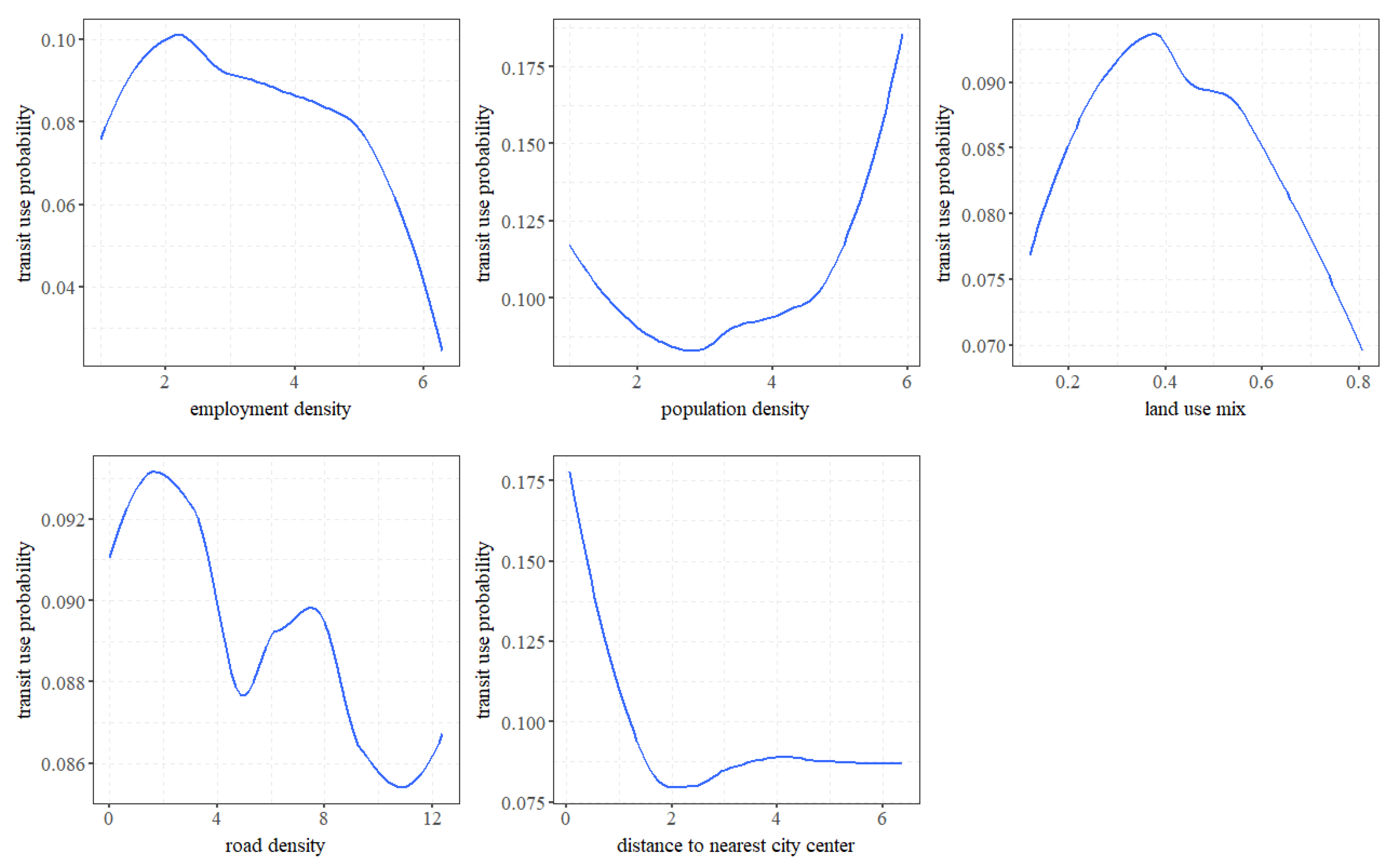
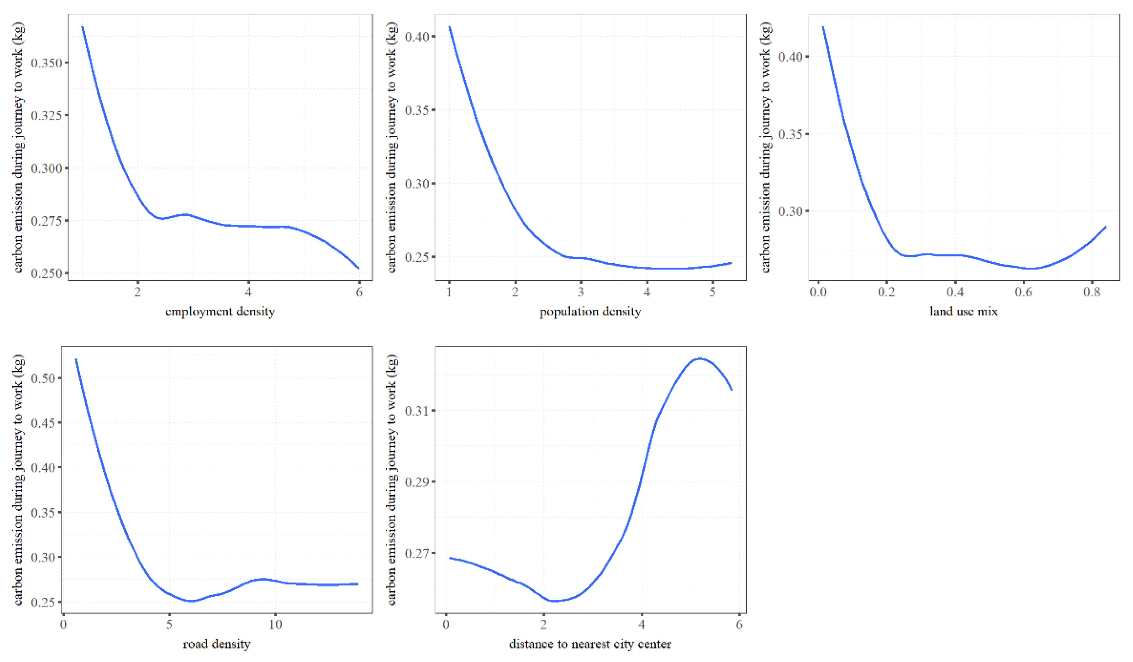
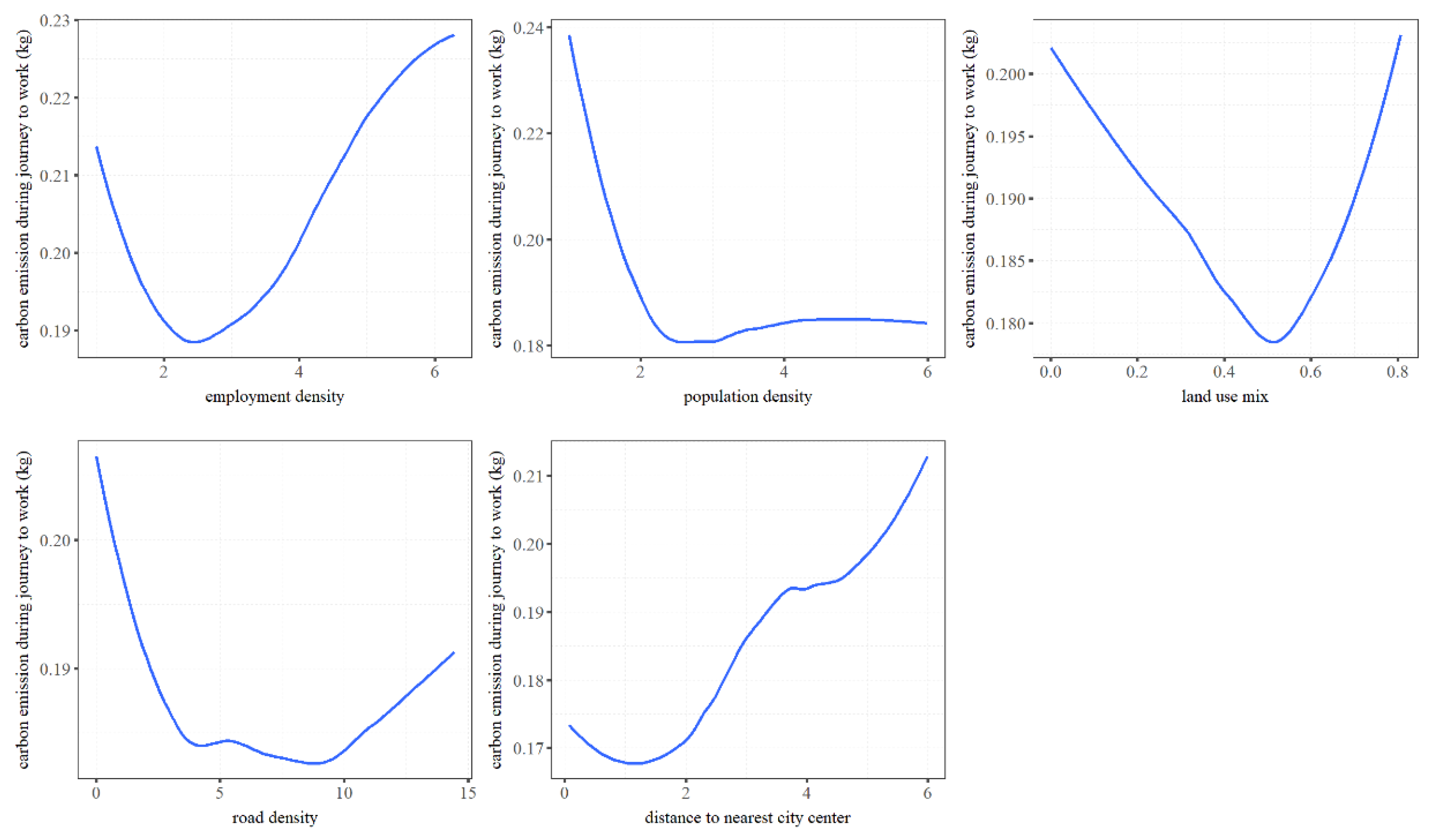
4.3. Nonlinear and Threshold Effects
4.4. The Stop Coverage Rate
5. Discussion and Conclusions
Author Contributions
Funding
Data Availability Statement
Conflicts of Interest
Appendix A

References
- Zuo, T.; Wei, H.; Chen, N. Promote transit via hardening first-and-last-mile accessibility: Learned from modeling commuters’ transit use. Transp. Res. Part D Transp. Environ. 2020, 86, 102446. [Google Scholar] [CrossRef]
- Gim, T.H.T. Analyzing the city-level effects of land use on travel time and CO2 emissions: A global mediation study of travel time. Int. J. Sustain. Transp. 2022, 16, 496–513. [Google Scholar] [CrossRef]
- Ewing, R.; Cervero, R. Travel and the built environment. J. Am. Plan. Assoc. 2010, 76, 265–294. [Google Scholar] [CrossRef]
- Park, K.; Ewing, R.; Sabouri, S.; Choi, D.; Hamidi, S.; Tian, G. Guidelines for a Polycentric Region to Reduce Vehicle Use and Increase Walking and Transit Use. J. Am. Plan. Assoc. 2020, 86, 236–249. [Google Scholar] [CrossRef]
- Yu, L.; Xie, B.; Chan, E.H.W. Exploring impacts of the built environment on transit travel: Distance, time and mode choice, for urban villages in Shenzhen, China. Transp. Res. Part E Logist. Transp. Rev. 2019, 132, 57–71. [Google Scholar] [CrossRef]
- Ma, J.; Liu, Z.; Chai, Y. The impact of urban form on CO2 emission from work and non-work trips: The case of Beijing, China. Habitat Int. 2015, 47, 1–10. [Google Scholar] [CrossRef]
- Sam Zimbabwe, E.G.; APTA. Defining Transit Areas of Influence; APTA Standards Development Program; American Public Transportation Association: Washington, DC, USA, 2009; p. 11. [Google Scholar]
- Le, J.; Ye, K. Measuring City-Level Transit Accessibility Based on the Weight of Residential Land Area: A Case of Nanning City, China. Land 2022, 11, 1468. [Google Scholar] [CrossRef]
- Yang, J.; Su, P.; Cao, J. On the importance of Shenzhen metro transit to land development and threshold effect. Transp. Policy 2020, 99, 1–11. [Google Scholar] [CrossRef]
- Galster, G.C. Nonlinear and Threshold Effects Related to Neighborhood: Implications for Planning and Policy. J. Plan. Lit. 2018, 33, 492–508. [Google Scholar] [CrossRef]
- Mwale, M.; Luke, R.; Pisa, N. Factors that affect travel behaviour in developing cities: A methodological review. Transp. Res. Interdiscip. Perspect. 2022, 16, 100683. [Google Scholar] [CrossRef]
- Tao, T.; Wang, J.; Cao, X. Exploring the non-linear associations between spatial attributes and walking distance to transit. J. Transp. Geogr. 2020, 82, 102560. [Google Scholar] [CrossRef]
- Guan, C.H.; Song, J.; Keith, M.; Akiyama, Y.; Shibasaki, R.; Sato, T. Delineating urban park catchment areas using mobile phone data: A case study of Tokyo. Comput. Environ. Urban Syst. 2020, 81, 101474. [Google Scholar] [CrossRef]
- Zhang, M. The role of land use in travel mode choice: Evidence from Boston and Hong Kong. J. Am. Plan. Assoc. 2004, 70, 344–360. [Google Scholar] [CrossRef]
- Shen, Q.; Chen, P.; Pan, H. Factors affecting car ownership and mode choice in rail transit-supported suburbs of a large Chinese city. Transp. Res. Part A Policy Pract. 2016, 94, 31–44. [Google Scholar] [CrossRef]
- Ao, Y.; Zhang, Y.; Wang, Y.; Chen, Y.; Yang, L. Influences of rural built environment on travel mode choice of rural residents: The case of rural Sichuan. J. Transp. Geogr. 2020, 85, 102708. [Google Scholar] [CrossRef]
- Zhao, P. The Impact of the Built Environment on Individual Workers’ Commuting Behavior in Beijing. Int. J. Sustain. Transp. 2013, 7, 389–415. [Google Scholar] [CrossRef]
- Ha, J.; Lee, S.; Ko, J. Unraveling the impact of travel time, cost, and transit burdens on commute mode choice for different income and age groups. Transp. Res. Part A Policy Pract. 2020, 141, 147–166. [Google Scholar] [CrossRef]
- Crotti, D.; Grechi, D.; Maggi, E. Proximity to public transportation and sustainable commuting to college. A case study of an Italian suburban campus. Case Stud. Transp. Policy 2022, 10, 218–226. [Google Scholar] [CrossRef]
- Kim, H.; Nam, J. The size of the station influence area in Seoul, Korea: Based on the survey of users of seven stations. Int. J. Urban Sci. 2013, 17, 331–349. [Google Scholar] [CrossRef]
- Alshalalfah, B.W.; Shalaby, A.S. Case Study: Relationship of Walk Access Distance to Transit with Service, Travel, and Personal Characteristics. J. Urban Plan. Dev. 2007, 133, 114–118. [Google Scholar] [CrossRef]
- Torres, M.A.; Oh, H.W.; Lee, J. The Built Environment and Children’s Active Commuting to School: A Case Study of San Pedro De Macoris, the Dominican Republic. Land 2022, 11, 1454. [Google Scholar] [CrossRef]
- Ding, C.; Cao, X.; Wang, Y. Synergistic effects of the built environment and commuting programs on commute mode choice. Transp. Res. Part A Policy Pract. 2018, 118, 104–118. [Google Scholar] [CrossRef]
- Viggiano, C.; Koutsopoulos, H.N.; Attanucci, J.; Wilson, N.H.M. Inferring public transport access distance from smart card registration and transaction data. Transp. Res. Rec. 2016, 2544, 55–62. [Google Scholar] [CrossRef]
- Guan, X.; Wang, D.; Jason Cao, X. The role of residential self-selection in land use-travel research: A review of recent findings. Transp. Rev. 2020, 40, 267–287. [Google Scholar] [CrossRef]
- Cao, X.; Xu, Z.; Fan, Y. Exploring the connections among residential location, self-selection, and driving: Propensity score matching with multiple treatments. Transp. Res. Part A Policy Pract. 2010, 44, 797–805. [Google Scholar] [CrossRef]
- Guerra, E.; Cervero, R.; Tischler, D. Half-mile circle: Does it best represent transit station catchments? Transp. Res. Rec. 2012, 2276, 101–109. [Google Scholar] [CrossRef] [Green Version]
- Ding, C.; Liu, T.; Cao, X.; Tian, L. Illustrating nonlinear effects of built environment attributes on housing renters ’ transit commuting. Transp. Res. Part D 2022, 112, 103503. [Google Scholar] [CrossRef]
- Cao, X.; Næss, P.; Wolday, F. Examining the effects of the built environment on auto ownership in two Norwegian urban regions. Transp. Res. Part D Transp. Environ. 2019, 67, 464–474. [Google Scholar]
- Ding, C.; Cao, X.; Næss, P. Applying gradient boosting decision trees to examine non-linear effects of the built environment on driving distance in Oslo. Transp. Res. Part A Policy Pract. 2018, 110, 107–117. [Google Scholar] [CrossRef]
- Lee, S.; Lee, B. Comparing the impacts of local land use and urban spatial structure on household VMT and GHG emissions. J. Transp. Geogr. 2020, 84, 102694. [Google Scholar] [CrossRef]
- Ao, Y.; Yang, D.; Chen, C.; Wang, Y. Effects of rural built environment on travel-related CO2 emissions considering travel attitudes. Transp. Res. Part D Transp. Environ. 2019, 73, 187–204. [Google Scholar] [CrossRef]
- Cao, X.; Yang, W. Examining the effects of the built environment and residential self-selection on commuting trips and the related CO2 emissions: An empirical study in Guangzhou, China. Transp. Res. Part D Transp. Environ. 2017, 52, 480–494. [Google Scholar] [CrossRef]
- Zhu, W.; Ding, C.; Cao, X. Built environment effects on fuel consumption of driving to work: Insights from on-board diagnostics data of personal vehicles. Transp. Res. Part D Transp. Environ. 2019, 67, 565–575. [Google Scholar] [CrossRef]
- Wang, X.; Liu, C.; Kostyniuk, L.; Shen, Q.; Bao, S. The influence of street environments on fuel efficiency: Insights from naturalistic driving. Int. J. Environ. Sci. Technol. 2014, 11, 2291–2306. [Google Scholar] [CrossRef] [Green Version]
- Boarnet, M.G.; Wang, X.; Houston, D. Can New Light Rail Reduce Personal Vehicle Carbon Emissions? a Before-After, Experimental-Control Evaluation in Los Angeles. J. Reg. Sci. 2017, 57, 523–539. [Google Scholar] [CrossRef]
- Gao, J.; Ma, S.; Li, L.; Zuo, J.; Du, H. Does travel closer to TOD have lower CO2 emissions? Evidence from ride-hailing in Chengdu, China. J. Environ. Manag. 2022, 308, 114636. [Google Scholar] [CrossRef] [PubMed]
- Shao, Q.; Zhang, W.; Jason, X.; Yang, J. Nonlinear and interaction effects of land use and motorcycles/E-bikes on car ownership. Transp. Res. Part D 2022, 102, 103115. [Google Scholar] [CrossRef]
- Wang, X.; Yin, C.; Zhang, J.; Shao, C.; Wang, S. Nonlinear effects of residential and workplace built environment on car dependence. J. Transp. Geogr. 2021, 96, 103207. [Google Scholar] [CrossRef]
- Yang, W.; Zhou, S. Using decision tree analysis to identify the determinants of residents’ CO2 emissions from different types of trips: A case study of Guangzhou, China. J. Clean. Prod. 2020, 277, 124071. [Google Scholar] [CrossRef]
- Wu, X.; Tao, T.; Cao, J.; Fan, Y.; Ramaswami, A. Examining threshold effects of built environment elements on travel-related carbon-dioxide emissions. Transp. Res. Part D Transp. Environ. 2019, 75, 1–12. [Google Scholar] [CrossRef]
- Kong, H.; Jin, S.T.; Sui, D.Z. Deciphering the relationship between bikesharing and public transit: Modal substitution, integration, and complementation. Transp. Res. Part D Transp. Environ. 2020, 85, 102392. [Google Scholar] [CrossRef]
- El-Geneidy, A.; Grimsrud, M.; Wasfi, R.; Tétreault, P.; Surprenant-Legault, J. New evidence on walking distances to transit stops: Identifying redundancies and gaps using variable service areas. Transportation 2014, 41, 193–210. [Google Scholar] [CrossRef]
- Yang, Y.; Wang, C.; Liu, W.; Zhou, P. Understanding the determinants of travel mode choice of residents and its carbon mitigation potential. Energy Policy 2018, 115, 486–493. [Google Scholar] [CrossRef]
- Zhang, W.; Lu, D.; Chen, Y.; Liu, C. Land use densification revisited: Nonlinear mediation relationships with car ownership and use. Transp. Res. Part D Transp. Environ. 2021, 98, 102985. [Google Scholar] [CrossRef]
- Zeng, J.; Qian, Y.; Mi, P.; Zhang, C.; Yin, F.; Zhu, L.; Xu, D. Freeway traffic flow cellular automata model based on mean velocity feedback. Phys. A Stat. Mech. Appl. 2021, 562, 125387. [Google Scholar] [CrossRef]
- Chakrabarti, S. How can public transit get people out of their cars? An analysis of transit mode choice for commute trips in Los Angeles. Transp. Policy 2017, 54, 80–89. [Google Scholar] [CrossRef]
- The 2006 IPCC Guidelines for National Greenhouse Gas Inventories. Available online: https://www.ipcc.ch/report/2019-refinement-to-the-2006-ipcc-guidelines-for-national-greenhouse-gas-inventories/ (accessed on 17 December 2022).
- Friedman, J.H. Greedy function approximation: A gradient boosting machine. Ann. Stat. 2001, 29, 1189–1232. [Google Scholar] [CrossRef]
- Tu, M.; Li, W.; Orfila, O.; Li, Y.; Gruyer, D. Exploring nonlinear effects of the built environment on ridesplitting: Evidence from Chengdu. Transp. Res. Part D Transp. Environ. 2021, 93, 102776. [Google Scholar] [CrossRef]
- Gan, L.; Ren, H.; Xiang, W.; Wu, K.; Cai, W. Nonlinear influence of public services on urban housing prices: A case study of China. Land 2021, 10, 1007. [Google Scholar] [CrossRef]
- Zhao, X.; Yan, X.; Yu, A.; van Hentenryck, P. Prediction and behavioral analysis of travel mode choice: A comparison of machine learning and logit models. Travel Behav. Soc. 2020, 20, 22–35. [Google Scholar] [CrossRef]
- Schonlau, M. Boosted regression (boosting): An introductory tutorial and a Stata plugin. Stata J. 2005, 5, 330–354. [Google Scholar] [CrossRef] [Green Version]
- Lambert, D. Zero-inflated poisson regression, with an application to defects in manufacturing. Technometrics 1992, 34, 1–14. [Google Scholar] [CrossRef]
- Cervero, R. Built environments and mode choice: Toward a normative framework. Transp. Res. Part D Transp. Environ. 2002, 7, 265–284. [Google Scholar] [CrossRef]
- Martin, E.W.; Shaheen, S.A. Evaluating public transit modal shift dynamics in response to bikesharing: A tale of two U.S. cities. J. Transp. Geogr. 2014, 41, 315–324. [Google Scholar] [CrossRef] [Green Version]
- Feng, R.; Feng, Q.; Jing, Z.; Zhang, M.; Yao, B. Association of the built environment with motor vehicle emissions in small cities. Transp. Res. Part D Transp. Environ. 2022, 107, 103313. [Google Scholar] [CrossRef]
- Hu, H.; Xu, J.; Shen, Q.; Shi, F.; Chen, Y. Travel mode choices in small cities of China: A case study of Changting. Transp. Res. Part D Transp. Environ. 2018, 59, 361–374. [Google Scholar] [CrossRef]
- Zhou, X.; Yeh, A.G.O.; Li, W.; Yue, Y. A commuting spectrum analysis of the jobs–housing balance and self-containment of employment with mobile phone location big data. Environ. Plan. B Urban Anal. City Sci. 2018, 45, 434–451. [Google Scholar] [CrossRef]
- Schwanen, T.; Dieleman, F.M.; Dijst, M. Travel behaviour in Dutch monocentric and policentric urban systems. J. Transp. Geogr. 2001, 9, 173–186. [Google Scholar] [CrossRef]
- Zhang, W.; Lu, D.; Zhao, Y.; Luo, X.; Yin, J. Incorporating polycentric development and neighborhood life-circle planning for reducing driving in Beijing: Nonlinear and threshold analysis. Cities 2021, 121, 103488. [Google Scholar] [CrossRef]
- Standard for Urban Comprehensive Transport System Planning. Available online: https://www.mohurd.gov.cn/gongkai/fdzdgknr/tzgg/201903/20190320_239844.html (accessed on 17 December 2022). (In Chinese)
- System of Assessment Indicators for Transit Metropolis. Available online: https://xxgk.mot.gov.cn/2020/jigou/ysfws/202006/t20200623_3314986.html. (accessed on 17 December 2022). (In Chinese)
- Qian, Y.; Zeng, J.; Wang, N.; Zhang, J.; Wang, B. A traffic flow model considering influence of car-following and its echo characteristics. Nonlinear Dyn. 2017, 89, 1099–1109. [Google Scholar] [CrossRef]
- Zeng, J.; Qian, Y.; Lv, Z.; Yin, F.; Zhu, L.; Zhang, Y.; Xu, D. Expressway traffic flow under the combined bottleneck of accident and on-ramp in framework of Kerner’s three-phase traffic theory. Phys. A Stat. Mech. Appl. 2021, 574, 125918. [Google Scholar] [CrossRef]
- Yang, J.; Cao, J.; Zhou, Y. Elaborating non-linear associations and synergies of subway access and land uses with urban vitality in Shenzhen. Transp. Res. Part A Policy Pract. 2021, 144, 74–88. [Google Scholar] [CrossRef]
- Cao, J.; Hao, Z.; Yang, J.; Yin, J.; Huang, X. Prioritizing neighborhood attributes to enhance neighborhood satisfaction: An impact asymmetry analysis. Cities 2020, 105, 102854. [Google Scholar] [CrossRef]
- Ma, Y.; Yang, Y.; Jiao, H. Exploring the impact of urban built environment on public emotions based on social media data: A case study of Wuhan. Land 2021, 10, 986. [Google Scholar] [CrossRef]
- Ding, C.; Cao, X.; Dong, M.; Zhang, Y.; Yang, J. Non-linear relationships between built environment characteristics and electric-bike ownership in Zhongshan, China. Transp. Res. Part D Transp. Environ. 2019, 75, 286–296. [Google Scholar] [CrossRef]
- Zeng, J.; Qian, Y.; Yin, F.; Zhu, L.; Xu, D. A multi-value cellular automata model for multi-lane traffic flow under lagrange coordinate. Comput. Math. Organ. Theory 2022, 28, 178–192. [Google Scholar] [CrossRef]
- Yao, Z.; Kim, C. The Changes of Urban Structure and Commuting: An Application to Metropolitan Statistical Areas in the United States. Int. Reg. Sci. Rev. 2019, 42, 3–30. [Google Scholar] [CrossRef]


| References | Study Area | Source | Walk, Bike | Electric Bike | Bus | Motorcycle | Car |
|---|---|---|---|---|---|---|---|
| Wu et al. (2019) [41] | Minneapolis, USA | U.S. Department of Transportation | 0 | - | 0.199 | - | 0.299 |
| Yang et al. (2018) [44] | Beijing, China | EC’s reports; Department of Energy and Climate Change in UK | 0 | 0.008 | 0.035 | - | 0.126 |
| Cao and Yang (2017) [33] | Guangzhou, China | Entwicklungsbank | 0 | - | 0.026 | - | 0.233 |
| Ao et al. (2019) [32] | Sichuan, China | Calculation from model proposed by EC; EC’ reports; Department of Energy and Climate Change in UK | 0 | 0.008 | 0.035 | 0.0472 | 0.126 |
| This study | Zhongshan, China | Same as Ao et al. (2019) [32] | 0 | 0.008 | 0.035 | 0.0472 | 0.126 |
| Name | Definition | Min. | Max. | Mean | St. Dev. | Source |
|---|---|---|---|---|---|---|
| Dependent variable | ||||||
| Transit use | A dummy variable indicating whether respondent chose to take bus | 0.00 | 1.00 | 0.02 | 0.14 | Travel survey |
| Carbon emissions | CO2 emitted during the commute to work, which equals Di ∗ Ri (kg) | 0.00 | 9.98 | 0.26 | 0.56 | Di from Baidu Map; Ri from Ao et al.’s work [32] |
| Key variable | ||||||
| Proximity to bus stop | Straight-line distance from house centroid to the nearest bus stop (m) | 1.30 | 3273.45 | 307.80 | 253.73 | Location from Baidu Map; Calculation using ArcGIS |
| Built environment | ||||||
| Employment density | Average employment density within 1-km buffer around the house (scale) | 1.00 | 6.29 | 2.55 | 1.05 | Baidu Map |
| Population density | Average employment density within 1-km buffer around the house (scale) | 1.00 | 6.00 | 2.46 | 1.00 | Baidu Map |
| Land use mix | Land use entropy | 0.00 | 0.84 | 0.49 | 0.14 | Land use data |
| Road density | Street length per km2 within 1-km buffer around the house (km/km2) | 0.00 | 14.45 | 6.63 | 2.88 | Land use data |
| Distance to the nearest city center | Straight-line distance from house centroid to nearest city center (km) | 0.06 | 9.47 | 2.58 | 1.56 | Land use data |
| Demographics | ||||||
| Gender | A dummy variable indicating whether respondent is female | 0.00 | 1.00 | 0.56 | 0.50 | Travel survey |
| Income | Level of respondent’s annual income: <50,000 noted as 0, 50–100,000 as 1, 100–200,000 as 2, >200,000 as 3 | 0.00 | 3.00 | 1.47 | 0.78 | Travel survey |
| Education | Level of respondent’s education: primary school noted as 0, junior high school as 1, senior high school as 2, vocational education as 3, bachelor and higher as 4 | 0.00 | 4.00 | 2.10 | 1.11 | Travel survey |
| Family size | Number of people in respondent’s family | 1.00 | 11.00 | 3.28 | 1.32 | Travel survey |
| Number of children | Number of respondent’s children | 0.00 | 5.00 | 0.39 | 0.63 | Travel survey |
| Area | Dependent Variables | GBDT | Traditional Regression Model |
|---|---|---|---|
| Central city | Transit use | 0.351 | 0.035 |
| Carbon emissions | 0.411 | 0.133 | |
| Suburban areas | Transit use | 0.613 | 0.035 |
| Carbon emissions | 0.192 | 0.067 |
| Predictor | Central City | Suburban Areas | ||||||
|---|---|---|---|---|---|---|---|---|
| Transit Use | Carbon Emissions | Transit Use | Carbon Emissions | |||||
| Relative Importance (%) | Ranking | Relative Importance (%) | Ranking | Relative Importance (%) | Ranking | Relative Importance (%) | Ranking | |
| Proximity to bus stop | 14.52 | 3 | 9.60 | 6 | 18.14 | 1 | 8.19 | 7 |
| Employment density | 15.82 | 1 | 11.48 | 4 | 13.35 | 3 | 9.54 | 5 |
| Population density | 12.15 | 6 | 13.01 | 3 | 11.59 | 6 | 9.15 | 6 |
| Land use mix | 13.70 | 5 | 10.24 | 5 | 12.35 | 4 | 11.49 | 3 |
| Road density | 14.67 | 2 | 5.84 | 8 | 11.67 | 5 | 11.38 | 4 |
| Distance to the nearest city center | 14.48 | 4 | 14.18 | 2 | 17.09 | 2 | 12.72 | 2 |
| Gender | 3.41 | 9 | 5.69 | 9 | 3.45 | 9 | 5.66 | 8 |
| Income | 2.11 | 10 | 7.80 | 7 | 1.37 | 11 | 5.38 | 9 |
| Education | 4.49 | 7 | 15.35 | 1 | 4.13 | 8 | 19.94 | 1 |
| Family size | 3.66 | 8 | 5.51 | 10 | 4.44 | 7 | 4.48 | 10 |
| Number of children | 0.98 | 11 | 1.29 | 11 | 2.44 | 10 | 2.07 | 11 |
| Suggested Level (m) | ||
|---|---|---|
| Central City | Suburban Areas | |
| Policy purpose | ||
| Promote transit use | 400 | 300 |
| Reduce carbon emission | 500 | 400 |
| Coverage Rate of Population (%) | Coverage Rate of Built Area (%) | |||
|---|---|---|---|---|
| Central City | Suburban Areas | Central City | Suburban Areas | |
| Policy purpose of criteria | ||||
| Current national criteria (500 m) | 93.8 | 83.8 | 83.3 | 73.5 |
| Promote transit use | 87.1 | 57.4 | 71.4 | 44.9 |
| Reduce carbon emissions | 93.8 | 74.0 | 83.3 | 61.5 |
Disclaimer/Publisher’s Note: The statements, opinions and data contained in all publications are solely those of the individual author(s) and contributor(s) and not of MDPI and/or the editor(s). MDPI and/or the editor(s) disclaim responsibility for any injury to people or property resulting from any ideas, methods, instructions or products referred to in the content. |
© 2022 by the authors. Licensee MDPI, Basel, Switzerland. This article is an open access article distributed under the terms and conditions of the Creative Commons Attribution (CC BY) license (https://creativecommons.org/licenses/by/4.0/).
Share and Cite
Hao, Z.; Peng, Y. Comparing Nonlinear and Threshold Effects of Bus Stop Proximity on Transit Use and Carbon Emissions in Developing Cities. Land 2023, 12, 28. https://doi.org/10.3390/land12010028
Hao Z, Peng Y. Comparing Nonlinear and Threshold Effects of Bus Stop Proximity on Transit Use and Carbon Emissions in Developing Cities. Land. 2023; 12(1):28. https://doi.org/10.3390/land12010028
Chicago/Turabian StyleHao, Zhesong, and Ying Peng. 2023. "Comparing Nonlinear and Threshold Effects of Bus Stop Proximity on Transit Use and Carbon Emissions in Developing Cities" Land 12, no. 1: 28. https://doi.org/10.3390/land12010028
APA StyleHao, Z., & Peng, Y. (2023). Comparing Nonlinear and Threshold Effects of Bus Stop Proximity on Transit Use and Carbon Emissions in Developing Cities. Land, 12(1), 28. https://doi.org/10.3390/land12010028