Physical Urban Area Identification Based on Geographical Data and Quantitative Attribution of Identification Threshold: A Case Study in Chongqing Municipality, Southwestern China

Abstract

Although some methods have identified the physical urban area to a certain extent, the driving factors for the identification threshold have not been studied deeply. In this paper, vector building data and road intersection data are used for comparative validation based on the urban expansion curve method to identify the physical urban area using the meso-city scale. The geographical detector technique is used to detect how and to what extent the urban spatial structure factors, geographical environment factors and social economic factors affect the optimal distance threshold of 22 administrative districts in the Chongqing municipality. The results based on the vector buildings are more precise and show the characteristics of the physical urban area of core-periphery distribution and the distribution along the water corridor. From the results of quantitative attribution, it was found that the road network density, building density, urbanization rate and urban population density, and their interaction with regional GDP, play a critical role in the optimal distance threshold, with the index value of influence degree ≥0.79. Under the influence of different factors, the optimal distance thresholds of 22 administrative districts show adaptive characteristics. Looking forward to the future, this study provides ideas for further research on the morphological characteristics and distribution laws of multi-spatial scale cities.

1. Introduction

Urban and rural statistical work in China mainly takes the administrative scope as the basic statistical unit, but there is a phenomenon where the urban statistical scope is separated from the natural geographical scope, which can objectively reflect the distribution of the urban rank scale [1,2]. In order to accurately distinguish cities and villages, it is necessary to identify the physical urban area from bottom to top. In China, physical urban areas are similar to built-up areas, including not only concentrated and contiguous core urban areas but also some scattered urban areas closely related to core urban areas. It has comparability with the international concept of urbanized areas [3,4]. The urban built-up area has a dynamic dataset including time and space characteristics, which is the official standard statistical data of the “China Urban Construction Statistical Yearbook” [5,6]. It is not a city in the administrative sense but a city in the actual landscape [7]. In the identification of the physical urban area, the built-up area is often used as the standard for error of test results. Only by accurately identifying the physical urban area can the urban spatial information be correctly extracted, and the conclusions drawn from it truly reflect the urban characteristics, so as to better carry out the qualitative and quantitative analysis of the city [8].

For the physical urban area, earlier research used statistical data such as population, economy, gross domestic product (GDP) and other data to identify it [9,10]. However, However, due to low timeliness, long period and poor objectivity of statistical data [11], urban areas could not be accurately identified. The present research used remote sensing product such as remote sensing images [12,13,14] and nighttime light data [15,16,17] to identify the physical urban area. Although the identification results of image data are of high precision, and the nighttime light data can reflect the spatial variations of urban development on a large scale, they all show the urban form as formed by artificial identification. Moreover, the remote sensing interpretation method relies on certain subjective judgment experiences. There is also no comparability between thresholds in different regions with nighttime light data [18]. In contrast, the study data used by Jiang et al. [19,20,21] and Tannier et al. [22,23] are street nodes (intersection points and endpoints) data and vector map building data. The two kinds of geographical data are the basic elements of urban spatial structure; its concentration closely relates to human activities and directly reflects the pattern and size of the city. Based on fractal geometry, the Minkowski dilation method used by Tannier can identify the urban boundary at different scales without a predefined threshold. Fractal geometry and its related concepts are an effective means to describe urban scale and form [24] and can provide powerful tools for studying the spatial organization of urban patterns [25].

The above geographic data combined with the urban expansion curve method can objectively identify natural cities from the bottom up, and the identification threshold of different cities can be compared [22]. Different cities have different optimal distance thresholds due to different driving factors. So, it is very attractive to explore the law of the optimal distance threshold for different cities. However, some existing studies [5,18] only used the optimal distance threshold to identify a physical urban area with high precision, and no further research was conducted. Tannier also only analyzed how different thresholds in different cities were influenced by factors such as distances separating buildings, road network density, population size and economic policies, and did not quantitatively analyze the relationship between these factors and the optimal distance threshold. Through quantitative analysis of the driving factors of different optimal distance thresholds, the intrinsic driving mechanism and change rule can be found, and the spatial organization characteristics and distribution patterns of different regions also can be revealed. This hopes to provide a data basis for rational planning of urban construction land and a special perspective on the study of natural laws of spatial morphology development and structural layout in different regions.

Therefore, based on the vector building data, this paper firstly uses the urban expansion curve method to identify the optimal distance threshold, and extract the physical urban area using the meso-city scale. Secondly, the correlation analysis [26], multiple regression analysis [27] and principal component analysis [28] are no longer used to analyze the single effect of independent variables on the dependent variable. Using the geographical detector method [29], it detects the comprehensive influence from urban spatial structure factors, geographical environmental factors and socio-economic factors on the micro-district scale on the optimal distance thresholds. At last, for comparative validation to obtain the most accurate optimal distance threshold, the built-up area and satellite images were used as reference standards to compare the identification results based on the vector building data with that based on the road intersection data. As the only municipality directly under the central government in southwestern China, this paper selected 22 districts of different levels in the Chongqing municipality to explore the morphological characteristics and distribution laws from the medium-micro scale. Its spatial organization structure is similar to that of urban agglomerations containing different levels of cities. This provides ideas for the quantitative urban study on macro-medium spatial scales such as urban agglomerations with different levels of cities or broader spatial scales.

2. Materials and Methods

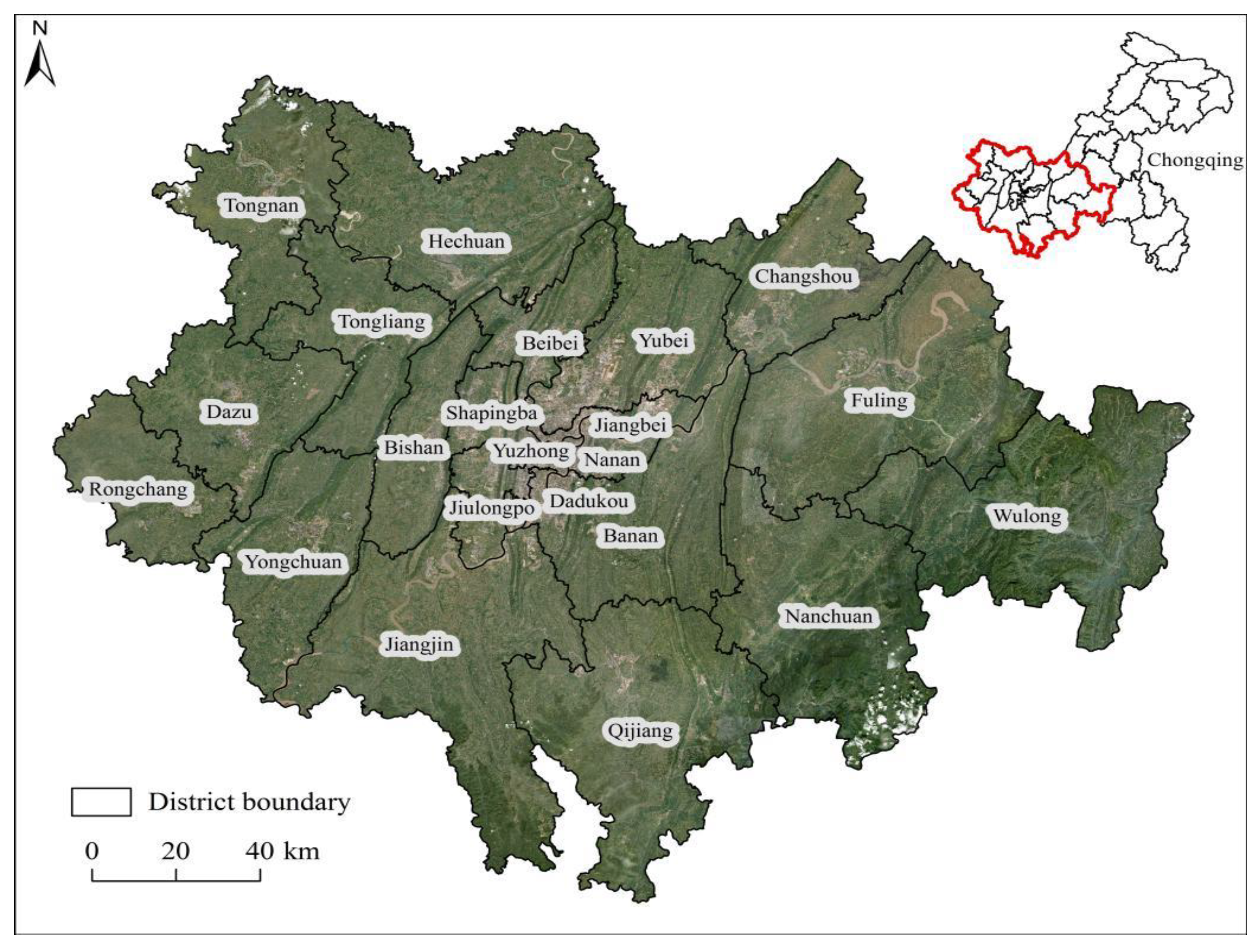
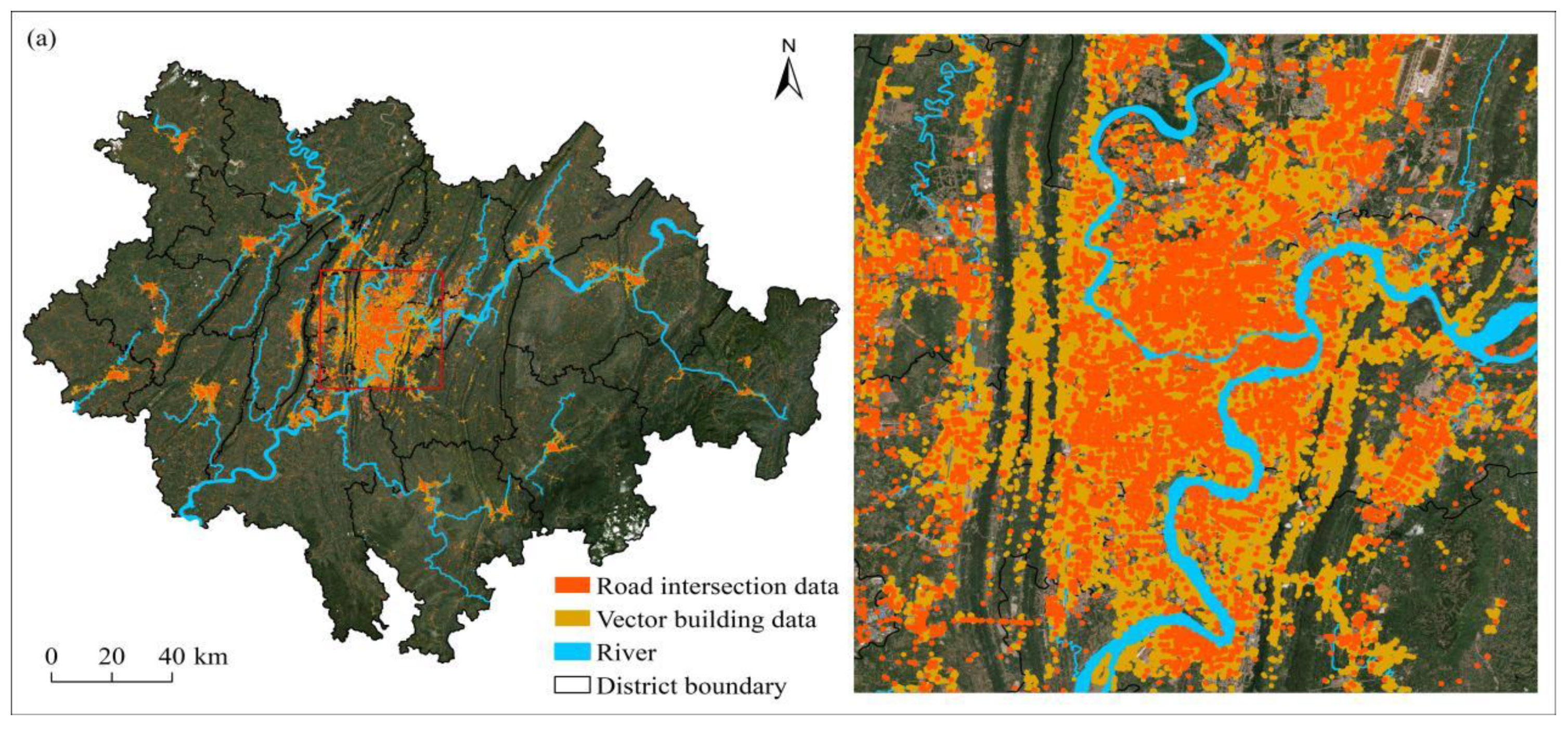
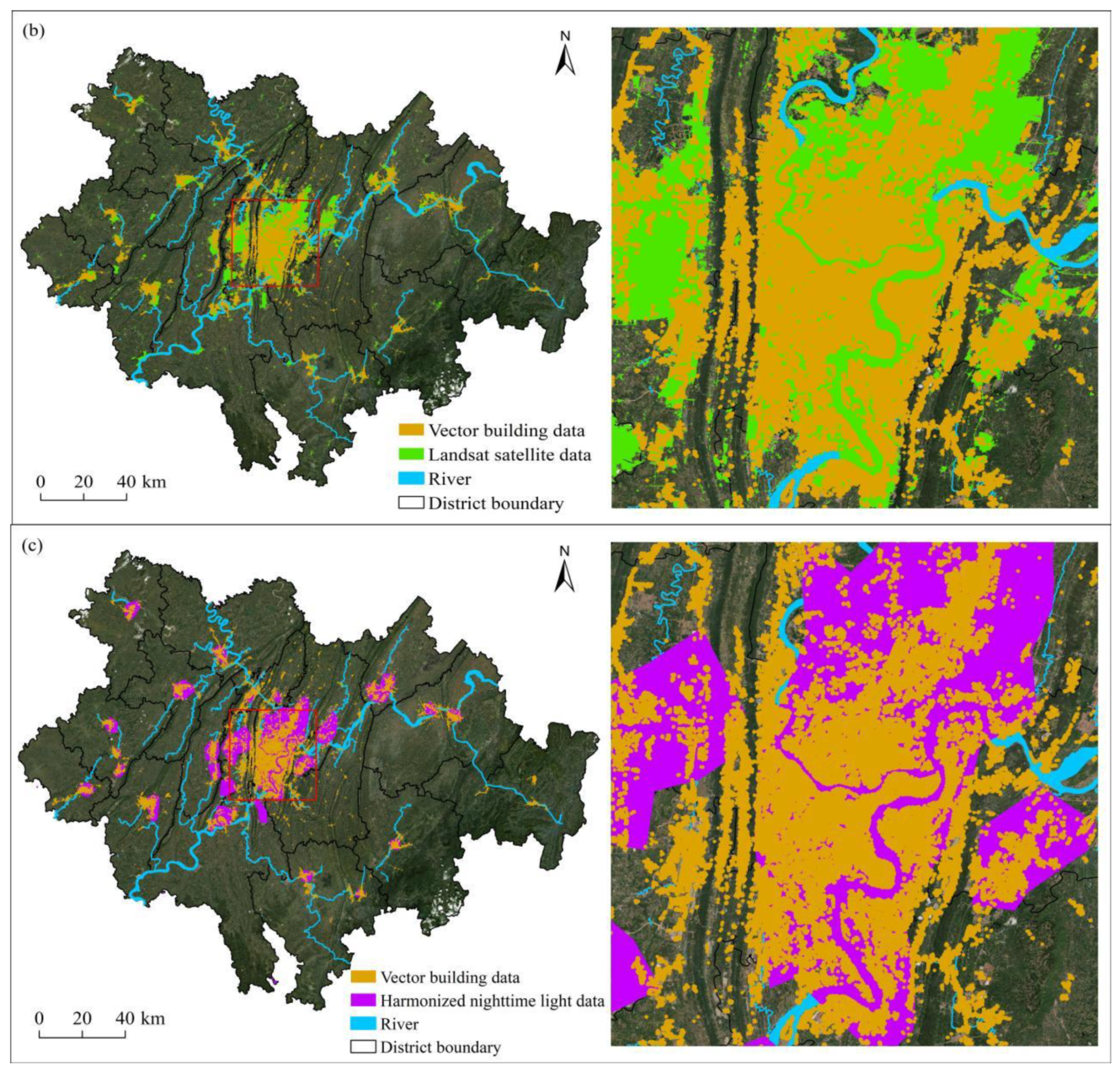
2.1. Study Area and Data Sources

As a mountain city, the Chongqing municipality covers an area of 82,400 square kilometers and has a permanent population of 32,1243 million, with an economic aggregate of 2.36 trillion yuan at the end of 2019. In this paper, 9 centrally distributed central urban areas, which are the main urban concentrated areas with good economic development, and 13 dispersed peripheral districts affected by central urban areas were selected as the research objects to identify the physical urban area and quantitatively attribute the optimal distance threshold (Figure 1).

OpenStreetMap (OSM) (https://www.openstreetmap.org/, accessed on 1 November 2020) and electronic maps were shared, alongside innovative map data with massive vector data [30,31]. This paper trawled and downloaded the building and road network of 22 administrative districts in the Chongqing municipality in 2020 from electronic maps API and OpenStreetMap (OSM). The complete building and road network data were obtained by fusion processing, and 79,813 road intersections and 39,8151 vector building patches were obtained by deduplication, screening and geometric repair in ArcGIS. Part of the vector building data and road intersection data extracted from the road network are shown in (Figure 2).

The road network density, building density, topographic relief, ratio of river size to district area (hereinafter referred to as the river area ratio), urban population density, urbanization rate and regional GDP were selected from the urban spatial structure, geographical environment and socio-economic factors for geographical detection analysis with the optimal distance thresholds. Road network density and building density were obtained by dividing road network length, building area and total area of each district; topographic relief was calculated from ALOS-12.5 m DEM in the Chongqing municipality; the river area ratio was obtained by dividing the river area and the total area of each district; the data of urban population density, urbanization rate and regional GDP come from the “2020 Chongqing Statistical Yearbook”. The built-up area of 22 districts comes from the 2020 statistical yearbooks, statistical bulletins, the vector map of satellite images in 10 m resolution and the planning bureau of each district to verify the accuracy of the physical urban area (

Table 1. Driving factors in 22 administrative districts.

District	Built-Up Area/km2	Road Network Density/(km/km2)	Building Density/%	Topographic Relief/m	River Area Ratio/%	Urban Population Density/(Million People/km2)	Urbanization Rate/%	Regional GDP/(Billion Yuan)
Ba’nan	105.38	1.64	0.23	148	2.31	0.05	82.71	875
Beibei	65.66	1.72	0.48	104	2.32	0.09	84.50	606
Bishan	33.73	1.96	0.22	62	0.57	0.05	60.20	681
Dadukou	35.99	2.56	1.54	69	11.16	0.34	97.71	254
Dazu	30.09	1.75	0.15	95	0.34	0.03	60.05	646
Fuling	72.01	1.64	0.07	200	3.28	0.03	69.77	1179
Hechuan	49.02	1.44	0.09	158	3.67	0.04	70.59	913
Jiangbei	101.12	2.58	1.43	118	10.07	0.39	96.50	1240
Jiangjin	87.6	1.27	0.05	199	3.17	0.03	69.76	1037
Jiulongpo	132.09	2.56	1.54	58	2.65	0.27	94.14	1463
Nan’an	90.88	2.71	1.36	111	8.31	0.34	96.03	771
Nanchuan	26.55	1.19	0.04	273	0.22	0.01	62.35	334
Qijiang	26.89	1.53	0.07	198	0.53	0.03	64.08	683
Rongchang	21.68	1.94	0.15	63	0.47	0.04	58.36	653
Shapingba	121.08	2.67	1.46	64	1.71	0.28	95.97	977
Tongliang	20.46	1.95	0.12	79	0.78	0.03	58.36	617
Tongnan	30.46	1.60	0.06	72	0.80	0.03	55.56	451
Wulong	6.58	1.57	0.02	288	0.69	0.01	45.55	210
Yongchuan	80.4	1.92	0.14	114	1.00	0.05	71.27	953
Yubei	202.44	1.91	0.53	119	1.62	0.1	84.22	1848
Yuzhong	17.62	5.76	4.80	74	21.13	2.89	100.00	1301
Changshou	54.5	1.82	0.17	109	1.96	0.04	67.82	701

). According to the characteristics and attributes of driving factors, the method of equal step classification and natural breaks were used to partition them for spatial heterogeneity detection in GEO detectors. The specific partition (

Table 2. Driving factor partition description in geographic detector.

Driving Factors	Number of Partitions	Partition Description
Road network density/(km/km2)	1~4	1. 1.19~1.69; 2. 1.69~2.20; 3. 2.20~2.71; 4. 2.71~5.76
Building density/%	1~4	1. 0.02~0.52; 2. 0.52~1.03; 3. 1.03~1.54; 4.1.54~4.80
Topographic relief/m	1~6	1. 58~96; 2. 96~134; 3. 134~173; 4. 173~211; 5. 211~249; 6. 249~288
River area ratio/%	1~6	1. 0.22~3.70; 2. 3.70~7.19; 3. 7.19~10.67; 4. 10.67~14.16; 5. 14.16~17.64; 6. 17.64~21.13
Urban population density/(million people/km2)	1~4	1. 0.01~0.13; 2. 0.13~0.26; 3. 0.26~0.39; 4. 0.39~2.89
Urbanization rate/%	1~5	1. 45.55~56.44; 2. 56.44~67.33; 3. 67.33~78.22; 4. 78.22~89.11; 5. 89.11~100
Regional GDP/(billion yuan)	1~5	1. 210~537; 2. 537~865; 3. 865~1192; 4. 1192~1520; 5. 1520~1848

) and spatial distribution (Figure 3) of 7 driving factors were obtained.

2.2. Research Methods

2.2.1. Urban Expansion Curve Method

The urban expansion curve method, based on fractal theory to identify the physical urban area, mainly included two steps. The first step was to obtain the urban expansion curve with X as the buffer radius and Y as the cluster numbers. Tannier analogized buildings and streets in real urban structures to black squares separated by white empty lanes in a fractal structure of Fourier Dusts. According to Minkowski dilation [32,33], there is a power function law between the size and the number of white empty lanes, and between the size of the black square and its number. That is, with the widening of the buffer zone, the buildings or streets surrounded by the buffer zones become merged and clusters form, and the number of clusters gradually decreases until it is 1 and stops expansion in the real city. There is a power-law relationship between the buffer radius and cluster numbers, which are X and Y of the urban expansion curve:

$$N=a*r^D$$

(1)

where N is the number of clusters, a is a constant, r is the buffer radius, and D is the fractal dimension. The logarithm was taken on both sides of the equation to obtain the double logarithmic curve with D as the slope, and there is a linear relationship between log(r) and log(N):

$$log\left(N\right)=D*log\left(r\right)+log\left(a\right)$$

(2)

The second step was to obtain the optimal distance threshold, which corresponds to the principal curvature point. The double logarithmic curve of the buffer radius cluster number was fitted using a polynomial. The curvature of each point on the expansion curve was calculated according to the curvature calculation formula [22,34]. The curvature extreme point with the maximum absolute value was the principal curvature point, and the corresponding buffer radius was the optimal distance threshold. It divided the city into two spatial subsets. Within the optimal distance threshold, it was the city of self-similar. Outside the optimal distance threshold, it was always rural, and there was no self-similarity or self-similarity with insignificant changes [23]. Thus, the physical urban area was identified.

$$K=\frac{y^{″}}{{\left(1+{y^{\prime }}^2\right)}^{3/2}}$$

(3)

where K is the curvature of each point on the urban expansion curve; y′ is the first derivative of the polynomial fitting curve; y″ is the second derivative of the polynomial fitting curve.

2.2.2. Geographical Detector Method

The geographic detector method analyzes the influence of different explanatory variables on dependent variables. Its core idea is that if an independent variable has an important influence on a dependent variable, the spatial distribution of the independent variable and the dependent variable should be similar or consistent [29,35]. It mainly includes a factor detector, an ecological detector and an interactive detector. A factor detector detects the explanatory power of different independent variables X to dependent variable Y. Using a q value to measure q value changes between 0–1, the greater the value represents the greater the influence of X on Y. Ecological detection is used to detect whether the influence of different independent variables X on the dependent variable Y is significantly different. The interactive detector is to detect whether the influence of two or more factors on dependent variable Y is significantly greater or smaller than that of a single factor, and whether the influence of these factors on dependent variable Y is independent. There are five types of interactions between two different driving factors (

Table 3. Types of intersections in interactive detection.

Description	Intersection
q(A∩B) > max(q(A), q(B))	Enhance, bivariate
q(A∩B) < min(q(A), q(B))	Weaken, nonlinear
q(A∩B) = q(A) + q(B)	Independent
q(A∩B) > q(A) + q(B)	Enhance, nonlinear
min(q(A), q(B)) < q(A∩B) < max(q(A), q(B))	Weaken, bivariate

).

$$q=1-\frac{1}{N{\sigma }^2}{\displaystyle \sum }_{i=1}^L{N}_i{\sigma }_i^2$$

(4)

where q is the spatial heterogeneity of an index, N is the total number of samples in the study area, σ² is the variance of the index, i is the partition, and L is the number of partitions.

3. Results

3.1. Identification of Optimal Distance Threshold

For the buffer analysis based on vector building data, the initial buffer distance was set to 20 m and increased by twice the speed, and the number of clusters was counted after each dilation step. By fitting the double logarithmic curve of the buffer radius and the number of building clusters, the curvature was calculated by the curvature calculation formula, and the principal curvature point and corresponding distance threshold were obtained (

Table 4. Curvature extremum corresponding to distance threshold.

Region	Principal Curvature Point	Optimal Distance Threshold/m
Chongqing Municipality	0.36	146
Ba’nan	−0.12	46
Beibei	0.03	89
Bishan	−0.26	57
Dadukou	−0.14	102
Dazu	−0.28	45
Fuling	−0.96	36
Hechuan	−0.06	52
Jiangbei	0.08	176
Jiangjin	−0.25	50
Jiulongpo	0.10	169
Nan’an	0.06	132
Nanchuan	−0.58	39
Qijiang	−0.22	52
Rongchang	−0.31	38
Shapingba	0.04	149
Tongliang	−0.20	42
Tongnan	0.01	52
Wulong	−0.81	32
Yongchuan	0.02	49
Yubei	0.11	104
Yuzhong	−0.06	111
Changshou	−0.14	64

). It was shown that the principal curvature points were between −0.96 and 0.11, and the corresponding optimal distance thresholds were within the range of 32–176 m among the 22 districts. The optimal distance thresholds of the Dadukou district, Jiangbei district, Jiulongpo district, Nan’an district, Shapingba district, Yubei district and Yuzhong district were all larger than 100 m, while the others were less than 100 m. However, due to the common influence of the 22 districts, the principal curvature point in the Chongqing municipality was 0.36, and the corresponding optimal distance threshold of 146 m was between 32 m and 176 m.

3.2. Identification of Physical Urban Area

The principal curvature point 0.36 with the corresponding buffer radius 146 m was the optimal distance threshold on the meso-city scale. After which the physical urban area was formed by buffering at 146 m. Superimposed satellite images were used to obtain the map of the physical urban area in the Chongqing municipality (Figure 4). As shown in the figure, under the optimal distance threshold, most vector buildings have fused to form a concentrated and contiguous physical urban area. The distribution pattern of the whole city presents the characteristics of core-periphery distribution and distribution along the water corridor. The characteristics of the core-periphery distribution were mainly reflected in the 9 central districts of the Chongqing municipality, which are the core area of the city. Among the 9 central districts, the Yuzhong district is the core area and radiates to the other 8 districts, with the 13 periphery districts distributed around the 9 districts, forming the core-periphery urban distribution characteristics. The characteristics of the distribution along the water corridors were mainly shown in the 9 central districts that are concentrated at the intersection of the Yangtze River and the Jialing River. Most of the urban clusters in the 13 peripheral districts were also concentrated along the main streams and tributaries of the two rivers, forming a strip shape along the river, which is generally characterized by the distribution along the water corridors.

3.3. Analysis of Driving Factors of Optimal Distance Threshold

3.3.1. Factor Detection Analysis

Factor detection results were analyzed (Figure 5). The influence degree of all driving factors on the optimal distance threshold was as follows: building density (0.85) > urbanization rate (0.83) > road network density (0.81) > urban population density (0.79) > regional GDP (0.50) > river area ratio (0.38) > topographic relief (0.29). Among them, building density, urbanization rate, road network density and urban population density all had a great influence on the optimal distance threshold, and the index values of their influence degree were relatively close and had a fault with the index values of the other three factors. The higher the building density, urbanization rate, road network density and urban population density, the greater the optimal distance threshold. The impact of regional GDP as an economic factor on the optimal distance threshold was much smaller than that of the other two economic factors. In addition, the influence of the river area ratio and topographic relief on the optimal distance threshold was the smallest, but they also influence the optimal distance threshold to some extent.

3.3.2. Ecological Detection Analysis

Ecological detector results were analyzed (

Table 5. Ecological detection results.

Driving Factors	Road Network Density	Building Density	Topographic Relief	River Area Ratio	Urban Population Density	Urbanization Rate
Building density	N
Topographic relief	Y	Y
River area ratio	Y	Y	N
Urban population density	N	N	Y	Y
Urbanization rate	N	N	Y	Y	N
Regional GDP	Y	Y	N	N	Y	Y

). There were significant differences in the impact of urban spatial structure factors and geographical environment factors on the optimal distance threshold. Except for regional GDP, urban spatial structure factors and geographical environment factors showed no significant differences to the other two economic factors. The functional attributes of the two factors in urban spatial structure were similar, and there were no significant differences in their impact on the optimal distance threshold, or on the geographical environment factors. However, there were significant differences between regional GDP and the other two socio-economic factors.

3.3.3. Interactive Detection Analysis

Interactive detector results were analyzed (

Table 6. Interactive detection results.

Driving Factors	Road Network Density	Building Density	Topographic Relief	River Area Ratio	Urban Population Density	Urbanization Rate	Regional GDP
Road network density	0.81
Building density	0.87	0.85
Topographic relief	0.88	0.90	0.29
River area ratio	0.88	0.91	0.52	0.38
Urban population density	0.82	0.86	0.88	0.85	0.79
Urbanization rate	0.90	0.88	0.90	0.91	0.86	0.83
Regional GDP	0.95	0.95	0.87	0.76	0.95	0.93	0.50

). The interaction of any two driving factors was greater than the influence of any single factor, and there was no independent interaction between each factor. While the interaction between the topographic relief and regional GDP was nonlinear, the interaction between any two other factors was bilinear. Among them, the most obvious combination of bilinear enhancement was the river area ratio with a q of 0.38 and regional GDP with a q of 0.5, and the difference between the q value of 0.76 after their interaction and the maximum value of 0.5 of the single effect was the largest. For the factors with a large q value, the interaction was also large. The interaction of urban spatial structure factors and urban population density with regional GDP has the greatest impact on the change in the optimal distance threshold, with a q value of 0.95. Followed by the interaction between the urbanization rate and regional GDP, the q value is 0.93. In addition, the pairwise interaction of urban spatial structure factors with geographical environment factors, urban population density and urbanization rate had a significant influence on the optimal distance threshold, with the q value varying between 0.82 and 0.91. Compared with the interaction of other factors, the q value obtained by the interaction between socio-economic factors and geographical environment factors was significantly enhanced but fluctuated greatly.

3.3.4. Adaptiveness of Optimal Distance Threshold

By analyzing the correlation between the optimal distance threshold and 7 driving factors, it was found that when the q value of the factor detector is ≥0.79, the corresponding optimal distance threshold is >100 m for administrative districts with road network density, building density, urban population density and urbanization rates >2, >1, >0.2 and >90%, respectively. When road network density, building density, urban population density and urbanization rate are <2, <1, <0.2 and <90%, respectively, the optimal distance threshold is <100 m for other districts except the Yubei district, since the optimal distance threshold of a city cannot be within a few meters or more than several kilometers away. Combined with the law of the optimal distance threshold of the 22 administrative districts, it corresponds to the two stages of the urban expansion process, namely the buffer radiuses of 20–100 m and 100–1000 m. Among the 22 administrative districts, 7 districts, the Dadukou district, the Jiangbei district, the Jiulongpo district, the Nan’an district, the Shapingba district, the Yubei district and the Yuzhong district, had an optimal distance threshold at the stage of 100–1000 m, the stage at which the physical urban area is also formed. This was due to the high road network density, building density, urban population density and urbanization rate. Fifteen districts, the Ba’nan district, the Beibei district, the Bishan district, the Dazu district, the Fuling district, the Hechuan district, the Jiangjin district, the Nanchuan district, the Qijiang district, the Rongchang district, the Tongliang area, the Tongnan district, the Wulong district, the Yongchuan district, and the Changshou district, all have a relatively low road network density, building density, urban population density and urbanization rate, with the optimal distance threshold at the stage of 20–100 m, at which stage the physical urban area is also formed. This change rule shows the adaptability characteristics of the optimal distance threshold and reflects the distribution law of the city.

4. Discussion

4.1. Accuracy Verification of Physical Urban Area

For accuracy verification, area error and image overlay were used as the two standards, and a contrast test was developed between the identification results of vector buildings and those based on road intersections. The results of the optimal distance threshold and area error were obtained (

Table 7. Comparison of four data.

Data	Optimal Distance Threshold/m	Physical Urban Area/km2	Built-Up Area/km2	Area Error Rate/%
Vector building	146	1598.43	1412.23	13.18%
Road intersection	156	1112.79		−21.2%
Landsat satellite	none	2081.85		47.42%
Harmonized nighttime light	none	1948.17		37.95%

). It was shown that the optimal distance threshold based on road intersection data was larger than that based on vector building data. Because the width of a street is generally smaller than that of a building [36,37], the interval between road intersections was larger than that between vector buildings. There were differences in the shape and size of road intersections and vector buildings, and within a certain range, the density of road intersections was smaller than that of vector buildings. Therefore, in the expansion process, vector buildings only needed a smaller buffer radius to fuse the separated buildings, thus forming a real physical urban area with a smaller optimal distance threshold. By comparing the error of the physical urban area, combined with the comparison map of the physical urban area based on two kinds of data (Figure 6), it is obvious that the error 13.18% for the physical urban area extracted based on vector building data was smaller than the 21.2% for the physical urban area extracted based on the road intersection. The main reason for the larger built-up area is that some green park spaces were included in the process of the fusion of vector buildings to form the physical urban area. There are many single clusters that could not merge with neighboring clusters to form a concentrated urban cluster, resulting in the identification of an incomplete physical urban area based on road intersections. The figure shows how the vector buildings and road intersections have formed roughly similar urban patterns. The physical urban area based on the vector building was more concentrated and contiguous and roughly coincided with the urban built-up area on the image, whereas there were many holes in the identification results based on road intersections.

Comparison with other identification results using different data and methods, impervious surface dataset [38] extracted from Landsat satellites with a spatial resolution of 30 m (http://irsip.whu.edu.cn/resources/dataweb.php, accessed on 1 December 2020) and an urban extent dataset [39] extracted from Harmonized nighttime lights (https://doi.org/10.6084/m9.figshare.16602224.v1, accessed on 1 December 2020) were downloaded. After processing in ArcGIS, the physical urban area of the Chongqing municipality identified by these two different data were obtained (Table 7). As is shown, the physical urban area extracted from the Landsat satellites and Harmonized nighttime lights data were all larger than the built-up area, with the area errors of 47.42% and 37.95%, respectively, which was also larger than that based on vector building data. With satellite images as the base map, it was found that the physical urban areas identified by the two different data contained many areas that do not represent cities. The identification results only show the overall outline of the city, while the identification results based on vector buildings can better reflect the spatial details inside the city (Figure 6). In general, it can be seen that the vector building data selected in this paper better reflects the layout and structure of the city, and the extracted physical urban area is more accurate. Furthermore, the urban expansion curve method based on fractal theory is a self-organizing process without artificial presupposition [40,41], which does not require complex operation steps, making the identification of the optimal distance threshold more objective and reliable. In addition, the area error of the Fuling district, the Jiangjin district and the Yongchuan district were between 30% and 40%, the area error of the other districts were within 30% (

Table 8. Area error of 22 districts.

Region	Physical Urban Area/km2	Area Error Rate/%
Ba’nan	112.82	7.06%
Beibei	80.1	21.99%
Bishan	25.57	−24.19%
Dadukou	37.95	5.45%
Dazu	23.31	−22.53%
Fuling	47.97	−33.38%
Hechuan	39.26	−19.91%
Jiangbei	84.27	−16.66%
Jiangjin	60.86	−30.53%
Jiulongpo	164.57	24.59%
Nan’an	101.76	11.97%
Nanchuan	22.68	−14.58%
Qijiang	28.47	5.88%
Rongchang	16.09	−25.78%
Shapingba	151.99	25.53%
Tongliang	16.47	−19.50%
Tongnan	21.56	−29.22%
Wulong	7.86	19.45%
Yongchuan	50.48	−37.21%
Yubei	155.23	−23.32%
Yuzhong	18.29	3.80%
Changshou	41.02	−24.73%

); all the area errors were within a reasonable range, which proves that the optimal distance threshold for the 22 districts is relatively accurate.

4.2. Quantitative Attribution of Optimal Distance Threshold

When a city develops rapidly, it is easily affected by various factors rather than following the original pattern of gradual development, thereby changing the original internal spatial structure of the city [42]. Therefore, this paper is not limited to the identification of the physical urban area just to determine it; the geographical detector method was used to detect the linear and nonlinear relationship between the influencing factors and the optimal distance threshold without meeting any previous assumptions [43]. The selection of 7 driving factors was mainly due to the following reasons. Firstly, the main components and the most basic elements of urban areas are roads and buildings [44], which can form the physical urban area. Secondly, economic indicator GDP and population are important to measure the level of urban development [45], and urban growth is often related to, and driven by, the concentration of people in a region [46]. The place of more developed economy, the activities between human beings, roads and buildings are more frequent, and the concentrated area of roads and buildings can better reflect the scope of human activity and the structural features of an urban space [47,48]. Thirdly, the Yangtze River and the Jialing River flow through the Chongqing municipality and form a city along the river. The Chongqing municipality is known as a mountain city because of its complex topography and undulating terrain, which affects the direction of roads and the construction of buildings. Therefore, road density and building density were selected based on urban spatial structure factors, urban population density, and the urbanization rate, the regional GDP was selected based on socio-economic factors, and the river area ratio and topographic relief were selected based on geographical environmental factors to detect the influence on the optimal distance threshold.

Combining the research results with reality, it was found that roads and buildings, the basic elements of a city, through their compactness and scale, i.e., the density of the research data, often directly affected the optimal distance threshold. Population and economy also affected the formation of the city through their interaction with the roads and buildings, thus affecting the optimal distance threshold. That is to say, urban spatial structure factors and socio-economic factors and their interactions play a key role in the optimal distance threshold. Economic development and urbanization are mutually promoted [49]; with the improvement of the economic development level, urban population also increases. It makes the road network and building construction more perfect, which makes the urban spatial structure more compact, the physical urban area larger, and, as a result, the optimal distance threshold needed to extract it will be larger. Rivers and terrain indirectly affect the optimal distance threshold by affecting the layout and numbers of roads and buildings. In other words, the larger the topographic relief is, the smaller the river area is, thus the restoration of roads and buildings will be more difficult, making it harder to form a concentrated urban area, and, as a result, the optimal distance threshold for extracting it will be smaller. By analyzing the relationship between the 7 influencing factors and the optimal distance threshold, the driving relationship of the optimal distance threshold is clearly understood, which makes the identification of the physical urban area more realistic.

Due to the different degrees of influence of the different factors, the optimal distance thresholds of different cities changed accordingly with regularity. The changing rules of the optimal distance threshold in 22 administrative districts in this paper can be explained by the characteristics of self-adaptability. It reflects the distinct regional characteristics and spatial differentiation in the Chongqing municipality. When q ≥0.79, the value of the four factors affecting the optimal distance threshold were divided into two segments, corresponding to the two stages of the optimal distance threshold of 20–100 m and 100–1000 m. When road network density, building density, urban population density and urbanization rate were <2, <1, <0.2 and <90%, respectively, the optimal distance threshold in other districts were <100 m except the Yubei district. The main reason is that the whole area of the Yubei district is larger than that of other districts with optimal distance thresholds >100 m, which leads to the increase in the difference between road length, building area and the whole area. However, the road network density and building density are high in the actual urban area of the Yubei district, with high urban population density and urbanization rate, resulting in the optimal distance threshold in the stage of 100–1000 m, rather than in the stage of 20–100 m. In this paper, the optimal distance thresholds of 13 peripheral districts and 7 central districts were distinguished in two different stages: 20–100 m and 100–1000 m. Only two central districts, the Ba’nan district and the Beibei district, due to the comprehensive influence of various factors, resulted in the optimal distance threshold not in the stage of 100–1000 m. Imaging the big from the small, studies by other scholars [5,18] have found that the optimal distance threshold of these large cities: Chengdu, Xi’an, Wuhan, Nanjing, Changsha, Shijiazhuang and Guangzhou, which all vary between 100–1000 m. It is possible to consider whether the optimal distance threshold of large cities with more compact spatial structure, larger scale, better economic development level, more urban population, smaller topographic relief and larger river area is between 100–1000 m and whether the optimal distance threshold of small and medium-sized cities with sparser spatial structure, smaller scale, lower level of economic development, less urban population, larger topographic relief and smaller river area, is at the stage of 20–100 m. It is worth further study.

5. Conclusions

In this paper, the morphological characteristics and distribution rules of 22 administrative districts in the Chongqing municipality were studied using two spatial scales: the meso-city and micro-district. Based on the geographical data, this paper used the urban expansion curve method to comparatively identify the morphological characteristics of the physical urban area in the Chongqing municipality. It provides reference for urban geographical condition monitoring and statistical work by calculating the optimal distance threshold of 22 administrative districts, respectively. The influence of urban spatial structure factors, geographical environment factors and socio-economic factors on the optimal distance threshold were detected using the geographical detector on the micro-district scale. The self-adaptation law of the optimal distance threshold was obtained. However, this paper used this law only on the micro-district scale. So, it is expected to continue to study the law of optimal distance threshold on the different range of cities. Furthermore, the driving factors used to detect the reason why this rule exists did not constitute a unified index system. It provided a reference for further exploration of the relationship between the driving factor and the optimal distance threshold, and whether there is a mathematical relationship between them.

(1)

The physical urban area of the Chongqing municipality based on two geographical data have a similar distribution pattern. However, the vector building data can better reflect the urban pattern and has a higher accuracy than road intersection data. The optimal distance threshold based on vector building data was 146 m, and the physical urban area was 1598.43 km². While the optimal distance threshold based on road intersection data was 156 m, and the physical urban area was 1112.79 km². The area error of vector building data was 13.18%, which was smaller than -21.2% of road intersection data. The urban pattern of the Chongqing municipality is characterized by core-periphery distribution and the distribution along the water corridor.

(2)

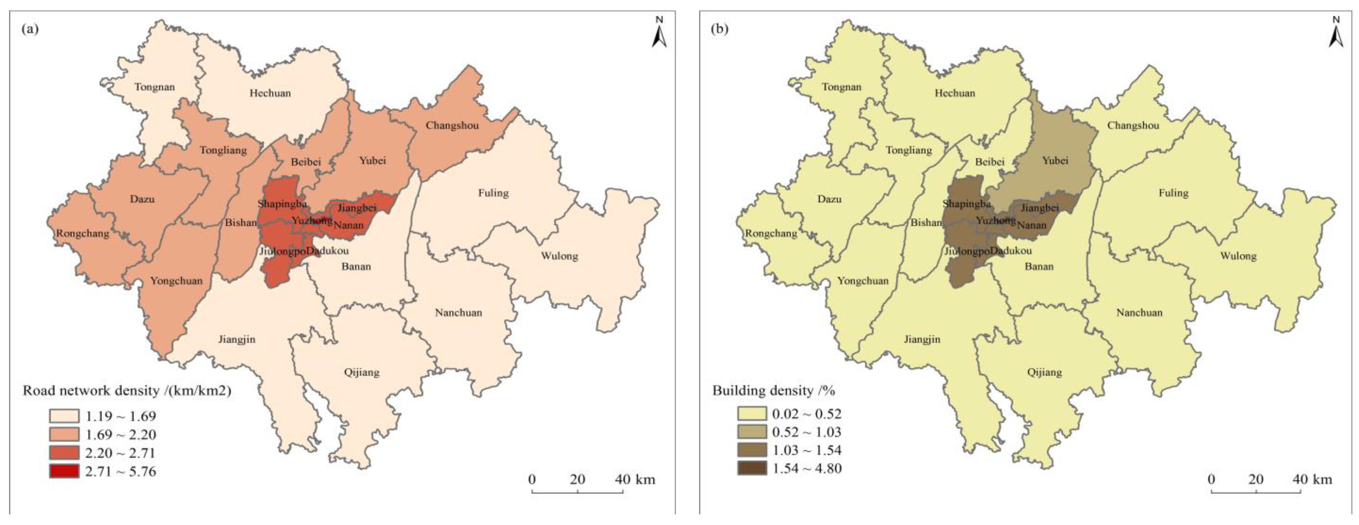
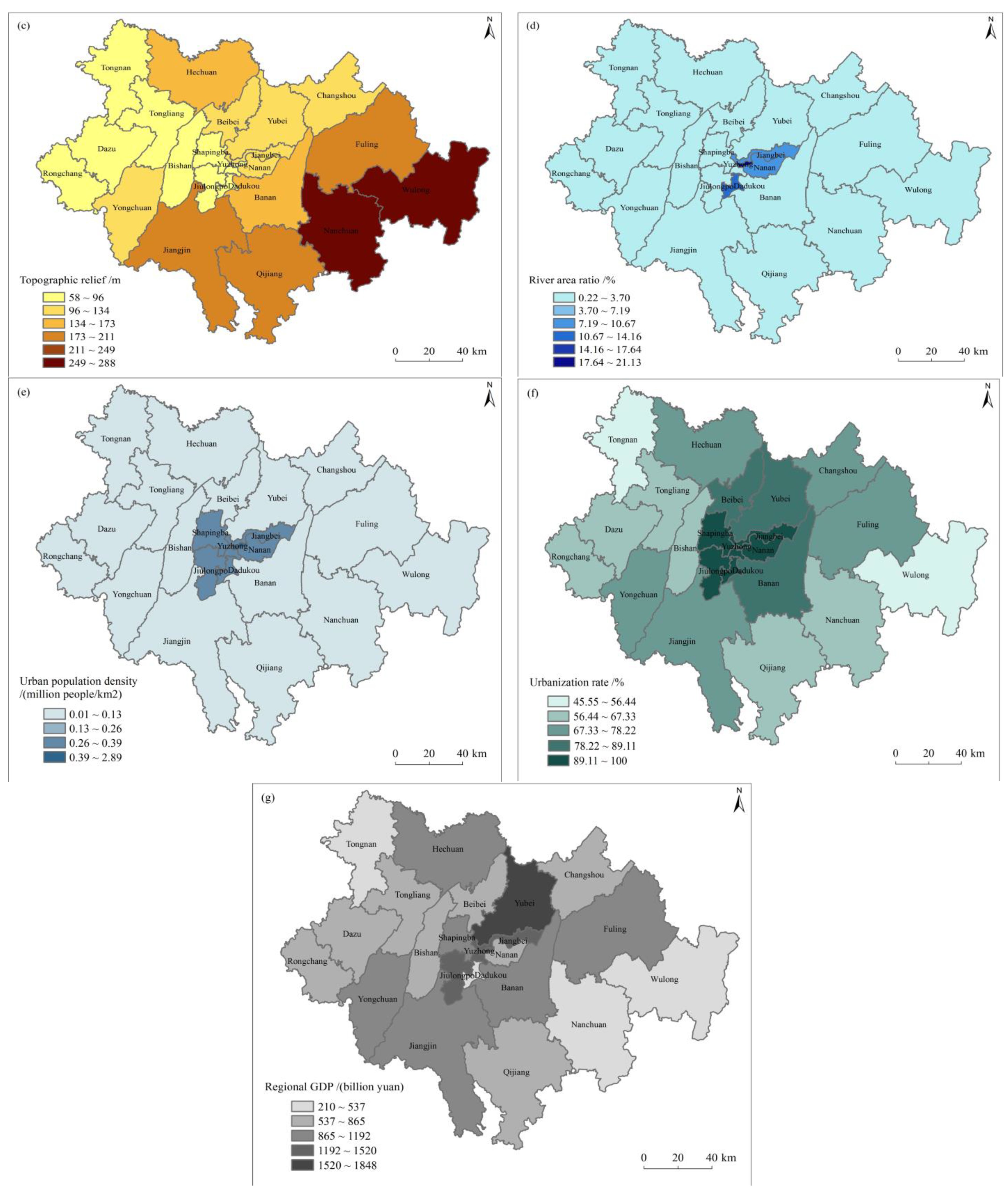
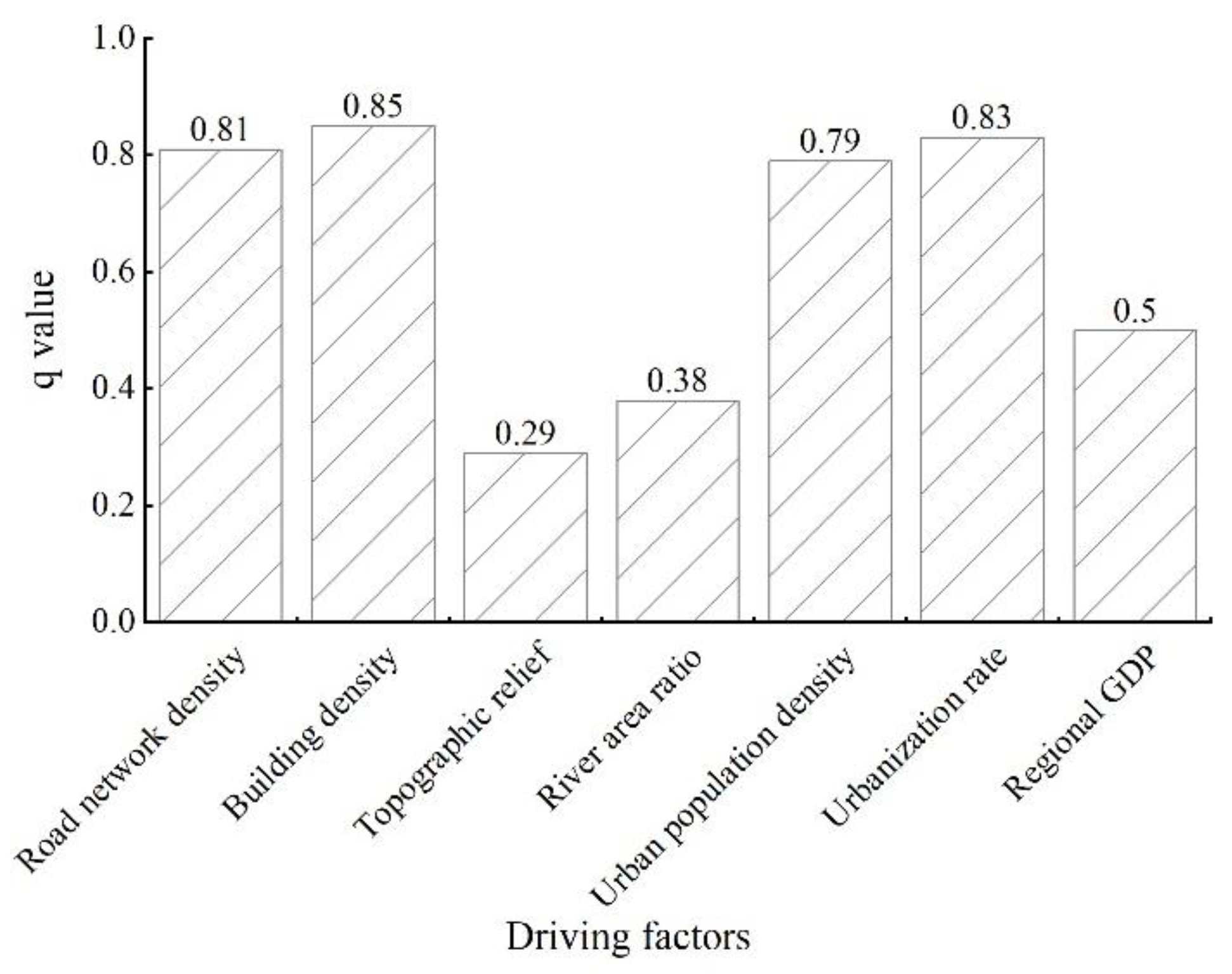
Based on the factor detection analysis, the compactness of urban spatial structure, the scale of a city and the flow of urban population had the greatest influence on the optimal distance threshold for identifying physical urban area, with the index value of influence degree ≥0.79. Among them, there was no significant difference in the influence of the four factors of road network density, building density, urban population density and urbanization rate on the optimal distance threshold. The regional GDP, river area ratio and topographic relief that had little influence on the optimal distance threshold also show insignificant difference. Based on the interaction detection analysis, the pairwise interaction of the three groups of driving factors was greater than the influence of a single factor on the optimal distance threshold. The interaction relationship between any two factors included nonlinear enhancement and bilinear enhancement. Where the synergistic effect of the compactness of urban spatial structure, the scale of a city and the flow of urban population with regional GDP of economic indicator had the most significant impact on the optimal distance threshold, the index value of influence degree is ≥0.93.

(3)

Under the synergistic influence of the 7 various factors, the explanatory power of the optimal distance threshold was greatly enhanced and the optimal distance threshold regularly corresponded to different stages of buffer radius in the process of expansion, which had the characteristics of self-adaptation. In addition to the Ba’nan district and the Beibei district, the optimal distance thresholds of the Chongqing central districts were between 100–1000 m, and the optimal distance threshold of peripheral districts were at the stage of 20–100 m.

References

1. Land Space Planning Bureau; Ministry of Natural Resources. Scientific Identification of Urban Areas to Enhance Spatial Governance Capacity; China Natural Resources News: Shenzhen, China, 2021; pp. 7–22. [Google Scholar]
2. Qi, W.; Wang, K.Y. Spatial differences and optimization integration between urban administrative areas and physical areas in China. Geogr. Res. 2019, 38, 207–220. [Google Scholar]
3. Zhou, Y.X.; Shi, Y.L. The concept of physical area for the establishment of Chinese cities. Acta Geogr. Sin. 1995, 4, 289–301. [Google Scholar]
4. Chen, X.X.; Feng, J. Discrimination and Research Progress of Urban Regional Concept. Urban Dev. Stud. 2020, 27, 62–69. [Google Scholar]
5. Kong, L.; He, Z.W.; Chen, Z.S.; Luo, M.L.; Du, Z.; Zhu, F.Q.; He, L. Spatial distribution and morphological identification of regional urban settlements based on road intersections. ISPRS Int. J. Geo-Inf. 2021, 10, 201. [Google Scholar] [CrossRef]
6. Department of the Ministry of Construction of the People’s Republic of China. Standards for Basic Terms of Urban Planning; China Construction Industry Press: Beijing, China, 1999. [Google Scholar]
7. Zhou, Y.X. Urban Geography; The commercial Press: Beijing, China, 1995. [Google Scholar]
8. Chen, Y.G. Fractal Urban System: Scale Symmetry Spatial Complexity; Science Press: Beijing, China, 2008. [Google Scholar]
9. Fang, C.L. Research progress and basic judgment of urban agglomeration spatial scope identification standard. Urban Plan. Forum 2009, 4, 6. [Google Scholar]
10. Rozenfeld, H.; Rybski, D.; Gabaix, X.; Makse, H. The area and population of cities: New insights from a different perspective on cities. Am. Econ. Rev. 2010, 101, 2205–2225. Available online: https://www.aeaweb.org/articles?id=10.1257/aer.101.5.2205 (accessed on 1 January 2021). [CrossRef] [Green Version]
11. Cao, F.J.; Qiu, Y.; Zou, Y. Fast extraction method of built-up area based on H/T fracture method and POI data. Geogr. Geo-Inf. Sci. 2020, 36, 7. [Google Scholar]
12. Zhang, H.C.; Ning, X.G.; Shao, Z.F.; Wang, H. Spatiotemporal pattern analysis of china’s cities based on high-resolution imagery from 2000 to 2015. ISPRS Int. J. Geo-Inf. 2019, 8, 241. [Google Scholar] [CrossRef] [Green Version]
13. Zhou, Y.; Tu, M.G.; Wang, S.X.; Liu, W.L. A novel approach for identifying urban built-up area boundaries using high-resolution remote-sensing data based on the scale effect. ISPRS Int. J. Geo-Inf. 2018, 7, 135. [Google Scholar] [CrossRef] [Green Version]
14. Ma, Y.T.; Xie, Z.W.; You, Y.C.; Xuan, X. Research on Rapid Extraction Method of Urban Built-Up Area with Multiple Remote Sensing Indexes. In Book Geoinformatics in Sustainable Ecosystem and Society; Springer: Guangzhou, China, 2020; pp. 199–209. [Google Scholar]
15. Xu, T.T.; Coco, G.; Gao, J. Extraction of urban built-up areas from nighttime lights using artificial neural network. Geocarto Int. 2018, 35, 1049–1066. [Google Scholar] [CrossRef]
16. Yu, B.L.; Tang, M.; Wu, Q.S.; Yang, C.S.; Deng, S.Q.; Shi, K.F.; Peng, C.; Wu, J.P.; Chen, Z.Q. Urban built-up area extraction from log-transformed NPP-VIIRS nighttime light composite data. IEEE Geosci. Remote Sens. Lett. 2018, 15, 1279–1283. Available online: https://ieeexplore.ieee.org/document/8358755 (accessed on 1 January 2021). [CrossRef]
17. Su, Y.X.; Chen, X.Z.; Wang, C.Y.; Zhang, H.O.; Liao, J.S.; Ye, Y.Y. A new method for extracting built-up urban areas using DMSP-OLS nighttime stable lights: A case study in the pearl river delta, southern china. Giscience Remote Sens. 2015, 52, 218–238. [Google Scholar] [CrossRef]
18. Lin, X.J.; Fang, S.F.; Xu, Y.L.; Zou, B.Y.; Luo, M.L. Urban Boundary Identification Based on Neighborhood Expansion Curve of Road Intersection Points—Taking Chengdu, Xi’an, Wuhan, Nanjing and Changsha as Examples. Prog. Geogr. 2018, 37, 781–789. [Google Scholar]
19. Jiang, B.; Jia, T. Zipf’s law for all the natural cities in the united states: A geospatial perspective. Int. J. Geogr. Inf. Sci. 2011, 25, 1269–1281. [Google Scholar] [CrossRef]
20. Jia, T.; Jiang, B. Measuring Urban Sprawl Based on Massive Street Nodes and the Novel Concept of Natural Cities. Physics 2012. Available online: https://arxiv.org/abs/1010.0541 (accessed on 1 November 2021).
21. Jiang, B. Natural cities generated from all building locations in America. Data 2019, 4, 59. [Google Scholar] [CrossRef] [Green Version]
22. Tannier, C.; Thomas, I.; Vuidel, G.; Frankhauser, P. A fractal approach to identifying urban boundaries. Geogr. Anal. 2011, 43, 211–227. [Google Scholar] [CrossRef]
23. Tannier, C.; Thomas, I. Defining and characterizing urban boundaries: A fractal analysis of theoretical cities and Belgian cities. Comput. Environ. Urban Syst. 2013, 41, 234–248. [Google Scholar] [CrossRef]
24. Chen, Y.G. How high is urbanization in China? Why do urban geography research draw on fractal geometry? City Plan. Review 2003, 7, 12–17. [Google Scholar]
25. Chen, Y.G.; Wang, J.J. Multifractal characterization of urban form and growth: The case of Beijing. Environ. Plan. B Urban Anal. City Sci. 2013, 40, 884–904. [Google Scholar] [CrossRef]
26. Ogoke, U. Correlational analysis of someinfectious diseases. IOSR J. Math. 2022, 14, 54–57. [Google Scholar]
27. Zhou, Y.; Zhao, C. Research on government subsidy, internal control and overinvestment in enterprises by multiple regression analysis method: Based on multiple regression analysis method. In Proceedings of the Management Science Informatization and Economic Innovation Development Conference, Guangzhou, China, 18–20 December 2020; pp. 285–288. [Google Scholar]
28. Yu, G. The influencing factors of drug addiction based on principal component analysis model. IOP Conf. Ser. Mater. Sci. Eng. 2019, 612, 022002. [Google Scholar] [CrossRef]
29. Wang, J.F.; Xu, C.D. Geodetector: Principle and prospect. Acta Geogr. Sin. 2017, 72, 116–134. [Google Scholar]
30. Ahmadpoor, N.; Smith, A.D.; Heath, T. Rethinking legibility in the era of digital mobile maps: An empirical study. J. Urban Des. 2020, 26, 296–318. [Google Scholar] [CrossRef]
31. Jokar Arsanjani, J.; Mooney, P.; Zipf, A.; Helbich, M. OpenStreetMap in GIScience: Experiences, Research, Applications; Springer: New York, NY, USA, 2015. [Google Scholar]
32. Mandelbrot, B.B. The fractal geometry on nature. Am. J. Phys. 1983, 51, 468. [Google Scholar] [CrossRef]
33. Minkowski, H. Volumen und Oberfläche. Math. Ann. 1903, 57, 447–495. [Google Scholar] [CrossRef] [Green Version]
34. Lowe, D.G. Organization of smooth image curves at multiple scales. Int. J. Comput. Vis. 1988, 3, 119–130. [Google Scholar] [CrossRef]
35. Huang, J.X.; Wang, J.F.; Bo, Y.C.; Xu, C.D.; Hu, M.G.; Huang, D.C. Identification of health risks of hand, foot and mouth disease in china using the geographical detector technique. Int. J. Environ. Res. Public Health 2014, 11, 3407–3423. [Google Scholar] [CrossRef]
36. Tung Chi University; Xi’an University of Architecture and Technology; Southeast University; Chongqing University. Fourth Edition of Housing Architecture; China Construction Industry Press: Beijing, China, 2005. [Google Scholar]
37. Shi, F.; Yin, H.W. Research on Dynamic Optimization Method of Urban Road Grade Structure. In Book Annual Meeting of Asian Transportation Society and ‘Transportation and Logistics’ Symposium; Science and Technology of China Press: Dalian, China, 2007. [Google Scholar]
38. Huang, X.; Li, J.Y.; Jie, Y.; Zhang, Z.; Li, D.R.; Liu, X.P. 30 m global impervious surface area dynamics and urban expansion pattern observed by landsat satellites: From 1972 to 2019. Sci. China Earth Sci. 2021, 64, 1922–1933. Available online: https://link.springer.com/article/10.1007/s11430-020-9797-9 (accessed on 1 December 2021). [CrossRef]
39. Zhao, M.; Cheng, C.X.; Zhou, Y.Y.; Li, X.C.; Shen, S.; Song, C.Q. A global dataset of annual urban extents (1992–2020) from harmonized nighttime lights. Earth Syst. Sci. Data 2022, 14, 517–534. Available online: https://essd.copernicus.org/articles/14/517/2022/ (accessed on 1 October 2022). [CrossRef]
40. Portugali, J. Self-organizing cities. Futures 1997, 29, 353–380. [Google Scholar] [CrossRef]
41. Portugali, J. Self-Organization and the City; Springer: New York, NY, USA, 1999. [Google Scholar]
42. Wu, K.H.; Li, C.K.; Liu, J.J.; Hao, H.J. Development boundary identification of urban agglomeration core area based on spatial syntax theory. Geogr. Res. 2020, 39, 1418–1426. [Google Scholar]
43. Zhan, D.S.; Zhang, W.Z.; Yu, J.H.; Meng, B.; Dang, Y.X. The impact mechanism of Beijing residents’ livable satisfaction based on geographical detectors. Prog. Geogr. 2015, 34, 966–975. [Google Scholar]
44. Li, J. Urban Design Theory and Method; Wuhan University Press: Wuhan, China, 2010. [Google Scholar]
45. Tan, X.Y.; Huang, B. Identifying urban agglomerations in china based on density—Density correlation functions. Ann. Am. Assoc. Geogr. 2022, 112, 1666–1684. [Google Scholar] [CrossRef]
46. Long, H.L.; Wu, X.Q.; Wang, W.J.; Dong, G.H. Analysis of urban-rural land-use change during 1995–2006 and its policy dimensional driving forces in Chongqing, china. Sensors 2008, 8, 681–699. [Google Scholar] [CrossRef] [PubMed] [Green Version]
47. Li, D.H. Third Edition of Urban Planning Principle; China Construction Industry Press: Beijing, China, 2001. [Google Scholar]
48. Wu, Z.Q.; Li, D.H. Urban Planning Principle; China Construction Industry Press: Beijing, China, 2010. [Google Scholar]
49. Liang, L.; Chen, M.; Lu, D. Revisiting the relationship between urbanization and economic development in china since the reform and opening-up. Chin. Geogr. Sci. 2022, 32, 1–15. Available online: https://link.springer.com/article/10.1007/s11769-022-1255-7 (accessed on 1 October 2022). [CrossRef]
Figure 1. Research area.
Land 12 00030 g001
Figure 2. Partial vector building data (a) and partial road intersection data extracted from road network (b).
Land 12 00030 g002
Figure 3. Spatial distribution of 7 driving factors for partition.
Land 12 00030 g003aLand 12 00030 g003b
Figure 4. Physical urban area based on vector building data.
Land 12 00030 g004
Figure 5. Factor detection results.
Land 12 00030 g005
Figure 6. Physical urban area comparison between different types of data and vector building data.
Land 12 00030 g006aLand 12 00030 g006b