

Machine Learning Models for Prediction of Soil Properties in the Riparian Forests

 ,
, 

Abstract
:1. Introduction
2. Materials and Methods
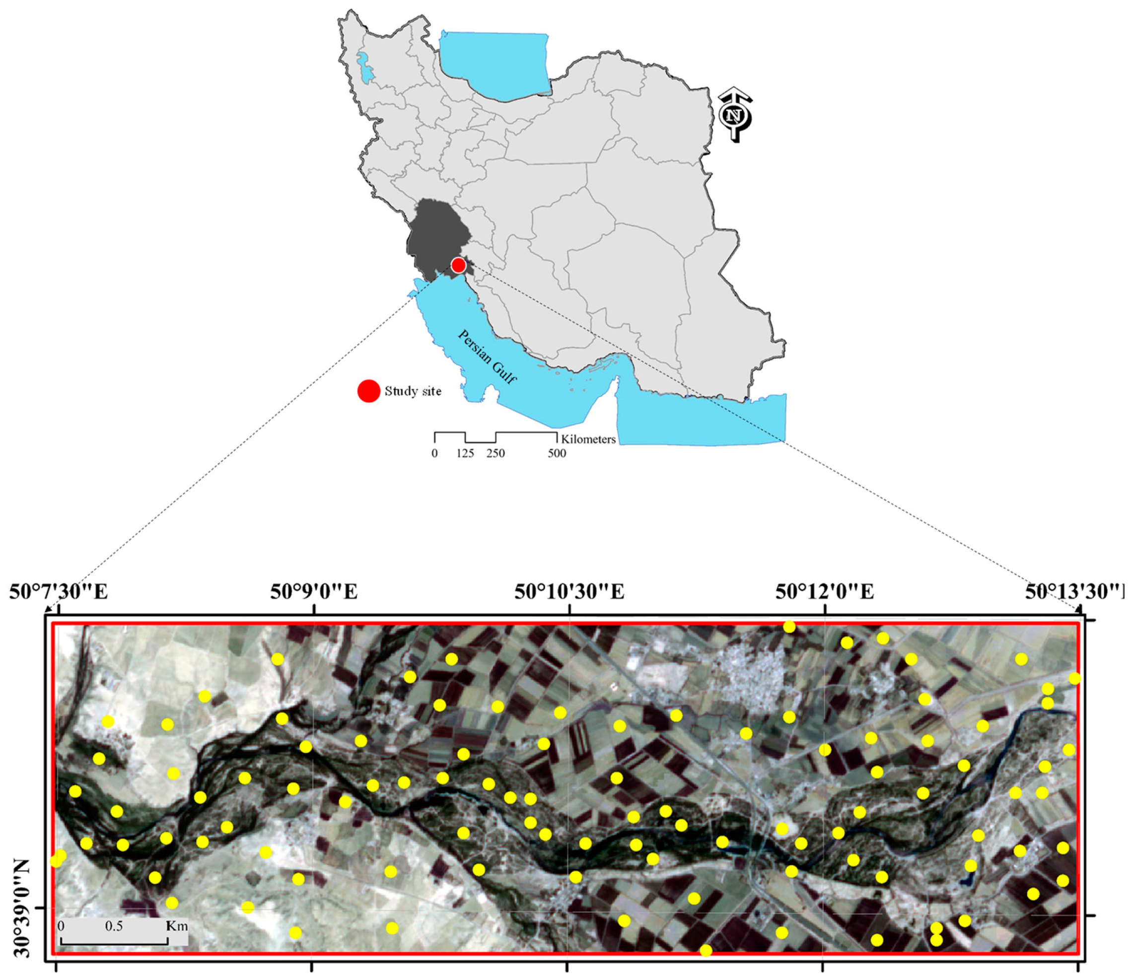
2.1. Study Site
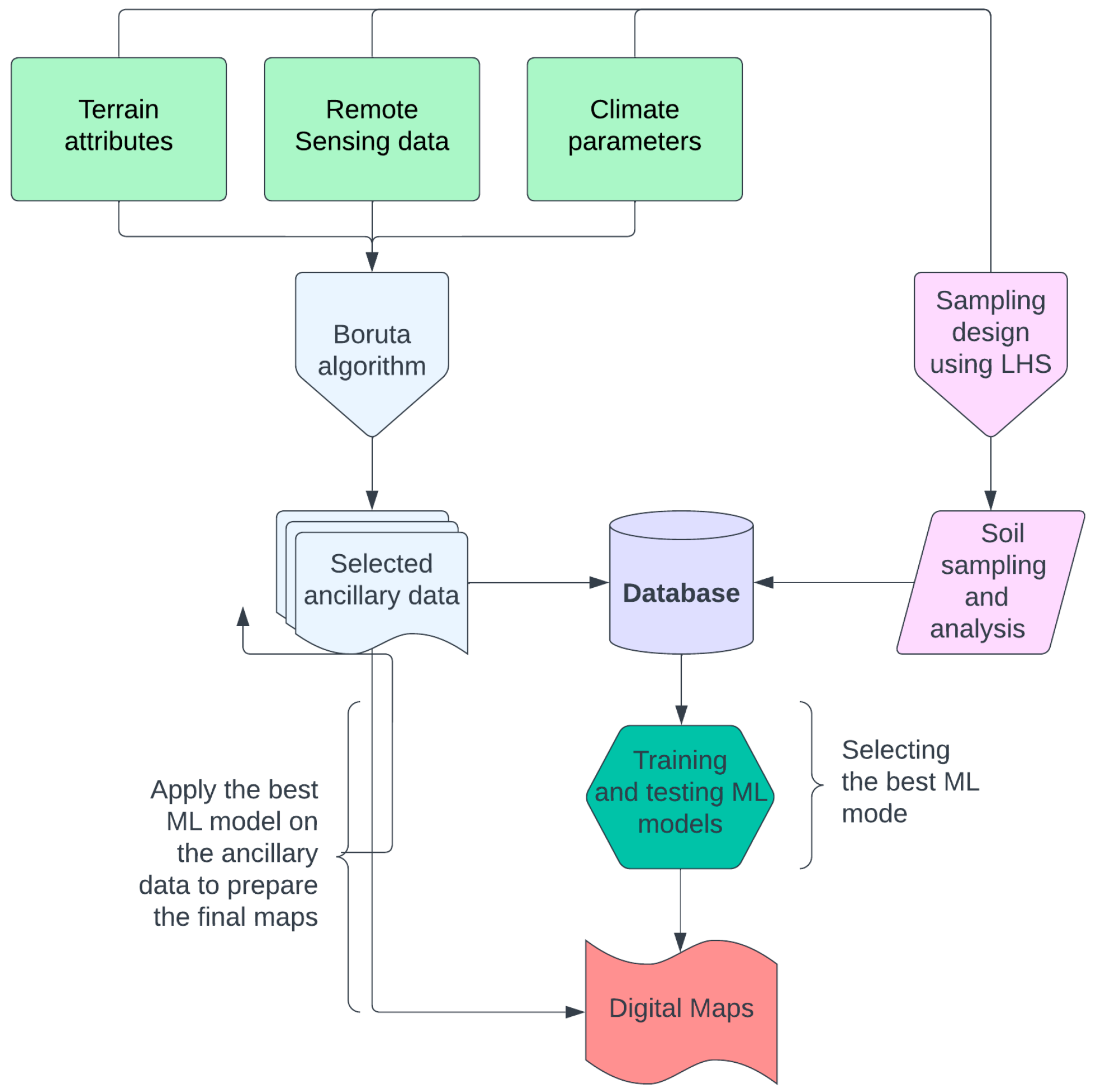
2.2. Procedures
2.3. Soil Data Sampling and Analysis
2.4. Ancillary Data
2.5. Machine Learning Models
3. Results and Discussion
3.1. Summary of Soil Properties
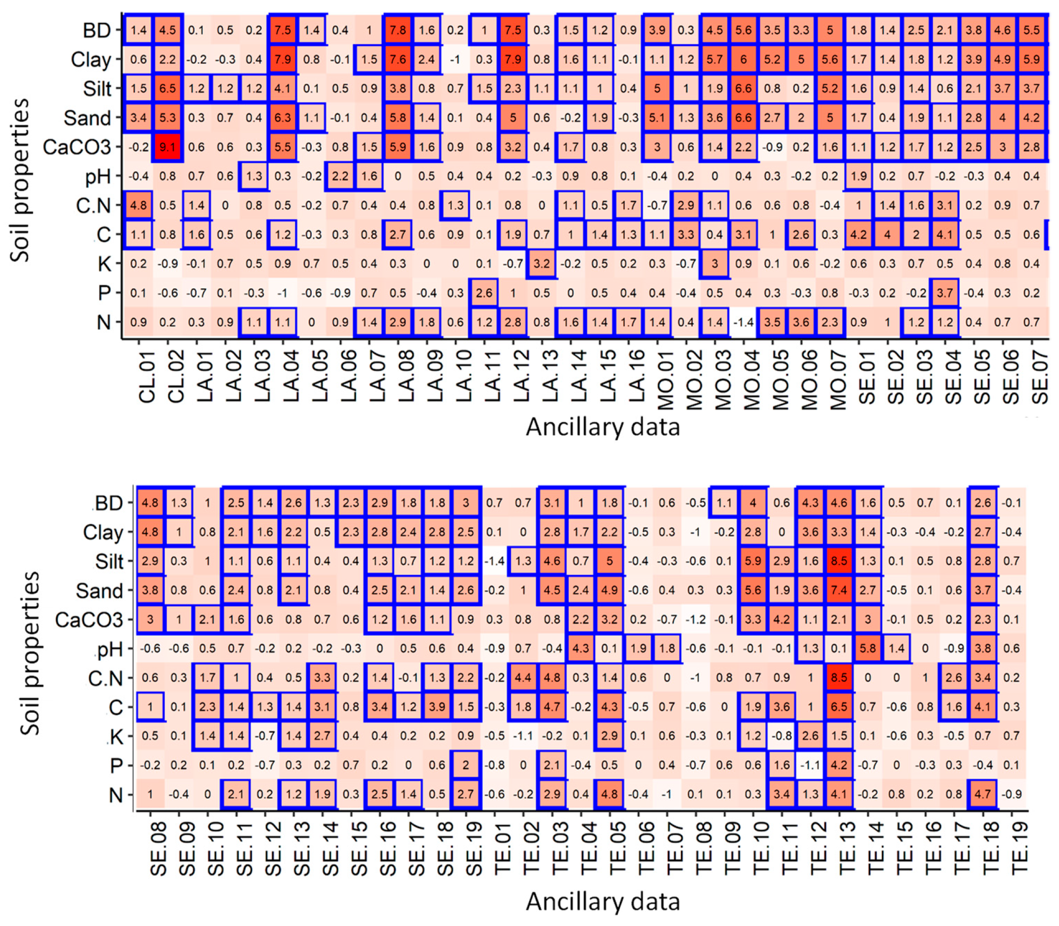
3.2. Importance of Ancillary Data
3.3. Machine Learning Performances
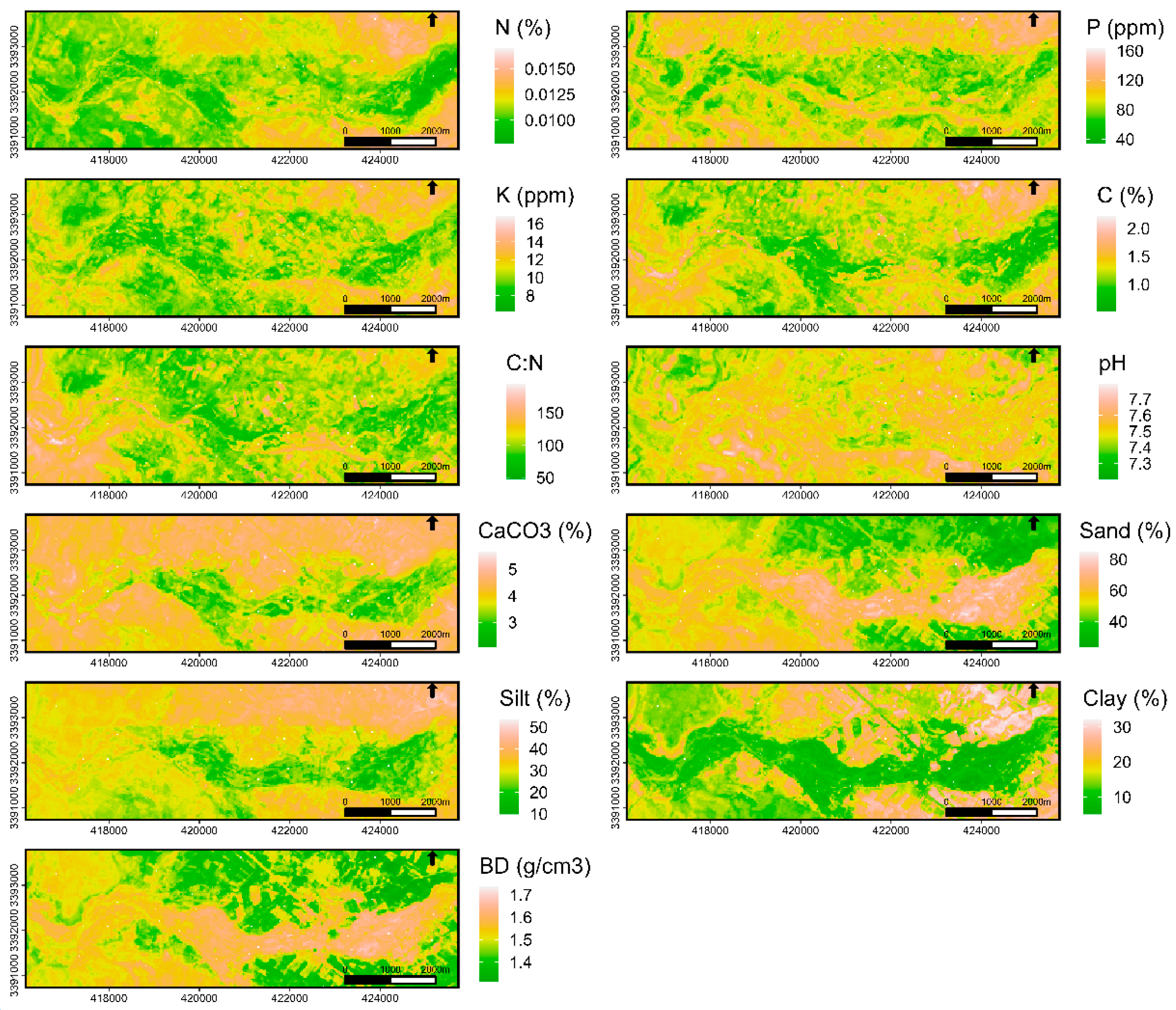
3.4. Spatial Pattern of Maps
4. Conclusions
Author Contributions
Funding
Data Availability Statement
Acknowledgments
Conflicts of Interest
References
- Muñoz-Rojas, M.; Erickson, T.E.; Martini, D.; Dixon, K.W.; Merritt, D.J. Soil Physicochemical and Microbiological Indicators of Short, Medium and Long Term Post-Fire Recovery in Semi-Arid Ecosystems. Ecol. Indic. 2016, 63, 14–22. [Google Scholar] [CrossRef]
- Visschers, R.; Finke, P.A.; de Gruijter, J.J. A Soil Sampling Program for the Netherlands. Geoderma 2007, 139, 60–72. [Google Scholar] [CrossRef] [Green Version]
- Lamsal, S.; Bliss, C.M.; Graetz, D.A. Geospatial Mapping of Soil Nitrate-Nitrogen Distribution Under a Mixed-Land Use System. Pedosphere 2009, 19, 434–445. [Google Scholar] [CrossRef]
- Klemas, V. Remote Sensing of Riparian and Wetland Buffers: An Overview. J. Coast. Res. 2014, 297, 869–880. [Google Scholar] [CrossRef] [Green Version]
- McBratney, A.B.; Mendonça Santos, M.L.; Minasny, B. On Digital Soil Mapping. Geoderma 2003, 117, 3–52. [Google Scholar] [CrossRef]
- Hengl, T.; Toomanian, N.; Reuter, H.I.; Malakouti, M.J. Methods to Interpolate Soil Categorical Variables from Profile Observations: Lessons from Iran. Geoderma 2007, 140, 417–427. [Google Scholar] [CrossRef]
- Gundogdu, I.B.; Esen, O. The importance of secondary variables for mapping of meteorological data. In Proceedings of the International Conference on Cartography and GIS, Nessebar, Bulgaria, 15–20 June 2010. [Google Scholar]
- Ließ, M.; Schmidt, J.; Glaser, B. Improving the Spatial Prediction of Soil Organic Carbon Stocks in a Complex Tropical Mountain Landscape by Methodological Specifications in Machine Learning Approaches. PLoS ONE 2016, 11, e0153673. [Google Scholar] [CrossRef] [Green Version]
- Were, K.; Bui, D.T.; Dick, Ø.B.; Singh, B.R. A Comparative Assessment of Support Vector Regression, Artificial Neural Networks, and Random Forests for Predicting and Mapping Soil Organic Carbon Stocks across an Afromontane Landscape. Ecol. Indic. 2015, 52, 394–403. [Google Scholar] [CrossRef]
- Viscarra Rossel, R.A.; Behrens, T. Using Data Mining to Model and Interpret Soil Diffuse Reflectance Spectra. Geoderma 2010, 158, 46–54. [Google Scholar] [CrossRef]
- Hardoim, P.R.; van Overbeek, L.S.; Berg, G.; Pirttilä, A.M.; Compant, S.; Campisano, A.; Döring, M.; Sessitsch, A. The Hidden World within Plants: Ecological and Evolutionary Considerations for Defining Functioning of Microbial Endophytes. Microbiol. Mol. Biol. Rev. 2015, 79, 293–320. [Google Scholar] [CrossRef]
- Štursová, M.; Bárta, J.; Šantrůčková, H.; Baldrian, P. Small-Scale Spatial Heterogeneity of Ecosystem Properties, Microbial Community Composition and Microbial Activities in a Temperate Mountain Forest Soil. FEMS Microbiol. Ecol. 2016, 92, fiw185. [Google Scholar] [CrossRef] [PubMed] [Green Version]
- Ingole, S.P. A Review on Role of Physico-Chemical Properties in Soil Quality. Int. J. Chem. Stud. 2015, 3, 29–32. [Google Scholar]
- Moradi Behbahani, S.; Moradi, M.; Basiri, R.; Mirzaei, J. Sand Mining Disturbances and Their Effects on the Diversity of Arbuscular Mycorrhizal Fungi in a Riparian Forest of Iran. J. Arid Land 2017, 9, 837–849. [Google Scholar] [CrossRef] [Green Version]
- Moradi, M.; Imani, F.; Naji, H.; Moradi Behbahani, S.; Ahmadi, M. Variation in Soil Carbon Stock and Nutrient Content in Sand Dunes after Afforestation by Prosopis Juliflora in the Khuzestan Province (Iran). iForest 2017, 10, 585–589. [Google Scholar] [CrossRef] [Green Version]
- Narumalani, S.; Zhou, Y.; Jensen, J.R. Application of Remote Sensing and Geographic Information Systems to the Delineation and Analysis of Riparian Buffer Zones. Aquat. Bot. 1997, 58, 393–409. [Google Scholar] [CrossRef]
- Alencar-Silva, T.; Maillard, P. Assessment of biophysical structure of riparian zones based on segmentation method, spatial knowledge and texture analysis. In ISPRS TC VII Symposium—100 Years ISPRS; Wagner, W., Szekely, B., Eds.; IAPRS: Vienna, Austria, 2010. [Google Scholar]
- Forogh Nasab, F.; Moradi, M.; Moradi, G.; Taghizadeh-Mehrjardi, R. Erratum to: Topsoil Carbon Stock and Soil Physicochemical Properties in Riparian Forests and Agricultural Lands of Southwestern Iran. Eurasian Soil Sci. 2021, 54, 459. [Google Scholar] [CrossRef]
- Avazpoor, Z.; Moradi, M.; Basiri, R.; Mirzaei, J.; Taghizadeh-Mehrjardi, R.; Kerry, R. Soil Enzyme Activity Variations in Riparian Forests in Relation to Plant Species and Soil Depth. Arab. J. Geosci. 2019, 12, 708. [Google Scholar] [CrossRef]
- Tockner, K.; Stanford, J.A. Riverine Flood Plains: Present State and Future Trends. Environ. Conserv. 2002, 29, 308–330. [Google Scholar] [CrossRef] [Green Version]
- Rusnák, M.; Goga, T.; Michaleje, L.; Šulc Michalková, M.; Máčka, Z.; Bertalan, L.; Kidová, A. Remote Sensing of Riparian Ecosystems. Remote Sens. 2022, 14, 2645. [Google Scholar] [CrossRef]
- Minasny, B.; McBratney, A.B. Chapter 12 Latin Hypercube Sampling as a Tool for Digital Soil Mapping. In Developments in Soil Science; Elsevier: Amsterdam, The Netherlands, 2006; Volume 31, pp. 153–606. ISBN 9780444529589. [Google Scholar]
- Mclean, E.O. Soil PH and Lime Requirement. In Agronomy Monographs; Page, A.L., Ed.; American Society of Agronomy, Soil Science Society of America: Madison, WI, USA, 2015; pp. 199–224. ISBN 9780891189770. [Google Scholar]
- Walkley, A.; Black, I.A. An examination of the degtjareff method for determining soil organic matter, and a proposed modification of the chromic acid titration method. Soil Sci. 1934, 37, 29–38. [Google Scholar] [CrossRef]
- Klute, A.; Page, A.L. (Eds.) Methods of Soil Analysis, 2nd ed.; Agronomy; American Society of Agronomy, Soil Science Society of America: Madison, WI, USA, 1982; ISBN 9780891180883. [Google Scholar]
- Olsen, S.R.; Cole, C.V.; Watanabe, F.S.; Dean, L.A. Estimation of available phosphorus in soils by extraction with sodium bicarbonate. USDA Circ. 1954, 939, 1–19. [Google Scholar]
- Merwin, H.D.; Peech, M. Exchangeability of Soil Potassium in the Sand, Silt, and Clay Fractions as Influenced by the Nature of the Complementary Exchangeable Cation. Soil Sci. Soc. Am. J. 1951, 15, 125–128. [Google Scholar] [CrossRef]
- Prihar, S.S.; Hundal, S.S. Determination of Bulk Density of Soil Clod by Saturation. Geoderma 1971, 5, 283–286. [Google Scholar] [CrossRef]
- Loveland, T.R.; Irons, J.R. Landsat 8: The Plans, the Reality, and the Legacy. Remote Sens. Environ. 2016, 185, 1–6. [Google Scholar] [CrossRef] [Green Version]
- Conrad, O.; Bechtel, B.; Bock, M.; Dietrich, H.; Fischer, E.; Gerlitz, L.; Wehberg, J.; Wichmann, V.; Böhner, J. System for Automated Geoscientific Analyses (SAGA) v. 2.1.4. Geosci. Model Dev. 2015, 8, 1991–2007. [Google Scholar] [CrossRef] [Green Version]
- Hijmans, R.; Cameron, S.; Parra, J.; Jones, P.; Jarvis, A.; Richardson, K. Very high resolution interpolated climate surfaces for global land areas. Int. J. Climatol. A J. R. Meteorol. Soc. 2005, 25, 1965–1978. [Google Scholar] [CrossRef]
- Kursa, M.B.; Jankowski, A.; Rudnicki, W.R. Boruta—A System for Feature Selection. Fundam. Inform. 2010, 101, 271–285. [Google Scholar] [CrossRef]
- Bittencourt, H.R.; Clarke, R.T. Use of Classification and Regression Trees (CART) to Classify Remotely-Sensed Digital Images. In Proceedings of the IGARSS 2003, 2003 IEEE International Geoscience and Remote Sensing Symposium, Toulouse, France, 21–25 July 2003; Proceedings (IEEE Cat. No.03CH37477). IEEE: Toulouse, France, 2003; Volume 6, pp. 3751–3753. [Google Scholar]
- Taghizadeh-Mehrjardi, R.; Sarmadian, F.; Omid, M.; Toomanian, N.; Rousta, M.J.; Rahimian, M.H. Incorporating soil taxonomic distance and decision tree for spatial prediction of soil classes in Ardakan, Yazd. J. Arid Biome 2013, 3, 27–39. [Google Scholar]
- Cutler, D.R.; Edwards, T.C.; Beard, K.H.; Cutler, A.; Hess, K.T.; Gibson, J.; Lawler, J.J. Random forests for classification in ecology. Ecology 2007, 88, 2783–2792. [Google Scholar] [CrossRef]
- Dramsch, J.S. 70 Years of Machine Learning in Geoscience in Review. In Advances in Geophysics; Elsevier: Amsterdam, The Netherlands, 2020; Volume 61, pp. 1–55. ISBN 9780128216699. [Google Scholar]
- Behrens, T.; Förster, H.; Scholten, T.; Steinrücken, U.; Spies, E.; Goldschmitt, M. Digital Soil Mapping Using Artificial Neural Networks. Z. Pflanz. Bodenkd. 2005, 168, 21–33. [Google Scholar] [CrossRef]
- Kalambukattu, J.G.; Kumar, S.; Arya Raj, R. Digital Soil Mapping in a Himalayan Watershed Using Remote Sensing and Terrain Parameters Employing Artificial Neural Network Model. Environ. Earth Sci. 2018, 77, 203. [Google Scholar] [CrossRef]
- Quinlan, R. Learning with Continuous Classes. In Proceedings of the 5th Australian Joint Conference on Artificial Intelligence, Hobart, Tasmania, 16–18 November 1992; pp. 343–348. [Google Scholar]
- Appelhans, T.; Mwangomo, E.; Hardy, D.R.; Hemp, A.; Nauss, T. Evaluating Machine Learning Approaches for the Interpolation of Monthly Air Temperature at Mt. Kilimanjaro, Tanzania. Spat. Stat. 2015, 14, 91–113. [Google Scholar] [CrossRef] [Green Version]
- Emadi, M.; Taghizadeh-Mehrjardi, R.; Cherati, A.; Danesh, M.; Mosavi, A.; Scholten, T. Predicting and Mapping of Soil Organic Carbon Using Machine Learning Algorithms in Northern Iran. Remote Sens. 2020, 12, 2234. [Google Scholar] [CrossRef]
- Sun, H.; Wang, Q.; Wang, G.; Lin, H.; Luo, P.; Li, J.; Zeng, S.; Xu, X.; Ren, L. Optimizing KNN for Mapping Vegetation Cover of Arid and Semi-Arid Areas Using Landsat Images. Remote Sens. 2018, 10, 1248. [Google Scholar] [CrossRef] [Green Version]
- Mansuy, N.; Thiffault, E.; Paré, D.; Bernier, P.; Guindon, L.; Villemaire, P.; Poirier, V.; Beaudoin, A. Digital Mapping of Soil Properties in Canadian Managed Forests at 250 m of Resolution Using the K-Nearest Neighbor Method. Geoderma 2014, 235–236, 59–73. [Google Scholar] [CrossRef]
- Taghizadeh-Mehrjardi, R.; Emadi, M.; Cherati, A.; Heung, B.; Mosavi, A.; Scholten, T. Bio-Inspired Hybridization of Artificial Neural Networks: An Application for Mapping the Spatial Distribution of Soil Texture Fractions. Remote Sens. 2021, 13, 1025. [Google Scholar] [CrossRef]
- Mirzaeitalarposhti, R.; Shafizadeh-Moghadam, H.; Taghizadeh-Mehrjardi, R.; Demyan, M.S. Digital Soil Texture Mapping and Spatial Transferability of Machine Learning Models Using Sentinel-1, Sentinel-2, and Terrain-Derived Covariates. Remote Sens. 2022, 14, 5909. [Google Scholar] [CrossRef]
- Taghizadeh-Mehrjardi, R.; Khademi, H.; Khayamim, F.; Zeraatpisheh, M.; Heung, B.; Scholten, T. A Comparison of Model Averaging Techniques to Predict the Spatial Distribution of Soil Properties. Remote Sens. 2022, 14, 472. [Google Scholar] [CrossRef]
- Mahmoudzadeh, H.; Matinfar, H.R.; Kerry, R.; Eskandari, S.; Ebrahimi-Khusfi, Z.; Taghizadeh-Mehrjardi, R. New Hybrid Evolutionary Models for Spatial Prediction of Soil Properties in Kurdistan. Soil Use Manag. 2022, 38, 191–211. [Google Scholar] [CrossRef]
- Mahmoudzadeh, H.; Matinfar, H.R.; Taghizadeh-Mehrjardi, R.; Kerry, R. Spatial Prediction of Soil Organic Carbon Using Machine Learning Techniques in Western Iran. Geoderma Reg. 2020, 21, e00260. [Google Scholar] [CrossRef]
- Zeraatpisheh, M.; Garosi, Y.; Reza Owliaie, H.; Ayoubi, S.; Taghizadeh-Mehrjardi, R.; Scholten, T.; Xu, M. Improving the Spatial Prediction of Soil Organic Carbon Using Environmental Covariates Selection: A Comparison of a Group of Environmental Covariates. CATENA 2022, 208, 105723. [Google Scholar] [CrossRef]
- Zhao, X.; Yang, Y.; Shen, H.; Geng, X.; Fang, J. Global Soil–Climate–Biome Diagram: Linking Surface Soil Properties to Climate and Biota. Biogeosciences 2019, 16, 2857–2871. [Google Scholar] [CrossRef] [Green Version]
- Ding, J.; Li, F.; Yang, G.; Chen, L.; Zhang, B.; Liu, L.; Fang, K.; Qin, S.; Chen, Y.; Peng, Y.; et al. The Permafrost Carbon Inventory on the Tibetan Plateau: A New Evaluation Using Deep Sediment Cores. Glob. Chang. Biol. 2016, 22, 2688–2701. [Google Scholar] [CrossRef] [PubMed]
- Hengl, T.; Heuvelink, G.B.M.; Kempen, B.; Leenaars, J.G.B.; Walsh, M.G.; Shepherd, K.D.; Sila, A.; MacMillan, R.A.; Mendes de Jesus, J.; Tamene, L.; et al. Mapping Soil Properties of Africa at 250 m Resolution: Random Forests Significantly Improve Current Predictions. PLoS ONE 2015, 10, e0125814. [Google Scholar] [CrossRef] [PubMed]
- Dangal, S.R.S.; Sanderman, J.; Wills, S.; Ramirez-Lopez, L. Accurate and Precise Prediction of Soil Properties from a Large Mid-Infrared Spectral Library. Soil Syst. 2019, 3, 11. [Google Scholar] [CrossRef] [Green Version]
- Silva, S.H.G.; Teixeira, A.F.d.S.; Menezes, M.D.d.; Guilherme, L.R.G.; Moreira, F.M.d.S.; Curi, N. Multiple Linear Regression and Random Forest to Predict and Map Soil Properties Using Data from Portable X-ray Fluorescence Spectrometer (PXRF). Ciênc. Agrotechnol. 2017, 41, 648–664. [Google Scholar] [CrossRef]
- Adhikari, K.; Owens, P.R.; Libohova, Z.; Miller, D.M.; Wills, S.A.; Nemecek, J. Assessing Soil Organic Carbon Stock of Wisconsin, USA and Its Fate under Future Land Use and Climate Change. Sci. Total Environ. 2019, 667, 833–845. [Google Scholar] [CrossRef]
- Zeraatpisheh, M.; Ayoubi, S.; Jafari, A.; Tajik, S.; Finke, P. Digital Mapping of Soil Properties Using Multiple Machine Learning in a Semi-Arid Region, Central Iran. Geoderma 2019, 338, 445–452. [Google Scholar] [CrossRef]
- Taghizadeh-Mehrjardi, R.; Schmidt, K.; Amirian-Chakan, A.; Rentschler, T.; Zeraatpisheh, M.; Sarmadian, F.; Valavi, R.; Davatgar, N.; Behrens, T.; Scholten, T. Improving the Spatial Prediction of Soil Organic Carbon Content in Two Contrasting Climatic Regions by Stacking Machine Learning Models and Rescanning Covariate Space. Remote Sens. 2020, 12, 1095. [Google Scholar] [CrossRef] [Green Version]
- Taghizadeh-mehrjardi, R.; Toomanian, N.; Khavaninzadeh, A.R.; Jafari, A.; Triantafilis, J. Predicting and Mapping of Soil Particle-Size Fractions with Adaptive Neuro-Fuzzy Inference and Ant Colony Optimization in Central Iran: Digital Mapping of Soil Texture. Eur. J. Soil Sci. 2016, 67, 707–725. [Google Scholar] [CrossRef]
- Moline, A.B.; Poff, N.L. Growth of an Invertebrate Shredder on Native (Populus) and Non-Native (Tamarix, Elaeagnus) Leaf Litter. Freshw. Biol. 2008, 53, 1012–1020. [Google Scholar] [CrossRef]
- Vendramini, J.M.B.; Silveira, M.L.A.; Dubeux, J.C.B., Jr.; Sollenberger, L.E. Environmental Impacts and Nutrient Recycling on Pastures Grazed by Cattle. R. Bras. Zootec. 2007, 36, 139–149. [Google Scholar] [CrossRef]
- Crooks, E.C.; Harris, I.M.; Patil, S.D. Influence of Land Use Land Cover on River Water Quality in Rural North Wales, UK. J. Am. Water Resour. Assoc. 2021, 57, 357–373. [Google Scholar] [CrossRef]
- Fones, G.R.; Bakir, A.; Gray, J.; Mattingley, L.; Measham, N.; Knight, P.; Bowes, M.J.; Greenwood, R.; Mills, G.A. Using High-Frequency Phosphorus Monitoring for Water Quality Management: A Case Study of the Upper River Itchen, UK. Environ. Monit. Assess. 2020, 192, 184. [Google Scholar] [CrossRef] [PubMed] [Green Version]
- Günal, H.; Korucu, T.; Birkas, M.; Özgöz, E.; Halbac-Cotoara-Zamfir, R. Threats to Sustainability of Soil Functions in Central and Southeast Europe. Sustainability 2015, 7, 2161–2188. [Google Scholar] [CrossRef] [Green Version]
- Yang, L.; Chen, S.; Li, Y.; Wang, Q.; Zhong, X.; Yang, Z.; Lin, C.; Yang, Y. Conversion of Natural Evergreen Broadleaved Forests Decreases Soil Organic Carbon but Increases the Relative Contribution of Microbial Residue in Subtropical China. Forests 2019, 10, 468. [Google Scholar] [CrossRef] [Green Version]
- Wasak, K.; Drewnik, M. Land Use Effects on Soil Organic Carbon Sequestration in Calcareous Leptosols in Former Pasturelan—A Case Study from the Tatra Mountains (Poland). Solid Earth 2015, 6, 1103–1115. [Google Scholar] [CrossRef] [Green Version]
- Liu, Z.; Cao, S.; Sun, Z.; Wang, H.; Qu, S.; Lei, N.; He, J.; Dong, Q. Tillage Effects on Soil Properties and Crop Yield after Land Reclamation. Sci. Rep. 2021, 11, 4611. [Google Scholar] [CrossRef]

| RS Index | Formula |
|---|---|
| NDVI | (NIR − Red)/(NIR + Red) |
| EVI | 2.5 × ((NIR − Red)/(NIR + 6 × Red − 7.5 × Blue + 1)) |
| SAVI | ((NIR − Red)/(NIR + Red + 0.5)) × (1 + 0.5) |
| NDMI | (NIR − SWIR1)/(NIR + SWIR1) |
| COSRI | ((Blue + Green)/(Red + NIR)) × NDVI |
| LSWI | (NIR − SWIR)/(NIR + SWIR) |
| Brightness Index | ((NIR)2 + (Red)2)0.5 |
| Clay index | SWIR1/SWIR2 |
| Salinity index | (Red − NIR)/(Green + NIR) |
| Carbonate index | Red/Green |
| Gypsum index | (SWIR1 − NIR)/(SWIR1 + NIR) |
| Name | Code | Name | Code |
|---|---|---|---|
| MODIS | MO | Shortwave infrared 1 (1.61 µm) | SE.09 |
| MODIS (0.62–0.67 µm) | MO.01 | Shortwave infrared 2 (2.19 µm) | SE.10 |
| MODIS (0.84–0.87 µm) | MO.02 | Normalized difference vegetation index | SE.11 |
| Normalized difference vegetation index | MO.03 | Enhanced vegetation index | SE.12 |
| Soil adjusted vegetation index | MO.04 | Soil adjusted vegetation index | SE.13 |
| Brithness Index | MO.05 | Land surface water index | SE.14 |
| Land surface temperature daytime | MO.06 | Brightness Index | SE.15 |
| Land surface temperature nighttime | MO.07 | Clay index | SE.16 |
| Landsat-8 | LA | Salinity index | SE.17 |
| Blue (0.45–0.51 µm) | LA.01 | Carbonate index | SE.18 |
| Green (0.53–0.59 µm) | LA.02 | Gypsum index | SE.19 |
| Red (0.64–0.67 µm) | LA.03 | Terrain attributes | TE |
| Near infrared (0.85–0.88 µm) | LA.04 | Aspect (°) | TE.01 |
| Shortwave infrared 1 (1.57–1.65 µm) | LA.05 | Catchment slope | TE.02 |
| Shortwave infrared 2 (2.11–2.29 µm) | LA.06 | Chanell network base level | TE.03 |
| Normalized difference vegetation index | LA.07 | Vertical distance to channel network | TE.04 |
| Enhanced vegetation index | LA.08 | Elevation (m) | TE.05 |
| Soil adjusted vegetation index | LA.09 | Standardized height | TE.06 |
| Normalized difference moisture index | LA.10 | Flow accumulation | TE.07 |
| Combined spectral response index | LA.11 | General curvature (°) | TE.08 |
| Brightness Index | LA.12 | Slope length (m) | TE.09 |
| Clay index | LA.13 | Catchment area (m2) | TE.10 |
| Salinity index | LA.14 | MRVBF | TE.11 |
| Carbonate index | LA.15 | Vector terrain ruggedness | TE.12 |
| Gypsum index | LA.16 | Normalized height | TE.13 |
| Sentinel-2 | SE | Relative-slope position | TE.14 |
| Blue (0.49 µm) | SE.01 | Slope (°) | TE.15 |
| Green (0.56 µm) | SE.02 | Terrain surface | TE.16 |
| Red (0.66 µm) | SE.03 | Topographic wetness index | TE.17 |
| Vegetation Red Edge (0.74 µm) | SE.05 | Valley depth (m) | TE.18 |
| Vegetation Red Edge (0.78 µm) | SE.06 | Profile curvature (°) | TE.19 |
| Vegetation Red Edge (0.70 µm) | SE.04 | Climate parameters | CL |
| Near infrared (0.842 µm) | SE.07 | Annual mean temperature (°C) | CL.01 |
| Vegetation Red Edge (0.86 µm) | SE.08 | Annual mean precipitation (mm) | CL.02 |
| Code | Soil Properties | Minimum | Maximum | Mean | Standard Deviation |
|---|---|---|---|---|---|
| N | Nitrogen (%) | 0.00 | 0.02 | 0.01 | 0.00 |
| P | Phosphorous (ppm) | 10.30 | 214.33 | 89.24 | 52.23 |
| K | Potassium (ppm) | 2.71 | 23.57 | 10.48 | 4.61 |
| C | Organic carbon (%) | 0.11 | 2.79 | 1.26 | 0.63 |
| C:N | C:N | 9.73 | 240.57 | 110.50 | 52.18 |
| pH | pH | 6.96 | 7.91 | 7.50 | 0.23 |
| CaCO3 | CaCO3 (%) | 1.25 | 6.79 | 3.98 | 1.24 |
| Sand | Sand (%) | 20.00 | 96.00 | 53.02 | 21.50 |
| Silt | Silt (%) | 0.00 | 64.00 | 31.02 | 13.61 |
| Clay | Clay (%) | 2.00 | 36.00 | 15.96 | 10.73 |
| BD | Bulk density (gr/cm3) | 1.28 | 1.85 | 1.50 | 0.15 |
| CART | RF | ANN | Cubist | KNN | ||
|---|---|---|---|---|---|---|
| N | MAE | 0.002 | 0.002 | 0.002 | 0.002 | 0.002 |
| RMSE | 0.003 | 0.003 | 0.003 | 0.003 | 0.003 | |
| R2 | 0.46 | 0.56 | 0.49 | 0.51 | 0.52 | |
| P | MAE | 42.81 | 42.12 | 41.02 | 41.66 | 43.06 |
| RMSE | 50.67 | 49.67 | 47.79 | 48.72 | 50.36 | |
| R2 | 0.46 | 0.45 | 0.42 | 0.48 | 0.39 | |
| K | MAE | 4.15 | 4.08 | 3.91 | 3.80 | 3.84 |
| RMSE | 4.82 | 4.71 | 4.45 | 4.33 | 4.48 | |
| R2 | 0.32 | 0.49 | 0.46 | 0.45 | 0.45 | |
| OC | MAE | 0.56 | 0.50 | 0.48 | 0.47 | 0.48 |
| RMSE | 0.36 | 0.58 | 0.56 | 0.54 | 0.51 | |
| R2 | 0.43 | 0.49 | 0.55 | 0.56 | 0.51 | |
| C:N | MAE | 42.23 | 42.16 | 42.48 | 42.79 | 41.52 |
| RMSE | 51.17 | 47.85 | 48.32 | 50.08 | 48.27 | |
| R2 | 0.46 | 0.51 | 0.48 | 0.48 | 0.39 | |
| pH | MAE | 0.21 | 0.20 | 0.19 | 0.19 | 0.19 |
| RMSE | 0.24 | 0.22 | 0.22 | 0.22 | 0.22 | |
| R2 | 0.32 | 0.46 | 0.43 | 0.36 | 0.36 | |
| CaCO3 | MAE | 1.04 | 0.94 | 0.87 | 0.95 | 0.9 |
| RMSE | 1.24 | 1.09 | 1.04 | 1.09 | 1.06 | |
| R2 | 0.46 | 0.45 | 0.57 | 0.48 | 0.52 | |
| Sand | MAE | 10.34 | 7.03 | 6.45 | 7.82 | 6.86 |
| RMSE | 13.64 | 9.79 | 8.45 | 10.11 | 9.1 | |
| R2 | 0.27 | 0.56 | 0.66 | 0.47 | 0.5 | |
| Silt | MAE | 11.43 | 9.75 | 9.28 | 10.72 | 9.44 |
| RMSE | 13.38 | 11.79 | 11.26 | 12.37 | 11.35 | |
| R2 | 0.45 | 0.46 | 0.57 | 0.47 | 0.54 | |
| Clay | MAE | 7.39 | 7.18 | 7.05 | 7.09 | 6.7 |
| RMSE | 9.14 | 8.60 | 8.30 | 8.20 | 8.30 | |
| R2 | 0.55 | 0.62 | 0.56 | 0.62 | 0.55 | |
| BD | MAE | 0.11 | 0.09 | 0.09 | 0.11 | 0.09 |
| RMSE | 0.13 | 0.11 | 0.11 | 0.13 | 0.11 | |
| R2 | 0.54 | 0.64 | 0.55 | 0.58 | 0.54 |
Disclaimer/Publisher’s Note: The statements, opinions and data contained in all publications are solely those of the individual author(s) and contributor(s) and not of MDPI and/or the editor(s). MDPI and/or the editor(s) disclaim responsibility for any injury to people or property resulting from any ideas, methods, instructions or products referred to in the content. |
© 2022 by the authors. Licensee MDPI, Basel, Switzerland. This article is an open access article distributed under the terms and conditions of the Creative Commons Attribution (CC BY) license (https://creativecommons.org/licenses/by/4.0/).
Share and Cite
Zolfaghari Nia, M.; Moradi, M.; Moradi, G.; Taghizadeh-Mehrjardi, R. Machine Learning Models for Prediction of Soil Properties in the Riparian Forests. Land 2023, 12, 32. https://doi.org/10.3390/land12010032
Zolfaghari Nia M, Moradi M, Moradi G, Taghizadeh-Mehrjardi R. Machine Learning Models for Prediction of Soil Properties in the Riparian Forests. Land. 2023; 12(1):32. https://doi.org/10.3390/land12010032
Chicago/Turabian StyleZolfaghari Nia, Masoud, Mostafa Moradi, Gholamhosein Moradi, and Ruhollah Taghizadeh-Mehrjardi. 2023. "Machine Learning Models for Prediction of Soil Properties in the Riparian Forests" Land 12, no. 1: 32. https://doi.org/10.3390/land12010032
APA StyleZolfaghari Nia, M., Moradi, M., Moradi, G., & Taghizadeh-Mehrjardi, R. (2023). Machine Learning Models for Prediction of Soil Properties in the Riparian Forests. Land, 12(1), 32. https://doi.org/10.3390/land12010032